Exact Solution for Statics and Dynamics of Maximal Entropy Random Walk on Cayley Trees

After the theory of Brownian motion and diffusive processes was formulated in the seminal works by Einstein [1] and Smoluchowski [2], random walk (RW) models, which stem from time or space discretization of these processes, have continuously attracted attention. The most celebrated ones include the Polya random walk on a lattice [3] and its generalizations to arbitrary graphs. RW has been discussed in thousands of papers and textbooks in statistical physics, economics, biophysics, engineering, particle physics, etc., and still is an active area of research.

Mathematically speaking, RW is a Markov chain which describes the trajectory of a particle taking successive random steps. For instance, in the case of Polya random walk, at each time step the particle jumps onto one of the neighboring nodes with equal probability. Generalization of this process to any graph is what we call the ordinary or generic random walk (GRW).

Another kind of a RW, one that maximizes the entropy of paths and hence named maximal entropy random walk (MERW), has been investigated recently [4, 5]. The same principle of entropy maximization earlier led to the biological concept of evolutionary entropy [6, 7]. It was also used in the problem of importance sampling where it served as an optimal sampling algorithm [8]. Now, MERW enters also the realm of complex networks [9, 10, 11, 12, 13]. Its defining feature results in equiprobability of paths of given length and end-points, which means that if information is sent between two places, MERW makes it impossible to resolve which route the information has traveled. Another unprecedented feature of this RW is the localization phenomenon on diluted/defective lattices, where most of the stationary probability is localized in the largest nearly spherical region free of defects [4, 5]. It has been illustrated with an interactive online demonstration [14]. In this paper, for the first time we show not only how stationary distributions of GRW and MERW differ but also how their dynamics differs on Cayley trees, for which the results are obtained analytically.

The paper is organized as follows: we begin with Sec. II defining GRW and MERW in general. In Sec. III we restrict our considerations to Cayley trees, for whose adjacency matrix we solve the eigenvalue problem by generalizing the method given in [15]. The scheme presented there is utilized in Sec. IV, where we determine the eigenvector to the largest eigenvalue of the adjacency matrix, and then in Sec. V we generalize part of this result to eigenvectors associated with next-to-leading eigenvalues. Sec. VI presents the solution for eigenvalue problem of GRW transition matrix, repeating the order of arguments from Sec. III. Based on results from previous sections, Sec. VII describes stationary distributions of GRW and MERW on Cayley trees. Sections VIII and IX concern relaxation times of those two random walks, with general remarks in the former and particular results in the latter. Details concerning the solution of eigenproblems are to be found in Appendices A and B.

Let us consider a discrete time random walk on a finite connected undirected graph. We are interested in a class of random walks with a stochastic matrix $\mathbf{P}$ that is constant in time. An element $P_{ij}\geq 0$ of this matrix encodes the probability that a particle being on a node $i$ at time $t$ hops to a node $j$ at time $t+1$. These matrix elements fulfill the condition $\sum_{j}P_{ij}=1$ for all $i$, which means that the number of particles is conserved. Additionally, let us assume that particles are allowed to hop only to a neighboring node. This can be formulated as $P_{ij}\leq A_{ij}$, where $A_{ij}$ is the corresponding element of the adjacency matrix $\mathbf{A}$ of the graph: $A_{ij}=1$ if $i$ and $j$ are neighbors, and $A_{ij}=0$ otherwise. The generic random walk (GRW) is realized by the following stochastic matrix:

where $k_{i}=\sum_{j}A_{ij}$ denotes the node degree. The factor $1/k_{i}$ in the above formula produces uniform probability of selecting one of $k_{i}$ neighbors of the node $i$. Clearly this choice maximizes entropy of neighbor selection and corresponds to the standard Einstein-Smoluchowski-Polya random walk. The stationary state¹¹ 1 A stationary state exists if a graph is not bipartite, but even for bipartite graphs a semi-stationary state can be defined by averaging probability distribution over two consecutive time steps. is given by $\pi_{i}=k_{i}/\sum_{j}k_{j}$. The other important type of random walk, maximal entropy random walk (MERW), maximizes the entropy of random trajectories. In other words, one looks for a stochastic matrix that maximizes entropy for trajectories of given length and given end-points. This is a global principle similar to the least action principle. It leads to the following stochastic matrix:

where $\lambda_{0}$ is the largest eigenvalue of the adjacency matrix $\mathbf{A}$ and $\psi_{0i}$ is the $i$-th element of the corresponding eigenvector $\vec{\psi}_{0}$. By virtue of the Frobenius-Perron theorem all elements of this vector are strictly positive, because the adjacency matrix $\mathbf{A}$ is irreducible. The stationary state of the stochastic matrix $\mathbf{P}$ is given by Shannon-Parry measure [16]:

The last formula intriguingly relates MERW to quantum mechanics. Namely, $\psi_{0i}$ can be interpreted as the wave function of the ground state of the operator $-\mathbf{A}$ and $\psi^{2}_{0i}$ as the probability of finding a particle in this state [4, 5]. The two types, (1) and (2), of a random walk have in general completely different properties, although on a $k$-regular graph exceptionally they are identical.

The stochastic matrix is not symmetric in general, so it may have different right and left eigenvectors:

Throughout the paper, we consider left eigenvectors to be rows and right eigenvectors to be columns. It can be easily seen that all the eigenvalues and eigenvectors of the stochastic matrix $\mathbf{P}$ can be expressed in terms of eigenvalues $\lambda_{\alpha}$ and eigenvectors of $\vec{\psi}_{\alpha}$ of the adjacency matrix $\mathbf{A}$:

In particular, $\Lambda_{0}=1,\Psi_{0i}=1,\,\mathrm{and}\ \Phi_{0i}=\psi_{0i}^{2}=\pi_{0i}\,\mathrm{\ for\ all}\ i$. The spectral decomposition of $\mathbf{P}$ reads

Thus, clearly all properties of MERW are encoded in the spectral decomposition of the adjacency matrix of a given graph. In what follows, we analyze the spectral properties of adjacency matrices for Cayley trees, derive the stationary state and dynamical characteristics of MERW on these trees, and compare them to GRW.

Let us consider a Cayley tree with $G$ generations of nodes and a branching number $k$ defined as the number of edges that connect a given node to nodes belonging to the next generation. We assume that the root of the tree has $r$ edges, which in general may be different from $k$ (see Fig. 1), and by convention, it belongs to the zeroth generation. Consequently, the zeroth generation contains one node, $n_{0}=1$, the first one $n_{1}=r$ nodes, the second one $n_{2}=rk$, the third one $n_{3}=rk^{2}$, and so forth. The total number of nodes in the tree is $n=\sum_{g=0}^{G}n_{g}=1+r(k^{G}-1)/(k-1)$.

The adjacency matrix of the underlying graph reads

where the next-to-diagonal blocks $\mathbf{B_{g}}$ are rectangular matrices of dimensions $n_{g}\times n_{g+1}$:

Each line of $\mathbf{B_{g}}$ contains $k$ unities corresponding to branches leading to the descendent generation. The block $\mathbf{B_{0}}$ reduces to a single-row matrix with $r$ unities. The matrices $\mathbf{B_{g}^{T}}$ are the transposes of $\mathbf{B_{g}}$’s.

In order to obtain the stationary state of MERW the largest eigenvalue $\lambda_{0}$ and the squared elements of the eigenvector $\vec{\psi}_{0}$ associated with this eigenvalue are needed:

The ground state $\vec{\psi}_{0}$ has a helpful symmetry in the sense that all elements $\psi_{0i}$ for nodes in a given generation $g$ are identical. So the problem can be simplified by ascribing the same value $\psi_{g}$ to all nodes in the generation (henceforth, when we write out the elements of the eigenvector, we omit the index corresponding to the eigenvalue):

Effectively, instead of $n$ equations for $\psi_{0i}$, $i=1,\ldots,n$, (31) there are just $(G+1)$ independent equations for $\psi_{g}$, $g=0,\ldots,G,$ left:

This recurrence can be solved starting from the end, $g=G$, and decreasing $g$ to $0$. For convenience we introduce coefficients

that invert the order of the recurrence. They correspond to the original values normalized to $\psi_{G}$, in particular $C_{0}=1$. The recurrence relations (33) are equivalent to

with the initial condition $C_{0}=1$, $C_{1}=\lambda_{0}$. Let us note that the recurrence relation is identical as for $A_{g}$ (13) when $\lambda_{0}$ is replaced by $-\lambda_{0}$. The initial condition is also identical, except that the counter of the recurrence is shifted by one, so the solution can be copied: $C_{g}(\lambda_{0})=A_{g-1}(-\lambda_{0})$ to obtain

where $\cos\theta=\lambda_{0}/2\sqrt{k}$. The first equation in (33) $-\lambda_{0}\psi_{0}+r\psi_{1}=0$, which corresponds to an equation $-\lambda_{0}C_{G}+rC_{G-1}=0$, that is automatically fulfilled for $C_{G}$ and $C_{G-1}$ given by (36) under substitution of $\lambda_{0}=2\sqrt{k}\cos\theta$ and $r\sin(G\theta)=k\sin[(G+2)\theta]+k\sin(G\theta)$ according to the equation (20).

This concludes our calculations of the eigenvector to the leading eigenvalue of the adjacency matrix. Using (34) we have

for all nodes in the $g$-th generation. The value $\psi_{G}$ is chosen to ensure the proper normalization $\sum_{g}\psi^{2}_{0,g}=1$.

In the case of the eigenvector $\vec{\psi}_{1}$ to the eigenvalue $\lambda_{1}$, we exploit the fact that it is symmetric within each of $r$ principal branches of the tree (which means that for given generation $g$ within the branch all the elements $\psi_{g}$ are the same; once again, when writing out the elements of the vector, we omit the index corresponding to the number of the eigenvalue). In appropriate coordinates, the elements belonging to these principal branches can be separated:

where the branches may have different multiplicative factors $\alpha_{1},\ldots,\alpha_{r}$ and the vector

represents the relative value of the eigenvector elements in each branch. The multiplicities $n_{g}$ are evenly distributed among the $r$ branches, hence the factor $1/r$.

We obtain $(G+1)$ independent equations for $\psi_{g}$, $g=0,\ldots,G$, in analogy to the equation (33):

The only difference is the first two equalities above, which show how the $r$ branches couple together at the root of the tree. The rest of the equalities stay the same, as the recurrence progresses only within a given branch and the factor $\alpha_{i}$ is eliminated.

For each of the branches the system is solved starting from $g=G$ and decreasing $g$ to $1$. Until this point the solution is the same as before (36).

Now, we check if (40a, 40b) are consistent with this solution. Clearly, in equation (40b) the terms $-\lambda_{0}\psi_{1}+k\psi_{2}=k^{G/2}\frac{\sin[(G+1)\theta]}{\sin\theta}\psi_{G}=0$ , because $\lambda_{1}$ corresponds to the value $\theta=\frac{\pi}{G+1}$. Thus, after rewriting, the equations (40a, 40b) take the form

In fact, $\psi_{0}=0$ is consistent with the explicit solution $C_{G}\propto\sin[(G+1)\theta]=0$. If we recall the form of eigenvalues given in (19), of which one special case was $\lambda_{1}=\lambda_{G-1,1}$, it is noticeable that for each $g=0,\ldots,G-1$ the eigenvalue $\lambda_{g,1}$ corresponds to the angle $\frac{\pi}{g+2}$ and so the solution of the recurrence equation vanishes for generation $G-g$. This is the point at which the symmetry of the corresponding eigenvector is broken. Such a vector to the eigenvalue $\lambda_{g,1}$ has the elements $\psi_{g^{\prime}}=0$ for $g^{\prime}<G-g$ and the symmetric values of $\psi_{g^{\prime}}$ for $g^{\prime}\geq G-g$. We do not discuss here the eigenvectors to the other eigenvalues.

The last point concerns the multiplication factors of branches $\alpha_{1},\ldots,\alpha_{r}$. Noticeably, one of them can incorporate the normalization factor $\psi_{G}$, which leaves $r$ free parameters. There are however $r-1$ eigenvectors in the eigenspace of $\lambda_{1}$, so there are in fact $r(r-1)$ parameters [for lower eigenvalues one needs include the degeneration according to (14)]. Now, there are also constraints: $r-1$ normalization conditions, $r-1$ constraints in (41b), and $\binom{r-1}{2}=\frac{(r-1)(r-2)}{2}$ pairwise orthogonalizations. This leads to the number

of free parameters, which are the allowed rotations $O(r-1)$ of the eigenspace.

To illustrate this with a simple example let us take $r=3$, which gives $r-1=2$ eigenvectors to $\lambda_{1}$:

Two normalization conditions, for $\vec{\phi}$ and $\vec{\psi}$, rid the equations (41a) of two parameters:

while the orthogonalization $\vec{\phi}\cdot\vec{\psi}=0$ gives

and finally the symmetric relation between the two vectors is obtained, leaving one free parameter that rotates them

Under the same procedure of transforming the determinant to the triangular form, as explained in Sec. III, the transition matrix of generic random walk defined in (1) leads to similar recurrence equations as in (11)

In the last equality, the factor $r$ appears in the numerator and denominator, so it cancels out, and the equations remain $r$-independent.

We proceed as before and define

and hence we get the recurrence relations

The general solution for $g<G$ is (see Appendix A for details)

where $\cos\theta=\frac{\lambda}{2}\sqrt{\frac{(k+1)^{2}}{k}}$. $A_{G}(\lambda)$ can be found by inserting the above solution to Eq. (50):

Now, the eigenvalues of GRW transition matrix are determined by finding values of the auxiliary parameter $\theta$ for which $A_{g}$ (51) and $A_{G}$ (52) are zero. We first solve the equation for $g=G$, which factorizes into two parts:

whose solution is the largest eigenvalue of the transition matrix

the second part being

which gives

For $g<G$ we obtain

which has the same form as equation (20), but with different coefficients. For $k>1$ in (57), we enter the same range of parameters as for $r\in(2k+2k/G,+\infty)$ in Eq. (20), which means that the solution leading to the largest eigenvalue in a given series is imaginary. The corresponding equations change from trigonometric to hyperbolic. Under substitution $k=\frac{z+1}{1-z},\ z=\frac{k-1}{k+1}$, where $z$ was given in (29), definition (28) reads

We are particularly interested in the second largest eigenvalue (corresponding to the series $g=G-1$). For large $G$ the solution is approximated by

and it can be easily seen that $\lambda_{1}$ exponentially approaches $\lambda_{0}=1$ for large $G$.

As mentioned earlier, a stationary state for a random walk on a graph exists if the graph is not bipartite. In the case of bipartite graphs a semi-stationary state can be defined by averaging probability distributions over two consecutive steps (because even and odd times are independent) or by averaging the state over initial configurations.

The stationary state of GRW of is given by the linear dependence on the degree of the vertices

so the distribution is flat (degree $k_{i}=k+1$) but for the root (degree $r$) and leaves (degree $1$). If we sum the probabilities over whole generations the exponential factor appears:

The stationary state of Maximal Entropy Random Walk is given by squared elements of $\vec{\psi}_{0}$, the eigenvector to the largest eigenvalue of the adjacency matrix:

Remembering the solution (37)

where we omitted the normalization factor. As we sum the stationary probability over $i\in g$ we get

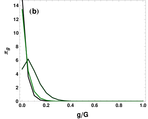
where the only exception is $g=0$ with its $n_{0}=1$. Exemplary probability distributions $\Pi_{g}$ for MERW and GRW are shown in Fig. 2.

Now, as this result depends on $\theta$ and the solutions for $\lambda$ depend on whether $r<2k$, Eq. (21), $r=2k$, Eq. (22), or $r>2k$, Eq. (27), this means that we can get different distributions for different choices of $r$. For $r<2k$, parameter $\theta\approx\frac{\pi}{G+\delta}$ and the distribution remains a sine square; for $r=2k$, $\theta=\frac{\pi/2}{G+1}$ and the distribution becomes a cosine square; for $r>2k$, $\theta=i\ \,\mathrm{arctanh}\ x$ [where $x$ is given in (28) and $i$ is the imaginary unit], thus we obtain a hyperbolic sine. Figure 3 illustrates these cases. An interactive demonstration showing these results as well as finite-size effects is available online [17].

References

- [1] A. Einstein, Ann. Phys. (Leipzig) 17, 549 (1905); 19, 371 (1906).
- [2] M. Smoluchowski, Ann. Phys. (Leipzig) 21, 756 (1906).
- [3] G. Polya, Math. Ann. 84, 149 (1921).
- [4] Z. Burda, J. Duda, J.M. Luck, and B. Waclaw, Phys. Rev. Lett. 102, 160602 (2009).
- [5] Z. Burda, J. Duda, J.M. Luck, and B. Waclaw, Acta Phys. Pol. B 41, 949 (2010).
- [6] L. Demetrius, V.M. Gundlach and G. Ochs, Theor. Popul. Biol. 65, 211 (2004).
- [7] L. Demetrius, T. Manke, Physica A 346, 682 (2005).
- [8] J.H. Hetherington, Phys. Rev. A 30, 2713 (1984).
- [9] V. Zlatic, A. Gabrielli, G. Caldarelli, Phys. Rev E 82, 066109 (2010).
- [10] J.-C. Delvenne, and A.-S. Libert, Phys. Rev. E 83, 046117 (2011).
- [11] R. Sinatra, J. Gomez-Gardenes, R. Lambiotte, Phys. Rev. 83, 030103 (2011).
- [12] C. Monthus, T. Garel, J. Phys. A - Math. Gen. 44, 085001 (2011);
- [13] K. Anand, G. Bianconi, S. Severini, Phys. Rev. E 83, 036109 (2011).
- [14]
B. Waclaw, Generic Random Walk and Maximal Entropy Random Walk,
Wolfram Demonstration Project,
http://demonstrations.wolfram.com/GenericRandomWalkAndMaximalEntropyRandomWalk/. - [15] W.M.X. Zimmer and G.M. Obermair,J. Phys. A : Math. Gen. 11, 1119 (1978).
- [16] W. Parry, Trans. Amer. Math. Soc. 112, 55 (1964).
- [17] J.K. Ochab, Stationary states of Maximal Entropy Random Walk and Generic Random Walk on Cayley trees, Wolfram Demonstration Project, http://demonstrations.wolfram.com.
- [18] J.K. Ochab, Dynamics of Maximal Entropy Random Walk and Generic Random Walk on Cayley trees, Wolfram Demonstration Project, http://demonstrations.wolfram.com.
- [19] S. Fortunato, Physics Reports 486, 75-174 (2010).