Lawrence-Krammer-Bigelow representations and dual Garside length of braids
Abstract.
We show that the span of the variable in the Lawrence-Krammer-Bigelow representation matrix of a braid is equal to the twice of the dual Garside length of the braid, as was conjectured by Krammer. Our proof is close in spirit to Bigelow’s geometric approach. The key observation is that the dual Garside length of a braid can be read off a certain labeling of its curve diagram.
Key words and phrases:
Lawrence-Krammer-Bigelow representation, Braid group, curve diagram, dual Garside length2010 Mathematics Subject Classification
Primary 20F36, Secondary 20F10,57M071. Introduction
The question whether the braid group is linear or not was a long standing problem. At the end of the 20th century, the problem was solved affirmatively by Krammer [Kra2] and Bigelow [Big] independently. They showed that a certain linear representation of the braid group first constructed by Lawrence [Law] and now called the Lawrence-Krammer-Bigelow representation (LKB representation, for short) is faithful. Interestingly, the two proofs of the faithfulness of the LKB representations are completely different: Bigelow’s proof is geometric whereas Krammer’s proof is algebraic.
Our main result is (Theorem 1.1) that the span of the variable in the image of the LKB representation of a braid is equal to twice the dual Garside length of , as conjectured by Krammer in [Kra1]. This is an analogue of Krammer’s theorem [Kra2] that the span of the variable in the image of the LKB representation is equal to the classical Garside length. It is remarkable that, despite the analogy with Krammer’s result, our proof is rather based on Bigelow’s techniques.
One of our main tools is a labeling of curve diagrams of braids called the wall crossing labeling. In Theorem 3.3, we will prove that the wall crossing labeling tells us the dual Garside length of braids. On the other hand, in Lemma 4.1 we will observe that the wall crossing labeling is also related to the variable in the noodle-fork pairing, a homological intersection pairing appearing in the LKB representation. Thus wall crossing labelings of curve diagrams serve as a bridge connecting two seemingly unrelated objects, namely the LKB representation and the dual Garside structure.
In order to state our main Theorem, we set up some notation. In this paper we denote the LKB representation by
The matrix representative depends on the choice of the basis, and there are variations of the matrices of the LKB representation: all matrices given in the three papers [Big],[Kra1],[Kra2] are different!
In this paper we use Bigelow’s expression of the matrices given in [Big, Theorem 4.1], with the correction of a sign error from [Big2]. This expression has geometric origin, and is essentially the same as the matrices in [Kra1], except that the variable of [Kra1] corresponds to of [Big].
Let us take the basis of , defined by the standard forks – see Section 2 for details. Using this basis, the matrix representative of the LKB representative is given as follows.
The image is a -matrix whose entries are in . For a Laurent polynomial , let and be the maximal and the minimal degree of the variable , respectively. For a matrix we define
We denote the supremum, the infimum and the length function of a braid for the dual Garside structure by , , and , respectively – see Section 2.1 for precise definitions.
The main result in this paper is the following, which was already conjectured by Krammer in [Kra1].
Theorem 1.1 (Variable in the LKB representation and the dual Garside length).
For ,
- (1)
.
- (2)
.
- (3)
.
Acknowledgement
The first author was supported by the JSPS Institutional Program for Young Researcher Overseas Visits.
2. Preliminaries
First of all we set up our notation and conventions. Let be the unit disc in the complex plane and be the -punctured disc, where each puncture is put on the real line so that holds. The braid group is identified with the mapping class group of .
Thoroughout this paper, we adopt the following conventions. Braids acts on the left. A positive standard generator is identified with the left-handed, that is, the clockwise half Dehn-twist which interchanges the punctures and . Also, when calculating winding numbers, the positive direction of winding is taken as the clockwise direction. This convention is the opposite to Bigelow’s.
2.1. The dual Garside length
First we review the definition of the supremum, the infimum and the length functions of the dual Garside structure. We do not need detailed Garside theory such as normal forms or algorithms. We only need a length formula, Proposition 2.1 below.
Recall that the braid group is presented as
The elements of the generating set are called Artin generators or Garside generators.
In the dual Garside structure, we use a slightly different generating set which contains as a subset. For , let be the braid
The generating set was introduced in [BKL], and its elements are called the dual Garside generators, or band generators, or Birman-Ko-Lee generators. In our conventions, the braid is represented by the left-handed half Dehn-twist along an arc connecting and in the lower-half of the disc .
A dual-positive braid is a braid which is written by a product of positive dual Garside generator . The set of dual-positive braids is denoted by . The dual Garside element is a braid given by
Let be the subword partial ordering with respect to the dual Garside generating set : if and only if . For a given braid , the supremum and the infimum is defined by
and
respectively. A dual-simple element is a dual-positive braid which satisfies . The set of dual-simple element is denoted by . The Garside length is the length function with respect to the generating set .
The next formula relates the supremum, infimum and the length.
Proposition 2.1 (Dual Garside length).
For a braid we have the following equality
See [BKL] for proof.
2.2. The Lawrence-Krammer-Bigelow representation of the braid groups
We review a definition of the Lawrence-Krammer-Bigelow representation. Our description of the LKB representation is homological and mainly follows Bigelow, but it is slightly modified so as to agree with our conventions. For details, see [Big].
Let be the configuration space of two unordered points of . We take base points and in so that lies on the right side of – see Figure 1. We take as a base point of .
Let be the free abelian group of rank two generated and , and define a homomorphism as follows: let a loop representing an element . We define the number as the sum of the winding numbers along each puncture :
We define the number as twice the winding number of the path (i.e. as twice the relative winding number of the points):
Now we define . (Here we add the minus signs since we adapted the convention that the positive winding direction is the clockwise direction.)
Let be the covering of associated to . Fix the lift of the base point . By abuse of notation, we use the same symbol to represent the base point both in and . Then and are regarded as deck translations and the second homology group is a -module.
Let be the -shaped graph shown in Figure 1, having one distinguished external vertex , two other external vertices and , and one internal vertex . We orient the edges of as shown in Figure 1.

A fork is an embedded image of into such that:
- •
All points of are mapped to the interior of .
- •
The distinguished vertex is mapped to the base point .
- •
The other two external vertices and are mapped to two different puncture points.
- •
The edge and the arc are both mapped smoothly.
The image of the edge is called the handle of . The image of , regarded as a single oriented arc, is called the tine, denoted . The image of is called the branch point of .
A parallel fork is a fork as depicted by a dotted line in Figure 1: is parallel to and the distinguished vertex is mapped to .
A noodle is an oriented smooth embedded arc which begins at and ends at .
Let be the handles of the forks and of its parallel , respectively. Let be the lift of the path taken so that .
Consider the surface in . Let be the component of which contains the point . The surface in defines an element of . By abuse of notation, we will use the same symbol to represent the 2nd homology class defined by the surface . In a similar way, a noodle defines a surface which defines an element of . Again, by abuse of notation we denote the homology class by .
For , let us take a fork as shown in Figure 2. These forks are called standard forks. We call a standard fork of the form a straight fork. Similarly, let be the noodle which encloses the -th puncture point as shown in Figure 2. We call such a noodle a standard noodle. Bigelow showed that is a free -module and is a basis of . From now on, by using this basis we always identify with .

The braid group acts on the covering so that it commutes with the deck translations and . Hence we get a representation . The exact matrices are given in the Introduction. This is the Lawrence-Krammer-Bigelow (LKB) representation.
Remark 2.2.
As shown in [PP], the standard forks do not form a basis of the -module . Thus in the above description it was important to use real coefficients, even if the matrix coefficients actually all lie in .
2.3. Noodle-fork pairings
The Noodle-Fork pairing is a homology intersection pairing . As Bigelow showed in his so-called Basic Lemma ([Big, Lemma 2.3]), the pairing is calculated as follows.
Let be the intersection points of with , and let be the intersection of with which corresponds to .
Observe that a pair of intersection points corresponds to an intersection point of the surfaces and . Hence it contributes to the total intersection pairing of and as a monomial where denotes the sign of the intersection at .
The monomial is computed as follows. First we define by
Take three paths and in as follows:
- •
is a path from to the branch point of along the handle of .
- •
is a path from the branch point to along the tine .
- •
is a path from to along the noodle . Here if and if . In other words, goes along starting from , choosing the direction so as to avoid .
Similarly, we take three paths and by
- •
is a path from to the branch point of along the handle of .
- •
is a path from the branch point to along the tine .
- •
is a path from to along the noodle . Here if and if .
Now the concatenation of the three paths defines a loop in . The monomial is given by . The sign of the intersection is given by
where (respectively ) is the sign of the intersection of and (respectively ) at (respectively ).
In summary, the noodle-fork pairing is given by the following sum, where we recall that denotes the number of intersections of with :
By direct computations we observe the following, which will play an important role in the proof of main theorems.
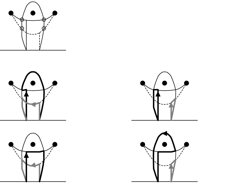
Lemma 2.3.
Let be a standard noodle and let be a standard fork. Then
Proof.
Here we give the calculation of the paring , for the most complicated case, the other cases are treated similarly. Let and be a standard fork and noodle and assume that . Then and intersect at two points, and hence the two surfaces and intersects at four points. Now and are calculated as shown in Figure 3. The paths and are depicted by a black and gray line, respectively. Thus, we conclude . ∎
3. The wall crossing labeling of curve diagrams
In this section we introduce the wall crossing labeling on curve diagrams and show that this labeling reflects the dual Garside length of braids. This result is interesting in its own right.
3.1. Curve diagrams
Let be the diagram in consisting of the real line segment between the point (the leftmost point of ) and (the rightmost puncture). Similarly, let be the diagram in consisting of the real line segment between (the leftmost puncture) and (the rightmost puncture). Both line segments and are oriented from left to right. Let be a vertical line segment in , oriented upwards, which connects the puncture and the boundary of in the upper half-disk – see Figure 4. The lines are called the walls, and their union is denoted .
 and
and
For , the total curve diagram and the curve diagram of is the image of the diagrams and , respectively, under a diffeomorphism representing which satisfies the following conditions.
- (1)
The number of intersections of with the walls is as small as possible within the diffeotopy class of .
- (2)
Near the puncture points, the image coincides with the real line.
We denote the curve diagram of by and the total curve diagram by . See the right side of Figure 4 for an example.
To introduce the wall-crossing labeling and make the correspondence between fork and curve diagram explicit, we use a modified version of the curve diagrams. For each puncture other than , we take a small disc neighborhood of , say , and let . Around each puncture , we modify the curve diagram as shown in Figure 5. We denote the resulting (total) curve diagram by , and call it the (total) modified curve diagram. The right side of Figure 5 shows the total modified curve diagram of .

Take a smooth parametrization of , viewed as an image of the function . Then we define the wall crossing labeling as follows.
Definition 3.1.
Let be the set of intersection points . For each connected component of , we assign the algebraic intersection number of and the arc , where is taken so that . We call this integer-valued labeling the wall crossing labeling.
An arc segment of the curve diagram (or the total curve diagram ) is a component of (or of , respectively). Since and coincide except on , an arc segment is identified with the subarc of . Using this correspondence, we assign the wall crossing labeling for each arc segment of the curve diagram – see Figure 6.
Definition 3.2.
For a braid , we define and as the largest and the smallest wall crossing number labelings occurring in the curve diagram .
Notice that in Definition 3.2 we used the largest and smallest labels only of the curve diagram , not the total curve digram . However, in order to determine the wall crossing labelings we need to consider the total curve diagram.
We now show that the dual Garside (Birman-Ko-Lee) length of a braid can be read off the wall crossing labeling of its curve diagram.
Theorem 3.3.
For a braid we have the following equalities:
- (1)
.
- (2)
.
- (3)
.
Example 3.4.
Let us consider the braid – see Figure 6. Any word representing this braid with letters belonging to has at least two negative letters, so . Similarly, any word representing using these letters has at least two positive letters, so . (Indeed, the dual normal form of is .)
Proof of Theorem 3.3.
First of all, we show that for a dual-positive braid the equality holds.
To treat the dual Garside structure, we temporarily isotope our curve diagram and walls so that the all punctures sit on the circle and walls are disjoint from the subdisc as shown on the left side of Figure 7. This isotopy does not affect the wall crossing labelings, since the wall crossing labeling is defined by using algebraic intersection of arcs and walls.
As shown in [BKL], the set of dual-simple braids is in bijection with the set of disjoint collections of convex polygons in whose vertices are punctures. This bijection is given as follows: to any such collection of polygons we can associate a dance of the puncture points, moving each puncture which belongs to some polygon in the clockwise direction along the boundary of , to the position of the adjacent vertex. In this way, each dual-simple element can be represented by some disjoint convex polygons in – see Figure 7.
We remark that polygons may be degenerate, having only two vertices; in the associated braids, the two corresponding punctures are interchanged by a clockwise half Dehn-twist.

Given a curve diagram , equipped with the wall crossing labeling, and given a collection of disjoint polygons with vertices in the punctures representing some dual-simple braid , let us describe in detail how to obtain the curve diagram and its wall crossing labeling. Consider the disjoint collection of annuli in as follows (see Figure 8):
- (1)
The outer and inner boundary component of are both homotopic in to the boundary of a regular neighborhood of .
- (2)
The boundary components of are in reduced relative position (no bigons) with respect to the walls and also with respect to the curve diagram .
- (3)
Let us denote the components of containing the polygon by . Note that the intersection of with is simply a spiral, and that the labels on this spiral interpolate linearly between the labels on the outer and inner boundary component.
Now the -action on is simple to describe: on , the diagram and its labeling is unchanged. On the diagram is turned one notch in the clockwise sense, and all labels are increased by one. On the annuli, we have some twisting, but the labels still just interpolate - see Figure 8.

The action of a negative dual-simple braid is similar, the only difference being that the twisting is in the counterclockwise direction and labels are decreased by one.
From the above description for a dual-positive braid and a dual-simple element , we have the inequality . This implies the inequality
The converse inequality is now implied by the following lemma:
Lemma 3.5.
The dual-positive braid can be written as the product of positive dual-simple braids.
Proof of Lemma 3.5.
From the above description of the action of a dual-positive braid, we see that , as no negative labels can ever be created from non-negative ones.
In order to prove the lemma, we distinguish two cases. Firstly, if , then no arc of the modified curve diagram crosses a wall. This implies that is a power of , more precisely, , and the lemma is true.
Secondly, if , then we proceed inductively. We shall construct a negative dual-simple braid such that and .
Consider the arc segments having the maximal wall crossing labeling. Each such segment connects two walls. Let be the pairs of walls which are connected by some maximal labeled arcs. Let be the minimal (with respect to inclusion) collection of convex polygons which contains all straight lines connecting and for . Let be the inverse of the dual-simple braid that corresponds to . Garside theoretically speaking, .
According to our description above of the -action on the curve diagram , the action of decreases all the maximal wall crossing labelings by one, so .
On the other hand, we claim that , i.e., contrary to the largest label, the smallest label does not decrease during the -action.
Let us prove this claim. First we observe that, roughly speaking, minimally labeled arcs are S-shaped, whereas maximally labeled arcs are S -shaped. More precisely, when both endpoints of a minimally labeled arc lie in the interior of walls, then the initial and terminal segment of the arc lie on the counterclockwise sides of the wall, whereas maximally labeled arcs begin and terminate on clockwise sides of the respective walls (see Figure 9(a)).
Now, in order to prove the claim, we have to rule out the existence of minimally labeled arcs (i.e. arcs labeled ) which, under the -action, give rise to arcs with an even smaller label.
First we observe that a minimally labeled arc cannot intersect the interior of any of the polygons of . Indeed, assume that an arc segment enters into the interior of one of these polygons, say . Let us assume in addition that both endpoints of lie in the interior of walls, not in punctures. Then cuts into two components, and thus separates the vertex punctures of into two families (drawn white and black in Figure 9(a)). Now we observe that no maximally labeled arc can connect a wall belonging to a black puncture to a wall belonging to a white puncture. But, by construction of , that means that the white and black punctures do not belong to the same polygon , which is a contradiction.
 forbidden
allowed:
forbidden
Example of a
max. labeled arc
(a)
(b)
(c)
forbidden
allowed:
forbidden
Example of a
max. labeled arc
(a)
(b)
(c)
Similarly, when a minimally labeled arc intersects the interior of but has one or both endpoints in punctures, then the same argument applies, we only have to decide in which color to paint a puncture at the extremity of . The choice which works is to group such a puncture with the following punctures in the clockwise direction – see Figure 9(a).
Finally, we have to consider a minimally labeled arc segment which ends in a vertex of without intersecting the interior of . Here we have to distinguish two cases. If an extremal segment of lies on the counterclockwise side of the wall corresponding to its terminal puncture, as in Figure 9(b), then there is nothing to worry about since the -action does not decrease its Wcr-label. If, on the other hand, a terminal segment of lies on the clockwise side of the wall corresponding to its terminal puncture, as in Figure 9(c), then this wall cannot be connected to a wall of any of the other punctures of by a maximally labeled arc. Again, this contradicts the construction of .
In summary, no minimally labeled arc can generate an even smaller label under the -action. This proves the claim, and thus Lemma 3.5. ∎
To summarize, we have now proved that for a dual-positive braid , the following equality holds:
For a dual-positive braid , so by Proposition 2.1 we conclude that
In a similar way, we prove the equality for any dual-negative braid .
In order to prove the same results for arbitrary braids, we recall that the dual Garside element acts as the clockwise –rotation of the -gon with vertices in all punctures. Thus the curve diagram is obtained from simply by a –rotation, and the wall crossing labeling on each arc segment of is obtained from the label of the corresponding arc of by adding one. On the other hand, by definition of and , left multiplication by increases both and by one. Therefore for a general braid , we get an equality
A similar calculation also yields
for a general braid . Finally, Proposition 2.1 implies the third equality claimed in Theorem 3.3. This completes the proof of Theorem 3.3. ∎
Remark 3.6.
In [W] the second author defined another labeling on the curve diagram called the winding number labeling, and proved the similar formula for the winding number labeling and the usual Garside length ([W, Theorem 2.1]). The proof of Theorem 3.3 given here is a direct generalization of the proof of [W, Theorem 2.1].
4. Noodle-fork pairing and wall crossing labeling
In this section we make the observation (in Lemma 4.1) that the wall crossing labeling reflects the exponents of the variable in the noodle-fork pairing.
We need some technical preparation for this. We first show that for any straight fork , and for any braid , the tine can in a natural way be equipped with the wall crossing labeling. For this, we will have to relate curve diagrams and forks.
Let us consider the part of the curve diagram that is the image of the line segment between the -th and -st punctures. We identify this part of the curve diagram with , the image of the tine of the straight fork . Moreover, up to moving the footpoint from to , part of the modified curve diagram can naturally be regarded as the handle of , as shown in Figure 10. This identification also induces the desired wall crossing labelling on each arc segment of .

Let be a standard noodle, and let be a straight fork with tine . Consider the image of a straight fork . From now on, we always assume that is isotoped so that it intersects minimally. For an intersection point , we denote the wall crossing labeling of the arc segment of containing by . We recall that the union of the walls is denoted . We also recall that the intersection pairing of and is where the sum ranges over all pairs of intersection points .
Lemma 4.1.
Let be a straight fork and let be a standard noodle. Let be the set of intersection points of and . Then , the exponent of at the intersection point is given as follows.
Proof.
Recall that is defined as the sum of the winding numbers of the paths and around each puncture:

For a closed loop in , the winding number around the puncture
is equal to the algebraic intersection number of and . Thus, the fork part of the path , namely the subarc , contributes to the total winding number by . Finally, we observe that the rest of the loop (the noodle part of the path ) contributes to the total winding number by (respectively ) if and belongs to the same (respectively to different) components of – see Figure 11. This completes the proof. ∎
Remark 4.2.
For the winding number labeling introduced in [W], and for , the exponent of at the intersection , one can get a similar formula by similar arguments.
Thus, schematically speaking, we have the following correspondence among three objects in braid groups:
| LKB representation | Curve diagram | Garside structure |
|---|---|---|
| Variable | Winding number labeling | Usual Garside structure |
| Variable | Wall crossing labeling | Dual Garside structure |
5. The dual Garside length formula
In this section we prove Theorem 1.1. For monomials and we define the lexicographical ordering by
The next lemma is the crucial result in Bigelow’s proof of faithfulness.
Lemma 5.1.
[Big, Bigelow’s Key Lemma 3.2 and Claim 3.4] Assume that a noodle and a fork have the minimal geometric intersection. Then all intersection points of with which attain the -maximal monomial in have the same sign .
Roughly speaking, Lemma 5.1 states that the -maximal contributions to do not cancel.
Lemma 5.2.
Let be a braid. Let be a straight fork such that contains an arc segment having the largest wall crossing labeling . Then there exists a standard noodle such that
Proof.
Throughout proof, we assume that intersects each standard noodle minimally. It is sufficient to show that there is a standard noodle and an intersection point such that and such that the two points and lie in the same component of : by Lemma 4.1, the intersection point contributes to the pairing by for some , and then Lemma 5.1 completes the proof.
 (a)
(b)
(c)
(d)
(a)
(b)
(c)
(d)
Let be an arc segment of whose wall crossing labeling is . Take a standard noodle which intersects in a point . Assume that and lie on the two different components of . If does not fall into the puncture , then we can find another intersection point of with that lies on the same component of as (Figure 12 (a)) and the proof is complete. Assume that falls into the puncture . Then must pass under the adjacent puncture because otherwise we either find another arc segment having strictly larger wall crossing labeling (Figure 12 (b)) or contradict the hypothesis that and have the minimal intersection (Figure 12 (c)). Then the standard noodle and have an intersection with the desired property (Figure 12(d)). ∎
Proof of Theorem 1.1.
For a braid , let us take a straight fork and a standard noodle as in Lemma 5.2. Thus we have . Let us write the fork as the linear combination of the standard forks
Since is a straight fork, is an entry of the matrix . Now we have an equality
Since in Lemma 2.3 we observed that
we conclude
where the second inequality follows from Lemma 5.2 and the last equality from Theorem 3.3. Thus, we get an inequality
On the other hand, for each dual-simple element
holds. Hence we get the converse inequality
We conclude that
The proof of (2) is similar, and (3) follows from Proposition 2.1. ∎
References
- [Big] S. Bigelow, Braid groups are linear, J. Amer. Math. Soc. 14, (2000), 471–486.
- [Big2] S. Bigelow, The Lawrence-Krammer representation, Topology and geometry of manifolds (Athens, GA, 2001), 51–68, Proc. Sympos. Pure Math., 71, Amer. Math. Soc., Providence, RI, 2003.
- [BKL] J. Birman, K.H. Ko, and S.J. Lee, A new approach to the word problem in the braid groups, Adv. Math. 139 (1998), 322–353.
- [Kra1] D. Krammer, The braid group is linear, Invent. Math. 142, (2000), 451–486.
- [Kra2] D. Krammer, Braid groups are linear, Ann. Math. 155, (2002), 131–156.
- [Law] R. Lawrence, Homological representations of the Hecke algebra, Comm. Math. Phys. 135, (1990), 141–191.
- [PP] L. Paoluzzi, L. Paris, A note on the Lawrence-Krammer-Bigelow representation, Algebr. Geom. Topol. 2 (2002), 499–518
- [W] B. Wiest, How to read the length from its curve diagram, Groups Geom. Dyn. 5, (2011), 673–681.