On The Convergence of Gradient Descent for Finding the Riemannian Center of MassThanks: The authors were supported in part by grants NSF CAREER # 0447739, NSF CNS # 0834470, ONR # N00014-05-10836, and ONR # N00014-09-1-0084
Abstract.
We study the problem of finding the global Riemannian center of mass of a set of data points on a Riemannian manifold. Specifically, we investigate the convergence of constant step-size gradient descent algorithms for solving this problem. The challenge is that often the underlying cost function is neither globally differentiable nor convex, and despite this one would like to have guaranteed convergence to the global minimizer. After some necessary preparations we state a conjecture which we argue is the best convergence condition (in a specific described sense) that one can hope for. The conjecture specifies conditions on the spread of the data points, step-size range, and the location of the initial condition (i.e., the region of convergence) of the algorithm. These conditions depend on the topology and the curvature of the manifold and can be conveniently described in terms of the injectivity radius and the sectional curvatures of the manifold. For manifolds of constant nonnegative curvature (e.g., the sphere and the rotation group in ) we show that the conjecture holds true (we do this by proving and using a comparison theorem which seems to be of a different nature from the standard comparison theorems in Riemannian geometry). For manifolds of arbitrary curvature we prove convergence results which are weaker than the conjectured one (but still superior over the available results). We also briefly study the effect of the configuration of the data points on the speed of convergence.
Key words and phrases:
Riemannian center of mass, Fréchet mean, Riemannian mean, Riemannian average, gradient descent, spherical geometry, spherical trigonometry, comparison theorems, gradient descent, convergence analysis, global convergence2010 Mathematics Subject Classification
Primary 53C20, 90C25, 90C26; Secondary 62H11, 68U05, 92C551. Introduction and Outline
The (global) Riemannian center of mass (a.k.a. Riemannian mean or average or Fréchet mean)11 1 Throughout this paper we are mainly interested in the “global” Riemannian center of mass, hence in reference to it very often we drop the term “global” and simply use “Riemannian center of mass,” etc. If need arises we explicitly use the term “local” in reference to a center which is not global (see Definition 2.5). of a set data points in a Riemannian manifold is defined as a point which minimizes the sum of squares of geodesic distances to the data points. This notion and its variants have a long history with several applications in pure mathematics (see e.g., [6], [17], [19], [22] and also [3] for a brief history and some new results). More recently, statistical analysis on Riemannian manifolds and, in particular, the Riemannian center of mass have found applications in many applied fields. These include fields such as computer vision (see e.g., [36] and [35]), statistical analysis of shapes (see e.g., [21], [25], [8], [15], and [7]), medical imaging (see e.g., [14] and [30]), and sensor networks (see e.g., [34] and [33]), and many other general data analysis applications (see e.g., [23], [2], [9], and [29]). In these applied settings one often needs to numerically locate or compute the Riemannian center of mass of a set of data points lying on a Riemannian manifold, and the so-called (intrinsic) gradient descent algorithm has been a popular choice for this purpose. The constant step-size version of the gradient descent for finding the Riemannian center of mass is the easiest one to implement, and hence is the most popular one.
The main challenge in analyzing as well as working with the constant step-size gradient descent algorithm for finding the Riemannian center of mass is the fact that the underlying cost function is usually neither globally differentiable 22 2 For us global differentiability means differentiability everywhere on the manifold; however, we use the term “global” to remind ourselves that our functions of interest (e.g., the Riemannian distance from a point) lose differentiability at far away distances. nor globally convex on the manifold.33 3 In fact, it is well known that on a compact Riemannian manifold the only globally continuous convex functions are constant functions (see Theorem 2.2 and [39]). More specifically, the cost function is not differentiable at any cut point of the data points. Moreover, as it can be shown by simple examples, the cost function can have local minimizers, which are not of interest and should be avoided. Nevertheless, we expect and hope that if the algorithm is initialized close enough to the (unknown) global Riemannian center of mass and the step-size is small enough, then the algorithm should converge to the center. One would like to have the step-size small enough such that the cost is reduced at each step and at the same time the iterates do not leave a neighborhood around in which is the only zero of the gradient of the cost function (recall that a gradient descent algorithm, at best, can only locate a zero of the gradient vector field of the cost function). On the other hand, one would like to have large enough step-size so that the convergence is fast. The interplay between these three constraints is important in determining the conditions guaranteeing convergence as well as the speed of convergence.
The goal of this paper is to give accurate conditions that guarantee convergence of the constant step-size gradient algorithm to the global Riemannian center of mass of a set of data points. In Section 2, we first briefly give the necessary backgrounds on the Riemannian center of mass and the gradient descent algorithm for finding it, these include the notions of convex functions and sets in Subsection 2.1.2, differentiability and convexity properties of the Riemannian distance function and bounds on its Hessian in Subsection 2.1.3, Riemannian center of mass and its properties in Subsection 2.1.4, a general convergence theorem for gradient descent in Subsection 2.1.5, and a convergence theorem estimating the speed of convergence and the best step-size in Subsection 2.1.6. Following that, in Subsection 2.2, we state Conjecture 2.15 in which we specify the best “condition for convergence” one can hope for (in a sense to be described). Specifically, we specify a bound on the radius of any ball around the data points in which the algorithm can be initialized together with an interval of allowable step-size so that the algorithm converges to the global center of mass . The significant point is that for convergence the radius of the ball does not need to be any smaller than what ensures existence and uniqueness of the center. Moreover, the step-size can be chosen equal to the best (in a specific described sense) step-size under the extra assumption that the iterates stay in that ball; 44 4 This step-size, in general, depends on an upper bound on the sectional curvatures of the manifold and the radius of the mentioned ball. However, interestingly, for a manifold of non-negative curvature it is simply (see Conjecture 2.15 and Remark 2.16). and it is conjectured that, indeed, the iterates stay in the ball. 55 5 The main challenge in proving this conjecture is to prove that the iterates stay in the ball containing the data points. Knowing the conjecture helps us to compare and evaluate the existing results mentioned in Subsection 2.3 as well as the results derived in this paper. In Section 3 (Theorem 3.6), we prove Conjecture 2.15 for the case of manifolds of constant nonnegative curvature. In our developments in this section, we first prove comparison Theorem 3.1 in Subsection 3.1. This comparison result (which differs from standard comparison theorems in some aspects) most likely has been known among geometers, but we could find neither its statement or a proof for it in the literature. In Subsection 3.2 we make sense of an intuitive notion of Riemannian affine convex combination of a set of data points in a manifold of nonnegative constant curvature and we explore its relation to the convex hull of the data points. These prepare us to prove the main theorem of the section, Theorem 3.6, in Subsection 3.3. Although limited in scope, this result covers some very important manifolds of practical interest: the unit sphere in , the group of rotations in , and the real projective space in . In Section 4, for manifolds of arbitrary (i.e., non-constant) curvature, we derive two classes of sub-optimal convergence conditions (in comparison with Conjecture 2.15): In Subsection 4.1 we give a result (Theorem 4.1) in which convergence is guaranteed at the expense of smaller spread of data points, whereas in Subsection 4.2 (Theorem 4.2) the allowable step-size is compromised to guarantee convergence. Finally, in Section 5, we qualitatively identify data configurations for which the convergence is very fast or very slow. We conclude the paper in Section 6 by giving some remarks about further research.
2. Preliminaries, a conjecture, and prior work
2.1. Preliminaries on the Riemannian Center of Mass and the Gradient Descent Algorithm
2.1.1. Notations
Let be an -dimensional complete66 6 Our results are local in nature, but they hold in relatively large regions that are determined explicitly. Therefore, completeness of the manifold is not necessary and our results could be easily adapted to e.g., non-singular regions of a singular manifold. However, for this purpose the statements of our results could become rather cumbersome. Riemannian manifold with distance function .77 7 In our definitions relating to Riemannian manifolds we mainly follow [32]. We denote the tangent space at by and by and we mean the Riemannian structure and the corresponding norm, respectively (dependence on the base point is implicit and clear from the context). By a function in a subset of we mean a continuous function which is order continuously differentiable in the subset as commonly understood in differential geometry. For a function , denotes its gradient vector field with respect to . We assume that the sectional curvatures of are bounded from above and below by and , respectively. The exponential map of at is denoted by and its inverse (wherever defined) is denoted by . The injectivity radius of is denoted by . An open ball with center and radius is denoted by and its closure by .
2.1.2. Convex functions and sets in Riemannian manifolds
Convexity plays an important rule in our developments and we have the following definition:
Definition 2.1.
Let be an open subset of such that every two points in can be connected by at least one geodesic of such that this geodesic lies entirely in . Assume that is a continuous function. Then is called (strictly) convex if the composition is (strictly) convex for any geodesic . We say that is globally (strictly) convex if it is (strictly) convex in .
If is in , then convexity (strict convexity) of is equivalent to (), where is any geodesic in .
An insightful fact is the following [39]:
Theorem 2.2.
The only globally convex function in a compact Riemannian manifold is a constant function.
It is more convenient to limit ourselves to strongly convex subsets of because they are quite similar to standard convex sets in :
Definition 2.3.
A set is called strongly convex if any two points in can be connected by a unique minimizing geodesic in and the geodesic segment lies entirely in .
Define
| (2.1) |
with the convention that for . An open ball with is strongly convex in ; the same holds for any closed ball if (see e.g., [32, p. 404] and [11, pp. 168-9]). In fact, with is even more similar to a convex set in Euclidean space: for any the minimal geodesic between from to is the only geodesic connecting them which lies entirely in .
2.1.3. Differentiability and convexity properties of the distance function and estimates on its Hessian
Now, we briefly give some facts about the Riemannian distance function which will be used throughout the paper. Let . The function is continuous for every . However, it is differentiable (in fact ) in , where is the cut locus of (see e.g., [32, pp. 108-110]). We recall the notion of cut locus: Let be the largest domain containing the origin of in which is a diffeomorphism, and let be the boundary of . Then is called the cut locus of and one has (see e.g., [11, pp. 117-118] or [32, p. 104]). The distance between and is called the injectivity radius of denoted by , and by definition . It is well known that has measure zero in . On the unit sphere the cut locus of every point is its antipode. In a general manifold the differentiability property of at is similar to the case where equipped with the standard Euclidean metric; in particular, is a function in . However, the behavior at far away points (e.g., the cut locus) is of substantially different nature and depends on the topology and curvature of (recall that in Euclidean space the cut locus of every point is empty).
Next, we recall some useful estimates about the Hessian of the Riemannian distance function. We adopt the following definitions:
| (2.2) |
and
| (2.3) |
Assume that is such that .88 8 Instead of this condition, it is often more convenient to require , which is a more conservative yet global version of the condition. Furthermore, assume that with is a unit speed geodesic making, at , an angle with the minimal geodesic from to . It can be proved that (see e.g., [32, pp. 152-154])
| (2.4) |
where is defined in (2.2). Based on the above one can verify that
| (2.5) |
and more generally that
| (2.6) |
Notice that the above confirms the intuition that the differentiability behavior of at is the same in and in . We will use these two relations very often; in doing so it is useful to have in mind that and , respectively, are decreasing and increasing in .
Remark 2.4.
We emphasize that the requirement is essential and cannot be compromised, as at a cut point the distance function becomes non-differentiable. Although in the left hand side of the above bounds only appears explicitly both the curvature and topology of determine the convexity properties of the distance function. Notice that gives (some) information about the Riemannian curvature tensor of and (or ) gives (some) information about the topology of . For example, and the unit circle both have zero sectional curvature, while and the injectivity radius of is infinity. Now obviously in is globally convex, while in it is not (as seen directly or as a consequence of Theorem 2.2). The interesting fact is that has positive definite Hessian in , where is the antipodal point of . At , is not differentiable. This non-differentiability is so severe that in spite of the positivity of its Hessian at all other points is far from a globally convex function on . As an example of a less severe non-differentiability notice that in is also non-differentiable at , yet this does not affect its convexity.
2.1.4. Riemannian center of mass
We start by the following definition:
Definition 2.5.
The (global) the Riemannian center of mass or mean (a.k.a. Fréchet mean) of the data set with respect to weights () is defined as the minimizer(s) of
| (2.7) |
in . We denote the center by . We call a local minimizer of (which is not global) a local center of mass of the data set with respect to the weights.99 9 A local minimizer of in is sometimes called a Karcher mean, although this definition bears little relation with the way Grove and Karcher [17] or Karcher [19] originally defined what they called the Riemannian center of mass (see also [3] for more details). Given with small enough those authors defined the center of mass as a zero of in or alternatively as a local minimizer of in (Notice that given that is not differentiable at the cut locus of each data point it is not a-priori clear that, in general, a local minimizer of in should coincide with a zero of , although there are some evidence in the literature that this situation might not happen, see e.g,. [18], [10]). Overall, there is no consensus among authors about the terminology and we find it more convenient to use “local” and “global” Riemannian center of mass as defined here.
The reader is referred to [3] for details and other related definitions. As a convention when referring to the center of mass of some data points we usually do not refer to explicit weights unless needed. As another convention when is not specified we assume , which is the most commonly used case. Although and are also used often, in this paper our focus is limited to .1010 10 Going from to does not introduce any major technical challenge, so our analysis can be applied almost uniformly to . However, since the results for are easier to state and presumably used more often, we usually state a result for and then give the more general version for . The only exception is Theorem 4.2 for which we do not give a version. The reason is that in our analysis we require to be twice-continuously differentiable and we determine the constant step-size of the gradient algorithm in terms of the upper bounds on the eigenvalues Hessian of . As in Euclidean case, in the more general Riemannian case also one can see from (2.6) that for the Hessian of might be unbounded. It is well known that Lipschitz continuous Hessian (in particular bounded Hessian) is necessary for the convergence of a gradient descent method with constant-step size [31].
Although is a globally convex function when is a Euclidean space (or more generally an Hadamard manifold), is not globally convex for an arbitrary . In particular, the center of mass might not be unique; however, if the data points are close enough, then the center is unique. The following theorem gives sufficient conditions for existence and uniqueness of the Riemannian center of mass.
Theorem 2.6.
Let and assume with . For , if , then the Riemannian center of mass is unique and is inside . For it is the unique zero of the gradient vector field in , and moreover if no data point has weight , then is a non-degenerate critical point of (i.e., the Hessian of at is positive-definite). 1111 11 In Theorem 2.1 of [3], the condition on is stated as , but since we have finite number of data points the current version follows immediately. Also from the statement of Theorem 2.1, is the only zero of in , but from the proof of the theorem it can be seen that the vector field is inward-pointing on the boundary of and hence is the only zero in entire . In addition, the fact about non-degeneracy is not present in the statement of Theorem 2.1 of [3], however it is proved in the proof of the theorem.
For a proof see [3]. Also for see [3] and [38]. In this paper, we are mainly interested in , because the bounds we derive on the step-size of the gradient descent algorithm depend on an upper bound on the eigenvalues of the Hessian of , and for (and ) the Hessian is unbounded. We refer the reader to [38] and [5] for algorithms in the case of and .
A rather subtle issue is that according to Theorem 2.6, if , then has a unique minimizer in . Nevertheless, , the restriction of to , might not be a convex function. More accurately, if (cf. (2.1)), then is a convex function (this can be seen easily from (2.5) by noting that for ). However, if and , then might not be a convex function, as can be seen by very simple examples. While this fact does not harm implementation and convergence of a gradient descent algorithm for finding greatly, it has some serious implications on implementation and applicability of Newton’s method (see Remarks 2.14 and 2.19).
2.1.5. Gradient descent algorithm for finding the Riemannian center of mass
For later reference we derive the intrinsic gradient descent algorithm for locating the Riemannian center of mass (see [1] or [37] for introduction to optimization on Riemannian manifolds). One can check that
| (2.8) |
for any as long as it is not in the cut locus of any of the data points. In particular, if , where , then for any the above expression is well-defined in the classical sense (i.e., it is uniquely defined). Notice that the above expression is well-defined for almost every because the set at which is not differentiable has measure zero (for this set is and for it is ). As we will see this non-differentiability has severe implications on the behavior of the constant step-size gradient descent.
Algorithm 1 in Table 1 is a gradient descent algorithm for locating the Riemannian center of mass of .
| Algorithm 1: Gradient Descent for finding the Riemannian center of mass |
| (1) Consider and weights and choose . (2) if then stop, else set (2.9) where is an “appropriate” step-size and is defined in (2.8). (3) goto step 2. |
Besides practical considerations (e.g., stopping criterion), at least two important issues are left unspecified in Algorithm 1, namely, how to choose and how to choose for each . The most natural choice for is one point in , say one of the data points. Note that in practice and the exact value of might not be known.
The choice of is more complicated. The next general proposition gives a prescription for a step-size interval which ensures reducing the cost function at an iteration of a gradient descent provided one knows an upper bound on the eigenvalues of the Hessian of the cost function in a region which iterates live. The proof of this proposition follows from the second order Taylor series expansion (with remainder).
Proposition 2.7.
Let and consider an open neighborhood containing . Let be a function whose restriction to is twice-continuously differentiable and let the real number be an upper bound on the eigenvalues of the Hessian of in . There exists such that for all the curve does not leave and
| (2.10) |
For , with the convention that for , we have with equality only if is a critical point of . Moreover, when the right hand side of (2.10) is minimized for .
Notice that the fact that for the curve stays in is crucial in enabling us to use the upper bound and derive (2.10). This concept appears frequently in our analysis and it useful to have the following definition:
Definition 2.8.
Obviously, continuously staying in is stronger than staying in . However, they are equivalent under some conditions (which hold in some, but not all, of the cases we study, see Remark 2.18):
Proposition 2.9.
If is a strongly convex set and for every , then for the iterates of Algorithm 1 staying in implies (and hence is equivalent to) continuously staying in .
Proof.
Assume that and both belong to . Recall that for is a minimizing geodesic if . Therefore, by strong convexity of , for must be the only minimizing geodesic between and and must lie in entirely. ∎
As mentioned before we are only interested in constant step-size gradient descent. The following convergence result is standard for this type of algorithms when the cost is (or at least has Lipschitz gradient) and is globally convex; however, our version is adapted to which, in general, is neither globally nor convex. The assumption of the theorem that each iterate of the algorithm continuously stay in a neighborhood of , in which is is the only zero of , is a crucial enabling ingredient of the proof. In fact, our goal in Sections 3 and 4 is essentially to identify such a neighborhood (under certain conditions).
Theorem 2.10.
Let and assume that is the center of mass of , where . Let be a bounded open neighborhood of such that is in and in , the closure of . Furthermore, assume that is the only zero of the vector field in . Let be an upper bound on the eigenvalues of the Hessian of in . In Algorithm 1 choose . If starting from , each iterate of Algorithm 1 continuously stays in , then for with equality only if and converges to .
Proof.
Since by assumption for and is compact, there is a subsequence converging to a point . By Proposition 2.7 we have unless and furthermore
| (2.11) |
for every . Since is a bounded sequence, the above implies that ; hence, by continuity of we have , that is, is a zero of in . But by the assumption about this means that coincides with and therefore . ∎
Next, we give a very simple but insightful example.
Example 2.11 (Finding the mean of two points on the unit circle ).
Let be the unit circle centered at the origin and equipped with the standard arc length distance . Recall that and . Let denote the point (see Figure 1). We consider two data points represented as () where and . We specify the weights and later. Under the mentioned assumption that , Theorem 2.6 guarantees that the center of mass is unique and in fact one can see that where . More importantly, it also follows that is the unique zero of in (as well as ). Notice that is smooth within (it does not follow from Theorem 2.6 but it is an easily verifiable fact that is the unique zero of in ). On the other hand, is not differentiable at and , the antipodal points of and , respectively. Furthermore, in the Hessian of is defined and is equal to , hence the largest possible range of the constant step-size is the interval . Next, we see under what conditions Theorem 2.10 applies. It is easy to check that, independent of the weights, with and step-size the iterates of Algorithm 1 continuously stay in . Therefore, an acceptable is the ball and Theorem 2.10 ensures convergence to the global center provided step-size is in the interval . This result is essentially not different from what we have in . However, the situation for is rather subtle since with a large step-size the iterates might leave the ball or even and enter a region in which there is another zero of . To be specific notice that can be parameterized with as
| (2.12) |
Now, let us fix (and ). First, let and . The solid curve in the right panel in Figure 1 shows the graph of . The two cranks in the curve at and are due to the non-differentiability of at antipodal points of and . If we run Algorithm 1 with and step-size we have , thus coincides with a non-differentiable critical point of at which the algorithm is, in fact, not well-defined. In the generic setting the probability of this happening is zero; however, for larger , will leave . It can be seen that for this specific pair of weights has only one zero in . Consequently, in practice, Algorithm 1 for almost every initial condition in and step-size in the interval will find the global center of mass , where (this fact does not follow from Theorem 2.10 but is not difficult to verify in this special case, see also Remark 2.12). But we might not be this lucky always! For example, let and . The dashed curve in Figure 1 show for this pair of weights. One can verify that in addition to the global minimizer , this time, has a local minimizer at . Now if we run Algorithm 1 with and constant step-size where , then we have , i.e., the next iterate coincides with the local center and the algorithm gets stuck at the wrong center! For values of slightly smaller or larger than the algorithm still converges to . Notice that this happens despite the fact that the cost is reduced at each iteration.1212 12 It would be interesting to see whether an example (in or another manifold) exists in which due to the non-differentiability of , we have if does not continuously stay in . Such a phenomenon could lead to an oscillatory behavior (see Remark 2.12). Although this simple example does not show the effect of the curvature of the manifold, still it makes it clear that in order for Algorithm 1 to have a predictable behavior that is as data-independent as possible it is important to identify conditions under which the assumptions of Theorem 2.10 are satisfied (mainly that the iterates continuously stay in a candidate ). Our efforts in the following sections are primarily directed toward finding a set , the radius of a ball containing the data points, and the step-size range which guarantee that the iterates continuously stay in .
Remark 2.12 (Local vs.global behavior).
Our focus in this paper is on finding the global center of mass using a constant step-size gradient descent algorithm; hence, we only study the local behavior of the algorithm (albeit in relatively large domains), and we leave the global behavior analysis of the algorithm to further research. In this regard, one particular important question is: “How (if possible at all) could one guarantee that for almost every initial condition in the algorithm converges to a local Riemannian center of mass?” Notice that this is a relevant question, in particular, since the underling cost function is not differentiable globally and e.g., a-priori one could not rule out a possible oscillatory behavior.
2.1.6. Speed of convergence and the best step-size
In Proposition 2.7, is the best step-size in the sense that in each iteration it gives the most reduction in the upper bound of described in the right hand side of (2.10). The following theorem relates this choice to the speed of convergence of the algorithm. The proof of the theorem is adopted from [37, p. 266, Theorem 4.2] where a proof is given for a globally convex function. Here, we adapt that proof to constant step-size gradient descent for minimizing (which is only locally and convex).1313 13 It should be clear that nothing is special about and in Theorems 2.10 and 2.13: Both theorems hold true if is replaced with any function which is twice-continuously differentiable in satisfying the respective assumptions of the theorems and is replaced with a non-degenerate local minimizer of (in fact, for Theorem 2.10 an isolated local minimizer suffices).
Theorem 2.13.
Set . Let be the center of mass of , where . Suppose that is a strongly convex neighborhood around in which is twice-continuously differentiable, and let and , respectively, denote a lower and upper bound on the eigenvalues of the Hessian of in . Furthermore, assume that is small enough such that one can choose . In Algorithm 1 choose a constant step-size . If after a finite number of iterations each iterate continuously stays in , then for we have
| (2.13) |
In the above and are defined as
| (2.14) |
where . In particular, and as .
Proof.
Let be the minimal geodesic from to . Note that for due to strong convexity of . After writing the second order Taylor’s series of around and using the bounds on the Hessian of one gets
| (2.15) |
Similarly by expansion of around one gets
| (2.16) |
Also notice that by the first order Taylor series expansion of around we have
| (2.17) |
From the left inequality in (2.15) and the right inequality in (2.16) we have
| (2.18) |
Combining this with the left inequality in (2.17) results in
| (2.19) |
Now assume so . Then subtracting from both sides of (2.10) and using (2.18) both at yield
| (2.20) |
Therefore, we have
| (2.21) |
for . Now combining this with the left inequality in (2.16) yields (2.13). ∎
This theorem predicts a lower bound on the speed of convergence (i.e., the actual convergence is not worst than what the theorem predicts). The accuracy of this prediction, in part, depends on the accuracy of our estimates of the lower and upper bounds on the eigenvalues of the Hessian. Observe that when we are only given , (i.e., ) gives the smallest a-priori . We call the best a-priori step-size given .
Remark 2.14 (Asymptotic ).
Notice that a strongly convex which works in Theorem 2.13 might not work in Theorem 2.10 (since the assumption might not hold true) and a smaller might be needed for this theorem. Nevertheless, if we start with an (and a corresponding ) for which Theorem 2.10 holds, then there exists a smaller strongly convex for which and Theorem 2.13 holds. is still an upper bound on the eigenvalues of the Hessian of in and in lack of any knowledge about still is the best a-priori step-size. The actual asymptotic speed of convergence is determined by in a very small neighborhood of . In fact, in the limit and converge, respectively, to and the smallest and largest eigenvalues of the Hessian of at . Therefore, for any step-size , we define the associated asymptotic , denoted by , where in (2.14), , , and are replaced, respectively, by , , and . Notice that if , then and the smaller the the smaller the will be. In general, “smaller ” means that either we make smaller or we choose a more accurate upper bound on the eigenvalues of the Hessian of in .
2.2. A Conjecture: The Best Convergence Condition
As mentioned before, reduction of the cost at each iteration is not enough to guarantee the convergence of Algorithm 1 to the global center of mass. Nevertheless, we conjecture that if the constant step-size is chosen not too large and the initial condition is not far from (as specified next), then the cost can be reduced at each iteration, the iterates stay close to and converge to it .
Conjecture 2.15.
Set and let be the center of mass of where . Let , where is defined in (2.3). In Algorithm 1, assume and choose a constant step-size , for some . Then we have the following: Each iterate continuously stays in (and hence the algorithm will be well-defined for every ), () with equality only if , and as . More generally, for the same results hold if , where .
Now we explain the sense in which this conjecture is the best result one can hope for. We narrow down our desired class of convergence conditions to a class which gives conditions that are uniform in the data sets and in the initial condition. More specifically, we consider the following general and natural class of conditions:
Convergence Condition Class (C): Consider Algorithm 1 and fix , and let and , respectively, be a lower and upper bound on sectional curvatures of . Specify the largest where such that for every there are
- (1)
a number ( depending only on , , , and ; and
- (2)
another number depending only on , , , , and ,
for which the following holds: for every ball , for every set of data points in , for every set of weights in (2.7), for every initial condition in , and for every constant step-size , each iterate of Algorithm 1 continuously stays in and .
First, notice that with there is no hope to have convergence to the global center (in this class), since the global center might not in and in general might have more than one zero in . Next, observe that Conjecture 2.15 belongs to this class of conditions and it claims that is achievable; therefore, in this sense the conjecture claims the best possible condition in this class. In particular, this means that the conjecture gives the best possible spread of data points and the largest region of convergence, i.e., it allows both and .
Now let us see in what sense the step-size interval in Conjecture 2.15 is optimal. One can verify that in Conjecture 2.15 is the smallest uniform upper bound on the eigenvalues of the Hessian of in . Here, by a uniform bound we mean a bound which is independent of the data points, the weights, and . Based on Remark 2.14, if we know that each iterate continuously stays in and further if we only know , then from Theorem 2.13 we see that is the best uniform a-priori step-size (in the sense that it yields the smallest uniform a-priori ). Next, notice that, with this , the smaller the , the smaller the and hence the smaller the (the asymptotic ) will be, see Remark 2.14. Consequently, at gives the smallest asymptotic among all best uniform a-priori step-sizes , where . Conjecture 2.15 claims that, indeed, can be as small as (independent of ). Therefore, in summary, among all conditions in class (C), the sub-class which prescribes allows to have the smallest uniform a-priori (by choosing ), and in this sub-class, Conjecture 2.15 gives the largest , therefore it allows for the largest step-size and hence the smallest uniform asymptotic in this sub-class. We stress that this sense of optimality of the step-size interval should not be construed as giving the best speed of convergence for any actual data configuration; rather it gives the best uniform lower bound on the speed of convergence in Theorem 2.13. This means that for all data configurations, weights, and initial conditions in the actual speed of convergence will not be worse than the one predicted by Theorem 2.13 where the associated in (2.14) is the best uniform a-priori . Quite similarly, one could argue that the step-size interval in Conjecture 2.15 is optimal in the sense that allows for the most reduction per iteration in the upper bound given in (2.10) of Proposition 2.7.
The proof of the conjecture in the case of manifolds with zero curvature is quite easy and straightforward. However, the general case seems to be difficult. The main difficulty in proving Conjecture 2.15 is in proving that the iterates continuously stay in . Nevertheless, in Theorem 3.6 we prove the conjecture for manifolds of constant nonnegative curvature. As this proof suggests, we believe that the difficulty in proving this conjecture has more to do with geometry (than optimization) and the need of good estimates (which currently seem not to exist) about the behavior of the exponential map in a manifold. Our proof of Theorem 3.6 certainly constitutes some strong evidence that the conjecture also is true for manifolds of nonnegative curvature. For manifolds with negative curvature we have also some evidence that the conjecture is true. For example, the conjecture is trivially true if all the data points are concentrated at a single point in , and by continuity, it is also true if all the data points are concentrated enough around a single point in . Weaker convergence results can be established with some efforts. For example, in Section 4, we derive weaker convergence results in Theorems 4.1 and 4.2. As a comparison, Theorem 4.1 gives smaller allowable spread and smaller region of convergence than Conjecture 2.15. Theorem 4.2, on the other hand, gives allowable spread and region of convergence which could be very close to , but the allowable step-size is restricted significantly in this theorem.
Remark 2.16.
It is interesting to note that except for the center of mass in a manifold of nonnegative curvature, in all other cases the best step-size depends on and the radius , where the latter in a typical scenario is not often known a-priori or at least its estimation requires further processing. Moreover, for manifolds of negative curvature a lower bound on the curvature is also needed to determine the best step-size. Fortunately, the class of manifolds with nonnegative curvature already covers a big bulk of applications, and since these manifolds are usually compact an a-priori upper bound on (e.g., the diameter of the manifold or ) can be used to determine a step-size (obviously, not the best one) for values of other than .
Remark 2.17 (Related to Remark 2.14).
It is useful to put this conjecture in some context, especially in view of Theorems 2.10 and 2.13 and Remark 2.14. It should be clear from our discussions in Subsection 2.1.4 and Remark 2.14, that when , the conjecture claims convergence for initial conditions in regions in which the Hessian of is not necessarily positive-definite. Therefore, what really could help us in proving this result is Theorem 2.10 and not Theorem 2.13. Although, already assured of convergence, we can use Theorem 2.13 to give us an asymptotic behavior of the algorithm. All our proved convergence theorems (which are Theorems 3.6, 4.1, and 4.2) are proved using Theorem 2.10. In Theorems 3.6 and 4.1 both the initial conditions and the trajectories of the algorithm can lie in regions in which only this theorem applies. The case of Theorem 4.1 is rather interesting. Under the conditions of Theorem 4.1 the initial condition must lie in a region in which happen to be strictly convex (since , see Subsection 2.1.4), however, the trajectory of the algorithm can visit a region in which the Hessian of is not positive-definite.
Remark 2.18.
From (2.8) we have for , and we can easily verify that . Consequently, for each we have . Therefore, the conditions of Proposition 2.9 are satisfied, and we could drop the adverb continuously in the statement of the conjecture. It is interesting to note that, this would have not been the case if we had the condition (which is enough for reduction at each iteration but not enough for continuous stay in ). As another example, in Theorem 4.1, since we allow we do not have the equivalence between “staying” and “continuously staying.”
Remark 2.19 (Gradient vs. Newton’s).
According to this conjecture the domain of convergence of gradient descent for finding the center of mass is relatively large, in the sense that the algorithm can start from any point in the same ball that contains the data points, and moreover, the radius of the ball is not restricted more than what the existence and uniqueness Theorem 2.6 requires. In comparison, if we consider implementing Newton’s method for finding the center of mass (as for example in [15]), we do not expect to have such a large domain of convergence. We know that, in general, the gradient descent method has a larger convergence domain compared with Newton’s method, but still one might have slight hope that one could prove such a large domain of convergence for Newton’s method applied to our problem. However, as mentioned in Subsection 2.1.4, if and , then the Hessian of might be in-definite at some points in . This fact, ruins our hope for having Newton’s method with a domain of convergence as large as the gradient method, since Newton’s method involves inverting (in an appropriate sense) the Hessian operator (see [15], [1], or [37] for more details). In fact, this suggests that, in a manifold of positive curvature, even implementing Newton’s method for data points which are spread in a ball of radius larger than might be impossible or very difficult. In fact, results in [15] (in which the estimated domain of convergence for Newton’s method lie in balls of radius smaller than ) also corroborate this observation.
2.3. Prior work
There are not many accurate and correctly proven 1414 14 A mistake made by some authors (see e.g., [27] and [13]) in proving such results has been to wrongly assume that is globally convex (or strictly convex) if the data points are in a small enough ball, which in general is not true, e.g., if is compact (see Theorem 2.2).results available about the convergence of gradient descent (and more specifically constant-step-size) for locating the Riemannian center of mass. For constant step-size algorithms, the most accurate and useful results are due to Le [25] and Groisser [15, 16] for the mean. Both authors show that if the data points are concentrated enough then the map , when restricted to a small neighborhood of , is a contraction mapping (with fixed point ); and using this they prove a convergence result. Groisser’s results are more general and allow to analyze both the Newton’s method and the gradient descent method, while Le’s result gives a slightly better bound on the allowable spread of the data points. Le shows that when is a locally symmetric manifold of nonnegative sectional curvature and , then with step-size and starting from the center of the ball , Algorithm 1 locates the global Riemannian mean (see Corollary 2 in [25]). In fact, Le shows that the map is a contraction mapping when restricted to . Since is a fixed point of the map, starting from the iterates will not leave (but not , necessarily). Le’s result leaves room for significant improvement in the allowable spread of data points compared to our Conjecture 2.15. Notice that Le’s result can be used to deduce convergence for an arbitrary initial condition in assuming a half as before, that is . This is obviously a more practical scenario. Our Theorem 4.1 (which needs only and does not require local symmetry or nonnegative curvature) is a considerable improvement over Le’s result. Still our Theorem 3.6, which is the best one can hope for in the case of manifolds of constant nonnegative curvature, is an even further improvement over Le’s result (when applied to these manifolds).
In [26] a convergence result is given for a (hard-to-implement) gradient method which varies the step-size in order to confine the iterates to a small ball. A result in [23] is somewhat similar in nature to our Theorem 4.1, yet it does not yield an explicit convergence condition. Local convergence of Algorithm 1 with on under the generic condition of “ being close enough to the center” is argued in [9]; however, such a condition is of little practical use. A few authors have also studied other related problems and methods e.g., stochastic gradient methods [4], projected gradient methods [24], Newton’s method [9] and [15], and variable step-size gradient algorithm for the mean or median [38].
3. Convergence on Manifolds of Constant Nonnegative Curvature (An Optimal Result)
In this section, we prove Theorem 3.6 which is essentially Conjecture 2.15 for a manifold of constant nonnegative curvature.1515 15 To be accurate, Theorem 3.6 is little bit more than Conjecture 2.15 as it also states a result about the iterates getting trapped in the convex hull of the data points.
3.1. A useful triangle secant comparison result
Here, we prove the comparison result used to prove Theorem 3.6 (see also Figure 2 and Theorem 3.3). Referring to Figure 2, the theorem is about comparing the lengths of corresponding geodesic secants and of two (geodesic) triangles and which are in and , respectively, and in which the angles at and and their corresponding sides are equal. The bi-sectors of angles and are examples of such secants and the theorem implies that the bi-sector of is larger than that of . In general, it should be obvious that such a comparison is meaningful only if is a manifold of constant (sectional) curvature or if is two-dimensional. In the case of a constant curvature manifold the enabling property is the well-known axiom of plane: Let and assume that is a -dimensional subspace of , then the set is a totally geodesic submanifold of . Here is the open ball of radius around the origin of and (see e.g., [32, p. 136]).
It seems that this kind of comparison cannot be deduced, at least immediately, from standard Toponogov’s comparison theorems (see e.g., [11], [32], [12], and [20]). Although we are almost certain that this result has been known before, we were not able to find either a proof for it or even its statement. Our proof here is a direct one and is not in the spirit of standard comparison theorems based on comparison of solutions of two differential equations.
Theorem 3.1.
Consider a triangle with vertices (or ) and with minimal geodesic sides , , of lengths , , and a respectively, where . Assume that the internal angle is equal to (). Consider another triangle in (or ) with vertices and corresponding side lengths and such that , and . Consider a geodesic secant in triangle passing through making angles and () with minimal geodesic sides and , respectively. Denote by the point where the geodesic secant meets the minimal geodesic side for the first time.1616 16 Both and the secant meeting the minimal geodesic side follow from the axiom of plane.Similarly, let a secant line of triangle passing through make angles and with sides and , respectively, and denote by the point where this secant line meets the side . Then we have that the length of the secant segment is larger than or equal to the length of the secant segment with equality if and only if , , , , or . More generally, if is a manifold of constant curvature , the same result holds if belong to a ball of radius not larger than .
Proof.
Denote the length of the geodesic secant segment by . Using spherical trigonometric identities (e.g., [28, p. 53]) one can show that (see also [28, p. 55])
| (3.1) |
Similarly, denote the length of the secant segment by . It is easy to see that
| (3.2) |
where in both relations . The claim is obvious for , , , or . Also from one can show that only if in which case again we have equality. Note that and are both smaller than and therefore to show we could show with (see (3.1) and (3.2)). First, we note that is strictly concave in the interval . To see this notice that is smooth and its second derivative is
| (3.3) |
which is strictly negative. Note that in the above, the last term is positive in because in . Now set , , and . Notice that (because ). From in which equality is only if (or equivalently if ) we have
| (3.4) |
It is easy to verify that for and with equality only if . Without loss of generality we can assume , and hence for , we have with only if . Consequently, by applying the mentioned fact to the right hand side of (3.4) with the given we have (assuming )
| (3.5) |
which means that . ∎
3.2. Riemannian convex combinations
Intuitively, one would like to think of as a Riemannian convex combination with similar properties as the Euclidean convex combination. We call this a convex combination of with respect to and with weights . 1717 17 Notice that if , translates to , which is independent of . In a nonlinear space the convex combination does not enjoy this base-point independence and that is why we have been explicit in calling a convex combination with respect to . Moreover, to have “nice” properties, cannot be arbitrary and must belong the convex hull of , as explained in Remark 3.4. For the case of a manifold of constant nonnegative curvature we show that this is a valid definition. The following general proposition is very useful in making sense of Riemannian convex combination as well as proving Theorem 3.6.
Proposition 3.2.
Let be a strongly convex set containing and let . Assume that for arbitrary weights (with ) and for any , for . Then for every set of points and corresponding weights (with ), also belongs to for .
Proof.
We prove the claim for and for larger it follows by induction. Let . Note that we can write
| (3.6) |
Since by assumption belongs to , there exists a unique minimizing geodesic between and . Therefore, is well-defined and belongs to the injectivity domain of and we have . On the hand, by our assumption belongs to , which means that for . ∎
An example of a set is the convex hull of . Recall that the convex hull of (if it exists) is defined as the smallest strongly set containing . If lies in a strongly convex set obviously its convex hull exists. It is known that the convex hull of a finite set of points in a constant curvature manifold is a closed set. Also in a manifold of constant curvature the center of mass () of with weights belongs to the convex hull of and if for every , it belongs to the interior of the hull [3].
The next theorem makes exact sense of an intuitive notion of Riemannian convex combination in a manifold of constant nonnegative curvature:
Theorem 3.3.
Let be a Riemannian manifold of constant non-negative curvature and a strongly convex set containing . Assume that lies in a ball of radius of at most . For every and arbitrary weights (with ), we have for . In particular, if is the convex hull of , then the Riemannian convex combination belongs to for every .
Proof.
By Proposition 3.2, it suffices to show that for arbitrary and weights with we have for . This follows from comparison Theorem 3.1. To see this, first note that, in triangle in Figure 2, there is a correspondence between the weight pairs and the angle pairs , where (the axiom of plane is essential for this fact to hold). If , then by strong convexity of we have . Since the distance between and is nothing but the length of secant in triangle , it follows from Theorem 3.1 that must belong to for . ∎
Remark 3.4.
There is a subtle difference between the convex combination in Euclidean space and in a manifold of constant nonnegative curvature. In Euclidean space belongs to the convex hull of for an arbitrary (i.e., inside or outside the convex hull). However, it follows from Theorem 3.1 that, in the case of a manifold of constant nonnegative curvature, if is not in the convex hull of , then also does not belong to the convex hull, necessarily.
Remark 3.5.
One might wonder in what directions the above theorem can be extended. One can show that in a manifold of constant negative curvature the inequality in Theorem 3.1 holds in the reverse direction, that is, the secant in the manifold is shorter than the corresponding secant in . This by itself implies that, in a manifold of constant negative curvature, does not belong to the convex hull of , necessarily; and one needs to scale down the tangent vector to ensure it belong to the convex hull. This scaling somehow should be related to the size of the convex hull or the minimal ball of (see Conjecture 2.15 and Remark 3.8). Recall that the minimal ball of is a closed ball of minimum radius containing (see [3] for more on the minimal ball). Furthermore, even for nonnegative variable curvature, belonging to the convex hull of seems implausible. However, in this case, we conjecture that belongs to the minimal ball of . Also another curious question whose answer is most likely “yes” is: “In a manifold of constant nonnegative curvature, can one generate the entire convex hull of by varying the weights in , where belongs to the convex hull?”
3.3. Convergence result
We are now ready to state and prove the main theorem of the section.
Theorem 3.6.
Assume that is a complete Riemannian manifold with constant nonnegative sectional curvature . Let and , where (see (2.1)). In Algorithm 1, choose an initial point and a constant step-size , where . Then we have: The algorithm is well-defined for every , each iterate continuously stays in , with equality only if , and as . Moreover, if for some , belongs to the convex hull of , then also belongs to the convex for . More generally, for the same results hold if we take with where .
Proof.
The fact that each iterate continuously stays in follows from Theorem 3.3. The same argument shows that if is in the convex hull of , then also belongs to the hull for . By Proposition 2.7, step-size at each step results in strict reduction of unless at . Next, the iterates converging to follows from Theorem 2.10 by taking as or the convex hull of . For the general , we notice that can be written as , where and . Therefore, again we can use Theorem 3.3, and the rest of the claims follow similarly. ∎
Remark 3.7.
In a manifold of non-constant curvature, Theorem 3.1 is not meaningful; therefore, a direct application of this theorem to prove Conjecture 2.15 for an arbitrary manifold of nonnegative curvature is not plausible. However, it is likely that comparison Theorem 3.1 might be used to prove a useful comparison theorem for the case of manifold of variable nonnegative curvature, which in turn could allow us to apply Proposition 3.2.
Remark 3.8.
In [15], Groisser introduced the notion of tethering: A map is called tethered to if for every strongly convex regular geodesic ball containing , is defined on and . To avoid technical difficulties which probably have little to do with the essence of the property of tethering, we replace “every strongly convex regular geodesic ball” with “every ball of radius less than or equal to .” Groisser’s definition is more general than ours. Groisser conjectured that tethering “might occur fairly generally.” Several results in [15] can be strengthen if tethering assumption holds (even in this new sense). In the above theorem, we proved that for , the map is tethered to in manifolds of constant nonnegative curvature. We conjecture that the same holds for manifolds of nonnegative variable curvature. Based on the discussion in Remark 3.5, we conjecture that tethering in manifolds of negative curvature does not hold. As mentioned in Remark 3.5 (and also expressed in Conjecture 2.15), we conjecture that in order for to map to itself, should be smaller than . More specifically, we conjecture that cannot be independent of , and suffices.
4. Convergence results for manifolds of arbitrary curvature
Here, we prove two classes of results which are sub-optimal compared to Conjecture 2.15. In the first class the spread of data points is compromised to guarantee convergence. In the second class, the step-size is restricted more than what is needed to reduce the cost at each iteration to ensure that the iterates do not leave a neighborhood in which the only zero of .1818 18 The reader can convince herself or himself that Conjecture 2.15 not only gives a smaller best a-priori than both Theorems 4.1 and 4.2 but also it gives a smaller asymptotic (see Remark 2.14) when respective best a-priori step-sizes are employed. Notice that the asymptotic is data dependent.
4.1. Compromising the spread of data points
Here, by compromising the allowable spread (or support) of the data points we give a condition which guarantees convergence of Algorithm 1 to the global center of mass.
Theorem 4.1.
Set and let be the center of mass of where . Define , where and is defined in (2.3). In Algorithm 1 assume that and for every choose , where . Then we have the following: The algorithm is well-defined for all and each iterate of the algorithm continuously stays in , for (with equality only if is the Riemannian center of ), and as . Moreover, if coincides with , then is enough to guarantee the convergence, in which case each iterate of the algorithm continuously stays in and we can take where . More generally, for the same results hold if we replace and , respectively, with and .
Proof.
For any we have (see (2.7)). From (2.5) and (2.3) and that , one sees that is an upper bound on the eigenvalues of the Hessian of in . Moreover, by Proposition 2.7, for small enough , does not leave for , and we have , with equality only if is the unique zero of in . However, must lie in for all in , since on the boundary of , is larger than and by continuity cannot leave without making larger than inside , which is a contradiction. Therefore, for any , the iterate continuously stays in and , with equality only if . A similar argument shows that for any such that , for belongs to and with equality only if . In particular, assuming and , by setting , we conclude that continuously stays in and with equality only if . Note that for any point in we have for ; therefore, in (2.8) and hence (2.9) in Algorithm 1 are well-defined. Next, by taking as in Theorem 2.10, we conclude that as . To see the claim about , note that if coincides with , then we have for any out of and the derived conclusions hold with . The claims about follow similarly by further using (2.6). ∎
The radius above was found based on the simple observation that takes larger values outside of than inside of . Finer results should not be difficult to prove.
4.2. Compromising the step-size
Here, we briefly describe another approach in which the step-size is further restricted to ensure that the iterates do not leave a ball larger than - and not itself. A rather similar idea has been used in [4] and [38], and here we partially follow the methodology in [38]. Specifically, given and where and assuming the data points lie in , by restricting the step-size we want to make sure that, starting from , the iterates do not leave the larger ball .
For inside , let denote the first time hits the boundary of . Note that , therefore we must have where
| (4.1) |
Similarly, for in the annular region between and , let denote the first time hits the boundary of . For one writes the second order Taylor’s series expansion in the interval as:
| (4.2) |
where is in the interval . Next, using (2.5) and noting that we verify that
| (4.3) |
where is defined in (2.3). Denote by the angle, at , between the minimal geodesics from to and from to . It is shown in Lemma 10 in [38] that
| (4.4) |
where is defined in (2.2). Using this and observing that we have , where
| (4.5) |
Also observe that (trivially) we must have , where
| (4.6) |
Obviously, must satisfy . Define
| (4.7) |
where , , and are defined in (4.1), (4.5), and (4.6), respectively, with the assumption . We see that for any and any , belongs to . Notice that is indeed acceptable. Also observe that is larger than zero; since otherwise it can be zero only if for in the region and very close to the boundaries of the region and both become arbitrary close to zero, which obviously cannot happen. Based on this analysis we have the following theorem.
Theorem 4.2.
Let , and assume . Define and set
| (4.8) |
where is defined in (4.7). In Algorithm 1, choose an initial condition 1919 19 In fact, according to the derivations, one could choose . and step-size , where . Then we have the following: The algorithm is well-defined for every , each iterate continuously stays in , with equality only if , and as .
Proof.
The fact that each iterate continuously stays in follows from preceding arguments. From this it we see that for every and , and hence the algorithm is well-defined for . The rest of the claims follow from Theorem 2.10. ∎
Next, we give some numerical examples about the interplay between , , and the step-sizes according to Theorem 4.2 and compare that with step-size and allowable spread from Conjecture 2.15 and Theorem 4.1. First, let and and let . To have we need to have , while Theorem 4.1 gives much larger , i.e., . We can increase and further restrict the step-size: If we set , then we get , if we get , and finally when we get , all of which are considerably smaller than the optimal step-size of in Conjecture 2.15. Yet, the added value is that we have convergence for more spread-out data points (i.e., going from to almost ). Next, let , , and (this is just an arbitrary number). To get the optimal step-size in Theorem 2.13 which is and is equal to , we need . Therefore, the from Theorem 4.2 cannot be larger than the from Theorem 4.1. In fact, if set , then we need according to Theorem 4.2, while we have from Theorem 4.1.
5. On the configuration of data points and the local rate of convergence
In this section, we give a qualitative answer to the following question:“For which configurations of data points Algorithm 1 locates the center of mass very fast? very slowly?” We use the facts mentioned in Subsection 2.1.6 to answer this question.
We assume . From Theorem 2.13 and the definition of in (2.14) it is clear that in addition to the ratio is also important in determining the speed of convergence, and the asymptotic speed of convergence depends on the ratio in a very small neighborhood around . Obviously, the smaller the ratio is, the slower the convergence will be, and vice versa. In the Euclidean case the ratio is and with we have ; therefore, Algorithm 1 finds the center of mass in one step (see (2.13) and (2.14)). However, in a curved manifold the ratio can be very small, due to drastic difference in the behavior of the Hessian of the distance function along different directions. Next we give simple examples that demonstrate this fact.
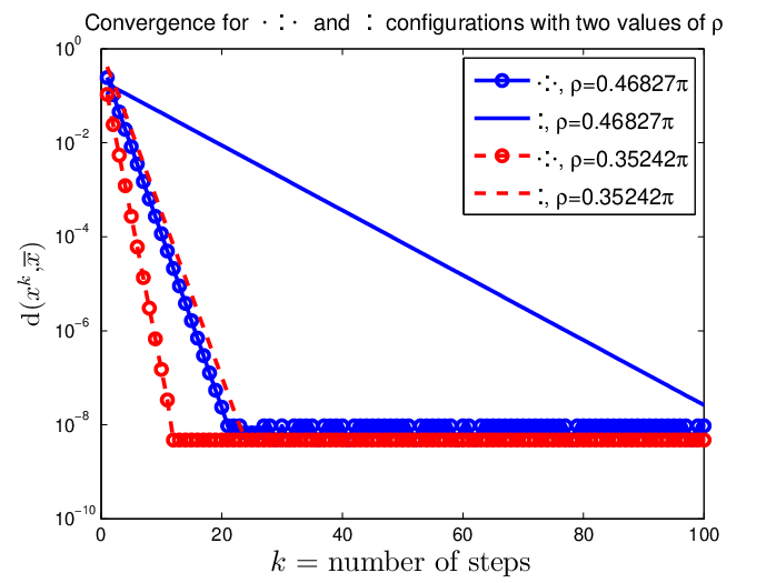
We consider the case of constant curvature since in this case the eigenvalues of the Hessian of the distance function are the same along all directions but the radial direction. Furthermore, let us assume is a -dimensional simply connected manifolds with constant curvature, that is where or (with the convention ). We construct two simple configurations for which Algorithm 1 converges very fast and very slowly, respectively. Consider four data points and the closed ball , where . Assume and are on the boundary of the ball in antipodal positions and that and are also in antipodal positions such that the geodesic from to and the geodesic from to are perpendicular at . We denote this configuration by . Obviously, is the center of mass of with equal weights. It is easy to verify that for the configuration the Hessian of at both along and along has eigenvalue . Consequently, at the ratio of the smallest and largest eigenvalue is , hence around ; and therefore, one expects that the local rate of convergence will be very fast. The opposite configuration is , that is, when and coincide with and , respectively. In this case, at along the Hessian of has eigenvalue of and in the perpendicular direction it has eigenvalue . Therefore, if , we have around which, in particular, can be very small if is close to . If , we have , which again can be small if is large. It is well known that the shape of the level sets of a function in a neighborhood of a minimizer is related to the ratio . If the level sets are very elongated or thin, this means that the Hessian has very small eigenvalues along longitudinal directions and very large eigenvalues along the lateral directions and hence can be very small. For our two configurations, we encourage the reader to compare the shapes of the level sets of in for levels close to (especially when is close to ) with the level sets of in for levels close to when is very large).
As a tangible example, on the standard unit sphere we run Algorithm 1 for both the configurations with two different values of and . The initial condition is chosen randomly. The step-size is chosen as . Figure 3 shows the distance in terms of the iteration index . It is clear that for the configuration the convergence is slower than the convergence for the configuration, and as increases, convergence for both configurations becomes slower. However, for the configuration as approaches , the convergence becomes extremely slow and the configuration is much more robust in that sense. Note that when even the center of mass of the configuration is on the verge of non-uniqueness and this causes further (error) sensitivity and hence poor convergence (see [2] on the issue of high noise-sensitivity of the Riemannian mean in positively curved manifolds).
Although our example is rare in statistical applications, in a more general setting also one expects that if the configuration of data points is such that the convex hull of the data points has an elongated shape (especially if the length of the convex hull is large), then locating the Riemannian center of mass becomes a difficult problem (with the exception of the Euclidean case). Our analysis does not tell the whole story in the case of non-constant curvature and we need more detailed analysis that takes into account the variability of eigenvalues of the Hessian of the distance function along non-radial directions, as well.
6. Concluding Remarks
Our goal has been to give and prove the the best possible conditions for convergence of the popular constant step-size gradient descent for finding the Riemannian center of mass. We argued that Conjecture 2.15 gives such best conditions (in some specific yet general sense). The proof of the conjecture seems to be difficult, because, in particular, it appears that such a proof requires some very deep understanding about the behavior of the exponential map of a Riemannian manifold. We proved the conjecture for manifolds of constant nonnegative curvature and our proof was based on comparison Theorem 3.1 which seems to give a better estimate of the behavior of the exponential map than what (possibly) could be gained by standard comparison theorems. Therefore, extending this comparison theorem (in appropriate sense) to manifolds of variable curvature not only could help prove Conjecture 2.15, but also could provide deeper understanding of the behavior of the exponential map of a general manifold. Our Theorems 4.1 and 4.2 (whose proofs are based on simple observations) give weaker convergence conditions, but still these results are considerably better than the available ones. Finer analysis could improve the results of these theorems, as well.
References
- [1] P.-A. Absil, R. Mahony, and R. Sepulchre. Optimization Algorithms on Matrix Manifolds. Princeton University Press, Princeton, NJ, 2008.
- [2] B. Afsari. Means and Averaging on Riemannian Manifolds. PhD thesis, University of Maryland, College Park, Dec. 2009.
- [3] B. Afsari. Riemannian center of mass: Existence, uniqueness, and convexity. Proc. Amer. Math. Soc., 139:655–673, 2011.
- [4] M. Arnaudon, C. Dombry, A. Phan, and L. Yang. Stochastic algorithms for computing means of probability measures. arXiv:1106.5106v1, 2011.
- [5] M. Arnaudon and F. Nielsen. On approximating the Riemannian 1-center. arXiv:1101.4718v1, 2011.
- [6] M. Berger. A Panoramic View of Riemannian Geometry. Springer, 2007.
- [7] A. Bhattacharya. Nonparametric Statistics on Manifolds with Applications to Shape Spaces. PhD thesis, The University of Arizona, 2008.
- [8] R. Bhattacharya and V. Patrangenaru. Large sample theory of intrinsic and extrinsic sample means on manifolds. I. Ann. Statist., 31(1):1–29, 2003.
- [9] S. R. Buss and J. P. Fillmore. Spherical averages and application to spherical splines and interpolation. ACM Transcations on Graphics, 20(2):95–126, April 2001.
- [10] B. Charlier. Necessary and sufficient condition for the existence of a Fréchet mean on the circle. arXiv:1109.1986v1, 2011.
- [11] I. Chavel. Riemannian Geometry: A Modern Introduction. Cambridge University Press, 2nd, 2006.
- [12] J. Cheeger and D. Ebin. Comparison theorems in Riemannian geometry. AMS Chelsea Publishing, Providence RI, 2008.
- [13] P. T. Fletcher, S. Venkatasubramanian, and S. Joshi. The geometric median on Riemannian manifolds with application to robust atlas estimation. NeuroImage, 45(1):S143–S152, March 2009.
- [14] A. Goh, C. Lenglet, P. Thompson, and R. Vidal. A nonparametric Riemannian framework for processing high angular resolution diffusion images (HARDI). In IEEE International Conference on Computer Vision and Pattern Recognition, 2009.
- [15] D. Groisser. Newton’s method, zeros of vector fields, and the Riemannian center of mass. Adv. in Appl. Math., 33:95–135, Nov 2004.
- [16] D. Groisser. On the convergence of some Procrustean averaging algorithms. Stochastics, 77(1):31–60, February 2005.
- [17] K. Grove and H. Karcher. How to conjugate -close group actions? Math. Z., 132(1):11–20, March 1973.
- [18] T. Hotz and S. Huckemann. Intrinsic means on the circle: Uniqueness, locus and asymptotics. arXiv:1108.2141v1, 2011.
- [19] H. Karcher. Riemannian center of mass and mollifier smoothing. Comm. Pure Appl. Math., XXX:509–541, 1977.
- [20] H. Karcher. Global Differential Geometry, volume 27 of MAA Studies in Mathematics, chapter Riemannian Comparison Constructions, pages 170–222. The Mathematical Association of America, 1989.
- [21] D. G. Kendall, D. Barden, T. K. Carne, and H. Le. Shape and Shape Theory. Wiley Series In Probability And Statistics. John Wiley & Sons, 1999.
- [22] W. S. Kendall. Probability, convexity, and harmonic maps with small image I: Uniqueness and fine existence. Proc. Lond. Math. Soc., 61(2):371–406, 2 1990.
- [23] K. A. Krakowski. Geometrical Methods of Inference. PhD thesis, The University of Western Australia, Aug. 2002.
- [24] K. A. Krakowski, K. Hüper, and J. H. Manton. On the computation of the Karcher mean on spheres and special orthogonal groups. In H. Araújo and M. I. Ribeiro, editors, Workshop on Robotics and Mathematics (ROBOMAT 07), pages 119–124, Coimbra, Portugal, September 2007.
- [25] H. Le. Locating Fréchet means with application to shape spaces. Adv. in Appl. Probab., 33(2):324–338, July 2001.
- [26] H. Le. Estimation of Reimannian barycenters. LMS Journal of Computation and Mathematics, 7:193–200, 2004.
- [27] J. H. Manton. A globally convergent numerical algorithm for computing the centre of mass on compact Lie groups. In Proceedings of the Eighth International Conference on Control, Automation, Robotics and Vision, page 22112216, Kunming, China, December 2004.
- [28] W. J. M’Clellanp and T. Preston. A Treatise On Spherical Trigonometry, with numerous examples Part I. Macmillan And Co., 1886. Available at Google Books.
- [29] M. Moakher. Means and averaging in the group of rotations. SIAM Journal on Matrix Analysis and Applications, 24(1):1–16, 2002.
- [30] X. Pennec. Intrinsic statistics on Riemannian manifolds: Basic tools for geometric measurements. J. Math. Imaging Vision, 25(1):127–154, July 2006.
- [31] B. Polyak. Introduction to Optimization. Translations Series in Mathematics and Engineering. Optimization Software, 1987.
- [32] T. Sakai. Riemannian Geometry, volume 149. American Mathematical Society, 1996.
- [33] A. Sarlette and R. Sepulchre. Consensus optimization on manifolds. SIAM Journal of Control and Optimization, 2008. to appear.
- [34] R. Tron, R. Vidal, and A. Terzis. Distributed pose averaging in camera networks via consensus on . In International Conference on Distributed Smart Cameras, 2008.
- [35] P. Turaga, A. Veeraraghavan, and R. Chellappa. Statistical analysis on Stiefel and Grassmann manifolds with applications in computer vision. In IEEE conference on Computer Vision and Pattern Recognition (CVPR), pages 1–8, June 2008.
- [36] O. Tuzel, F. Porikli, and P. Meer. Pedestrian detection via classification on Riemannian manifolds. IEEE Transactions on Pattern Analysis and Machine Intelligence, 30(10):1713–1727, October 2008.
- [37] C. Udrişte. Convex Functions and Optimization Methods on Riemannian Manifolds. Mathematics and Its Applications. Kluwer Academic Publishers, 1994.
- [38] L. Yang. Riemannian median and its estimation. LMS Journal of Computations and Mathematics, 13:461–479, 2010.
- [39] S-T. Yau. Non-existence of continuous convex functions on certain Riemannian manifolds. Mathematische Annalen, 207:269–270, 1974.