Two Algorithms for Orthogonal Nonnegative Matrix Factorization
with Application to Clustering

Let $M=(m_{1},\dots,m_{n})\in\mathbb{R}^{m\times n}_{+}$ be a nonnegative data matrix whose columns represent a set of $n$ points $\{m_{j}\}_{j=1}^{n}\in\mathbb{R}^{m}_{+}$. Solving the clustering problem means finding a set $\{\pi_{i}\}_{i=1}^{k}$ of $k$ disjoint clusters:

such that each cluster $\pi_{i}$ contains objects as similar as possible to each other according to some quantitative criterion. When choosing the Euclidean distance, we obtain the $k$-means problem, which can be formulated as follows [8]:

Equivalently, we can define a binary cluster indicator matrix $B\in\{0,1\}^{k\times n}$ as follows:

Disjointness of clusters $\pi_{i}$ means that rows of $B$ are orthogonal, i.e., $BB^{T}$ is diagonal. Therefore we can normalize them to obtain an orthogonal matrix $V=\{v_{ij}\}_{k\times n}=(BB^{T})^{-\frac{1}{2}}B$ (a weighted cluster indicator matrix) which satisfies the following condition:

It has been shown in [9] that the NMF problem with matrix $V$ satisfying condition (c1):

is equivalent to $k$-means. In fact, since $V$ in problem (2.2) is a normalized indicator matrix which satisfies $v_{ij}=|\pi_{i}|^{-\frac{1}{2}}\iff j\in\pi_{i}$, we have

which implies that, at optimality, each column $u_{i}$ of $U$ must correspond (up to a multiplicative factor) to a cluster centroid with $u_{i}=\sqrt{|\pi_{i}|}\,c_{i}=\frac{\sum_{j\in\pi_{i}}m_{j}}{\sqrt{|\pi_{i}|}}$ $\forall i=1,\dots,k$.

Let us now define a condition weaker than (c1):

It can be easily checked that $\eqref{c1}\Rightarrow\eqref{c2}$ while $\eqref{c2}\nRightarrow\eqref{c1}$. The difference between conditions (c1) and (2.2) is that condition (2.2) does not require the rows of $V$ to have their nonzero entries equal to each other. Now, if we only impose the weaker condition (2.2) on NMF, we obtain a relaxed version of (2.2) which, by definition, corresponds to orthogonal NMF:

In the following, we show the equivalence of problem (2.3) with a particular weighted variant of the spherical $k$-means problem:

The claim is that (2.3) and (2.4) are equivalent, i.e., a solution of (2.3) is obtained from a solution of (2.4) by means of elementary arithmetic operations, and vice-versa.

First, without loss of generality, we assume that $k$ is sufficiently small so that the solutions $U$ of (2.3) do not have vanishing columns. We then redefine “$U\geq 0$” (resp. “$V\geq 0$”) to mean that $U$ (resp. $V$) is nonnegative without vanishing columns (resp. rows). This redefinition does not alter the the solutions of (2.3).

Observe that (2.3) is equivalent to the following problem obtained by imposing the unit-norm constraint on the columns $\{u_{i}\}_{i=1}^{k}$ of $U$ instead of the rows of $V$:

Indeed, since the function $\psi:(U,V)\mapsto(UD^{-1},DV)$ with $D=\text{diag}(\|u_{1}\|,\dots,\|u_{k}\|)$ is a homeomorphism from the feasible set of (2.3) onto the feasible of (2.5) that does not modify the objective value, it is readily seen that if $(U,V)$ is a solution of (2.3), then $\psi(U,V)$ is a solution of (2.5); proving the reverse direction is equally straightforward.

It remains to show equivalence between (2.5) and (2.4). We say that a partition $\pi=\{\pi_{i}\}_{i=1}^{k}$ and a matrix $V$ (with $k$ rows) are compatible, which we write $V\sim\pi$, if the inclusion $j\in\pi_{i}$ holds whenever $V_{ij}\neq 0$. Using this notion, we first notice the crucial fact that $V\sim\pi$ for some $\pi$ if and only if each column of $V$ has at most one nonzero element (at position $(i,j)$ where $i$ is determined by $\pi_{i}\ni j$). Defining $\mathcal{V}$ to be the feasible set for $V$ in (2.5), it is now clear that $V\sim\pi$ and $V\geq 0$ imply that $V\in\mathcal{V}$ and that, in the reverse direction, one can easily check that $V\in\mathcal{V}$ implies the existence of a partition $\pi$ such that $V\sim\pi$.

We can now show that the following four propositions are equivalent, from which the main claim follows.

1. 1.

   $U$ and $V$ minimize $\|M-UV\|_{F}^{2}$ subject to $U\geq 0$, $\|u_{i}\|=1\,\forall i$, $V\geq 0$, $(VV^{T})_{ij}=0\,\forall i\neq j$,
   and $\pi$ is obtained by elementary operations to satisfy $V\sim\pi$.

2. 2.

   $U$, $V$, and $\pi$ minimize $\|M-UV\|_{F}^{2}$ subject to $U\geq 0$, $\|u_{i}\|=1\,\forall i$, $V\geq 0$, $V\sim\pi$.

3. 3.

   $U$, $V$, and $\pi$ minimize $\sum_{i=1}^{k}\sum_{j\in\pi_{i}}\|m_{j}-u_{i}v_{ij}\|^{2}$ subject to $U\geq 0$, $\|u_{i}\|=1\,\forall i$, $V\geq 0$, $V\sim\pi$.

4. 4.

   $U$ and $\pi$ maximize $\sum_{i=1}^{k}\sum_{j\in\pi_{i}}\left(m_{j}^{T}u_{i}\right)^{2}$ subject to $U\geq 0$, $\|u_{i}\|=1\,\forall i$,
   and $V$ is obtained by the elementary operations

   $$\begin{cases}v_{ij}=0&\text{if $j\notin\pi_{i}$}\\ v_{ij}=m_{j}^{T}u_{i}&\text{if $j\in\pi_{i}$}.\end{cases}$$

The equivalence between 1 and 2 follows from the discussion in the previous paragraph. The equivalence between 2 and 3 follows from a rewriting of the objective function made possible by the constraints.

Finally, the equivalence between 3 and 4 is established as follows. Referring to 3, given a feasible $U$ and $\pi$, we have for each term $\|m_{j}-u_{i}v_{ij}\|^{2}$ that the optimal $v_{ij}^{*}$ is given by:

(Observe that $m_{j}^{T}u_{i}\geq 0$ in view of the nonnegativity of $M$ and $U$.) Backsubstituting the optimal coefficients (2.6) in 3, we have that $U$ and $\pi$ of 3 minimize the function

Hence they maximize the function

This shows that 3 implies 4, and the converse is readily established by contradiction.

It is insightful to compare formulation (2.4) of ONMF with the spherical $k$-means problem [2], which is a variant of $k$-means where both data points and centroids are constrained to have unit norm:

Note that both problems (2.4) and (2.8) relate to maximizing the cosines of the angles between $u_{i}$ and the data points from the corresponding cluster. However, we observe that:

• •

  Because of coefficients $||m_{i}||^{2}$, problem (2.4) is sensitive to the norm of the data points, as opposed to spherical $k$-means (2.8) which only depends on their direction;

• •

  Even for normalized data points (i.e., $||m_{i}||=1$ $\forall i$), problem (2.4) is similar but not equivalent to spherical $k$-means (2.8) because it tries to maximize the sum of squares of the cosines (instead of their sum).

• •

  Contrarily to problem (2.4), spherical $k$-means (2.8) does not require nonnegativity of $u_{i}$’s, although it will clearly hold at optimality when data points $m_{j}$ are nonnegative.

Based on the analysis of ONMF from Section 2 (in particular, Theorem 2.1), we explain in this section in which situations ONMF should be preferred to $k$-means and spherical $k$-means. This issue can be settled by addressing the following two questions:

1. 1.

   Should scaling of the data points influence the cluster assignment?

   Given the cluster centroids, spherical $k$-means and ONMF are invariant to scaling in the sense that, for any $\alpha>0$, a data point $x$ and its scaling $\alpha x$ will be assigned to the same cluster (the one minimizing the angle between $x$ and the cluster centroid; see Section 2.4). On the contrary, $k$-means is very sensitive to scaling as it assigns data points to clusters based on distances; see Figure 1 for an illustration. In practice, there are many situations where cluster assignment should be independent of scaling so that spherical $k$-means and ONMF should be preferred to $k$-means. For example, in document classification, two documents discussing the same topic will roughly be multiple of one another (scaling depending then on the relative lengths of the documents), and, in hyperspectral imaging, pixels containing the same material will have their spectral signatures multiple of one another (scaling depending on the relative illumination conditions; see Section 4 for numerical experiments).

2. 2.

   Does the noise added to each data point depend on its norm?

   Spherical $k$-means is invariant under normalization of the data points (see Equation (2.8)) while ONMF gives more importance to data points with larger norm. For example, if the noise added to each data point is independent of its norm, ONMF should be preferred. In fact, in that situation, data points with larger norm are relatively contaminated with less noise hence should be given more importance. Another example is when data points with larger norm are statistically more significant. This is usually the case for example in document classification: assuming that each document discusses only one topic and that each topic is a distribution over the words, longer documents represent a larger sample of the corresponding topic distribution and should be given more importance. (In fact, most document classification software typically discards very short documents: ONMF implicitly takes care of this issue by giving less importance to shorter documents.) In hyperspectral imaging, background pixels contain mostly noise and should not be given too much importance; hence ONMF should also be preferred in this situation.

Figure 1 displays a comparison between $k$-means, spherical $k$-means and ONMF on two simple examples.

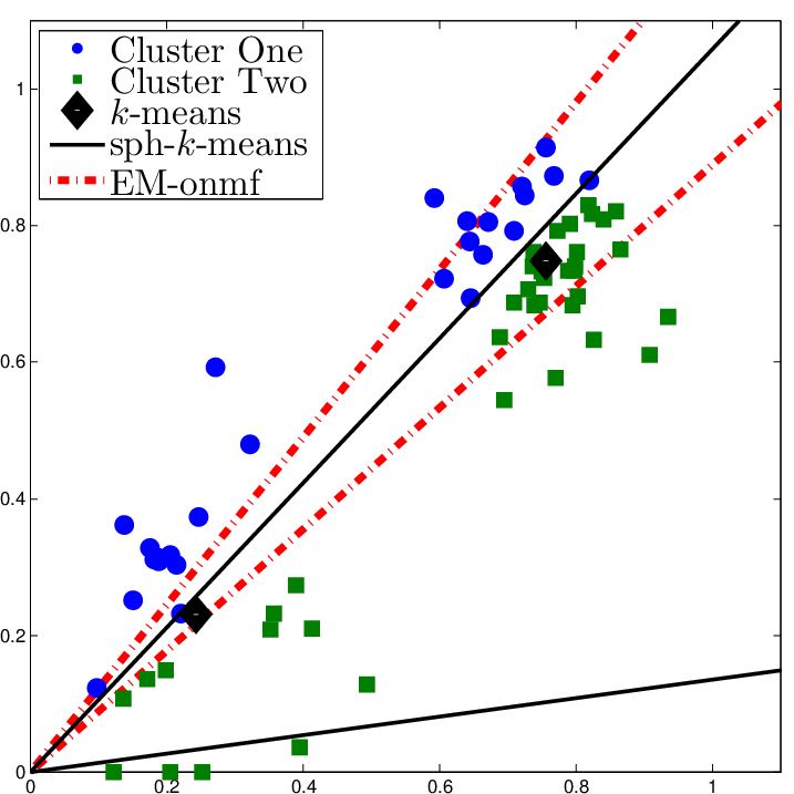
To conclude, ONMF should be preferred to both $k$-means and spherical $k$-means when

• (1)

  Scaling should not affect cluster assignment, and

• (2)

  Data points with larger norm are more reliable and should be given more importance.

To illustrate this, we generate several synthetic data sets as follows. Each data sets has six clusters $\{\pi_{i}\}_{i=1}^{6}$, each containing $100-(i-1)10$ data points for a total of $450$ data points. Each cluster centroid $u_{i}\in\mathbb{R}^{10}$ $1\leq i\leq 6$ is generated uniformly at random in the unit cube $[0,1]^{6}$. Each data point $m_{j}$ $1\leq j\leq 450$ is a multiple of its corresponding cluster centroid: $m_{j}=\alpha u_{k}$ where $\alpha>0$ is picked uniformly at random in the interval $[0.1,1]$. Hence, because of this scaling, $k$-means is not appropriate and will perform poorly. Each data point is then perturbed by some additive noise with fixed magnitude (i.e. independent of the norm of the data point, which should lead to ONMF performing better than spherical $k$-means). Concretely, each noise entry is drawn from a normal distribution with zero mean and fixed standard deviation $\epsilon$. Finally, the negative entries of each data point are set to zero to obtain a nonnegative input matrix (note that this can only reduce the noise). Letting $\{\pi^{\prime}_{i}\}_{i=1}^{6}$ be the clusters extracted by an algorithm and $\{\pi_{i}\}_{i=1}^{6}$ be the true clusters, the accuracy is defined as

where $[1,2,\dots,k]$ is the set of permutations of $\{1,2,\dots,k\}$. For each noise level $\epsilon\in[0,1]$, we generate ten synthetic data sets as described above, and Figure 2 reports the average accuracy of each algorithm using ten random initializations (except for ONMF which was solved using ONP-MF, which does not use random initialization, see Section 3).

As expected, we observe that ONMF outperforms $k$-means and spherical $k$-means. We will use the same synthetic data sets to compare the different ONMF algorithms in Section 4.

We present here a simple EM-like alternating algorithm designed to tackle the ONMF problem (2.3) based on its equivalence with the weighted variant of spherical $k$-means (2.4). It is very similar to the standard spherical $k$-means algorithm [2], except for the computation of cluster centroids. Specifically, it starts with an initial set of centroids, either randomly chosen or supplied as initial values. It then alternates between two steps:

1. 1.

   Given cluster centroids $\{u_{i}\}_{i=1}^{k}$, choose $\{\pi_{i}\}_{i=1}^{k}$ assigning each point to its closest cluster:

   	$\displaystyle j\in\pi_{i}\Rightarrow i$	$\displaystyle\in\operatornamewithlimits{argmax}_{1\leq\ell\leq k}{\left(m_{j}^{T}u_{\ell}\right)^{2}}$
   		$\displaystyle=\operatornamewithlimits{argmax}_{1\leq\ell\leq k}{\left(m_{j}^{T}u_{\ell}\right)}.$

   Notice that this step is exactly equivalent to the one of standard spherical $k$-means [2].

2. 2.

   Given the clustering $\{\pi_{i}\}_{i=1}^{k}$, compute the new optimal cluster centroids $\{u_{i}\}_{i=1}^{k}$ as follows. Define matrix $M_{i}\in\mathbb{R}^{m\times|\pi_{i}|}$ as the submatrix of $M$ containing the columns belonging to cluster $\pi_{i}$. We have to solve problem (2.7) with respect to the $u_{i}$’s:

   $$\max_{\{u_{i}\geq 0,||u_{i}||=1\}_{i=1}^{k}}\sum_{i=1}^{k}\sum_{j\in\pi_{i}}\left(m_{j}^{T}u_{i}\right)^{2}=\sum_{i=1}^{k}||M_{i}^{T}u_{i}||_{2}^{2}.$$

   There are $k$ independent problems: each $u_{i}$ must maximize the term $||M_{i}^{T}u_{i}||_{2}^{2}$. The optimal solution $u_{i}^{*}$ is given by the dominant left singular vector of $M_{i}$ associated with $\sigma_{1}(M_{i})$, the largest singular value of $M_{i}$:

   $$u_{i}^{*}=\operatornamewithlimits{argmax}_{||u||_{2}=1}||M_{i}^{T}u||_{2}^{2}=\operatornamewithlimits{argmax}_{||u||_{2}=1}u^{T}M_{i}M_{i}^{T}u,$$

   for which we have $||M_{i}^{T}u_{i}^{*}||_{2}=\sigma_{1}(M_{i})=||M_{i}||_{2}$. Moreover, since $M_{i}\geq 0$, the Perron-Frobenius theorem guarantees that $u_{i}^{*}$ can always be chosen to be nonnegative.

Algorithm 1, referred to as EM-ONMF, implements this procedure. We will see in the last section that, despite its simplicity, it works well for text clustering tasks.

Note that Algorithm 1 does not explicitly provide a solution to ONMF. However, a candidate solution of (2.5) can be obtained by taking $U=\begin{bmatrix}u_{1}&\dots&u_{k}\end{bmatrix}$ and selecting $V$ according to (2.6), from which a candidate solution of ONMF (2.3) is readily obtained as $(UD,D^{-1}V)$ where $D=\mathrm{diag}(\|V(1,:)\|_{2},\dots,\|V(k,:)\|_{2})$.

It is interesting to relate this with the original ONMF problem (2.5): given a partitioning $\{\pi_{i}\}_{i=1}^{k}$, let us denote $w_{i}=(v_{ij})_{j\in\pi_{i}}$ the subvector containing only the positive entries of the $i^{\text{th}}$ row of $V$. Then,

so that the optimal ($u_{i}$,$w_{i}$) must be an optimal solution of

Each of these problems looks for the best nonnegative rank-one approximation of a nonnegative matrix (i.e., a rank-one NMF problem). This in turn can be solved by combining the Eckart-Young and Perron-Frobenius theorems: taking the first rank-one factor generated by the singular value decomposition (SVD) (making sure it is nonnegative in case of non-uniqueness) leads to a minimum value for (2.10) equal to $||M_{i}||_{F}^{2}-\sigma^{2}_{1}(M_{i})$. Therefore, solving ONMF amounts to finding a partitioning $\{\pi_{i}\}_{i=1}^{k}$ such that the sum of squares of the first singular values of submatrices $M_{i}$’s is maximized, that is, ONMF problem (2.3) is equivalent to $\max_{\{\pi_{i}\}_{i=1}^{k}}\sum_{i=1}^{k}\sigma_{1}^{2}(M_{i})$.

In this section, we perform experiments on synthetic data sets as in Section 2.3 in order to compare the different ONMF algorithms. Figure 4 reports the average accuracy of each algorithm.

We observe that

• •

  ONP-MF or O-P(SVD)  perform the best among all ONMF algorithms. In particular, they are the only algorithms able to perfectly identify all clusters for small noise levels ($\epsilon=0.01$).

• •

  CHNMF, O-PNMF  and CH(SVD) perform similarly, their accuracies being in most cases lower than those of ONP-MF and O-P(SVD).

• •

  EM-ONMF performs rather poorly and is in general not able to perform a good clustering (although it is much faster than the other algorithms, see Table 1).

Table 1 gives for each algorithm the average computational time for one execution on a synthetic data set.

ONP-MF is slightly slower but typically obtains one of the best factorizations using only a single deterministic initialization.

We selected twelve well-known preprocessed document databases described in [21]. Each data set is represented by a term-by-document matrix of varying characteristics, see Table 2.

As a performance indicator, we use the accuracy; see Equation (2.9). We report the average value of the obtained accuracy along with the standard deviations in Table 3. For more than half of the data sets, the average best result was achieved by our algorithms, either EM-ONMF or ONP-MF. Moreover, our algorithms obtain the best performance among ONMF algorithms in ten out of the twelve data sets (being close for the two remaining data sets). While EM-ONMF is very fast with a low number of iterations (as the other EM-like algorithms), ONP-MF is in general slower than the other ONMF algorithms (especially CHNMF), and typically requires a larger number of iterations to converge.

Note that, in this paper, our focus is on the comparison of ONMF algorithms based on the Frobenius norm. Comparison with ONMF algorithms using other measures, such as the Kullback-Leibler divergence, and comparison with other topic models (such as LDA [3]) is a topic for further research.

A hyperspectral image is a set of images of the same object or scene taken at different wavelengths. Each image is acquired by measuring the reflectance (i.e., the fraction of incident electromagnetic power reflected) of each individual pixel at a given wavelength. The aim is to classify the pixels in different clusters, each representing a different material. We want to cluster the columns of a wavelength-by-pixel reflectance matrix so that each cluster (a set of pixels) corresponds to a particular type of material.

The swimmer image data set consists of 256 binary images of a body with four limbs which can be positioned in four different ways each. The goal is to find a part-based decomposition of these images, i.e., isolate the different constitutive parts of the images (the body and the limbs, 17 in total). Moreover, these parts are not overlapping, and therefore no rows of $V$ can share nonzero entries in the same column, and ONMF is an appropriate model. Figure 8 displays the basis elements obtained with the different ONMF algorithms. It can be observed that, in this case, the SVD-based initialization is of no benefit, neither for CHNMF nor for O-PNMF. All algorithms are able to successfully find the correct parts except O-PNMF  and O-P(SVD).

References

- [1] P.-A. Absil and J. Malick, Projection-like retractions on matrix manifolds, SIAM J. Optim., 22 (2012), pp. 135–158.
- [2] A. Banerjee, I. Dhillon, J. Ghosh, and S. Sra, Generative model-based clustering of directional data, in Proceedings of the ninth ACM SIGKDD International Conference on Knowledge Discovery and Data Mining (KDD-03), ACM Press, 2003, pp. 19–28.
- [3] D. Blei, A. Ng, and M. Jordan, Latent dirichlet allocation, Journal of Machine Learning Research, 3 (2003), pp. 993–1022.
- [4] L. Bottou, Online algorithms and stochastic approximations, in Online Learning and Neural Networks, D. Saad, ed., Cambridge University Press, 1998.
- [5] C. Boutsidis and E. Gallopoulos, Svd based initialization: A head start for nonnegative matrix factorization, Pattern Recognition, 41(4) (2008), pp. 1350–1362.
- [6] E. Chi and T. Kolda, On tensors, sparsity, and nonnegative factorizations, SIAM J. on Matrix Analysis and Applications, 33 (2012), pp. 1272–1299.
- [7] S. Choi, Algorithms for orthogonal nonnegative matrix factorization, in Proc. of the Int. Joint Conf. on Neural Networks, 2008, pp. 1828–1832.
- [8] I. Dhillon, Y. Guan, and B. Kulis, Weighted graph cuts without eigenvectors: A multilevel approach, IEEE Trans. on Pattern Analysis and Machine Intelligence, 29(11) (2007), pp. 1944–1957.
- [9] C. Ding and X. He, On the equivalence of nonnegative matrix factorization and spectral clustering, in Proc. of the Fifth SIAM Conference on Data Mining, 2005, pp. 606–610.
- [10] C. Ding, T. Li, W. Peng, and H. Park, Orthogonal nonnegative matrix tri-factorizations for clustering, in Proceedings of the Twelfth ACM SIGKDD International Conference on Knowledge Discovery and Data Mining, Philadelphia, PA, USA, August 20-23, 2006, 2006, pp. 126–135.
- [11] N. Gillis and R. Plemmons, Dimensionality Reduction, Classification, and Spectral Mixture Analysis using Nonnegative Underapproximation, Optical Engineering, 50, 027001 (2011).
- [12] Z. Guo, T. Wittman, and S. Osher, L1 unmixing and its application to hyperspectral image enhancement, in Proc. SPIE Conference on Algorithms and Technologies for Multispectral, Hyperspectral, and Ultraspectral Imagery XV, 2009.
- [13] R. Horn and C. Johnson, Matrix Analysis, Cambridge University Press, Cambridge, 1990.
- [14] J. Kim and H. Park, Fast nonnegative matrix factorization: An active-set-like method and comparisons, SIAM Journal on Scientific Computing, 6 (2011), pp. 3261–3281.
- [15] C.-J. Lin, Projected Gradient Methods for Nonnegative Matrix Factorization, Neural Computation, 19 (2007), pp. 2756–2779. MIT press.
- [16] J. Nocedal and S. Wright, Numerical Optimization, Second Edition, Springer, New York, 2006.
- [17] V. Pauca, J. Piper, and R. Plemmons, Nonnegative matrix factorization for spectral data analysis, Linear Algebra and its Applications, 406 (1) (2006), pp. 29–47.
- [18] F. Pompili, N. gillis, P.-A. Absil, and F. Glineur, Onp-mf: An orthogonal nonnegative matrix factorization algorithm with application to clustering, in 21st European Symposium on Artificial Neural Networks, Computational Intelligence And Machine Learning, 2013.
- [19] M. Winter, N-findr: an algorithm for fast autonomous spectral end-member determination in hyperspectral data, in Proc. SPIE Conference on Imaging Spectrometry V, 1999.
- [20] Z. Yang and E. Oja, Linear and nonlinear projective nonnegative matrix factorization, Trans. Neur. Netw., 21 (2010), pp. 734–749.
- [21] S. Zhong and J. Ghosh, Generative model-based document clustering: a comparative study, Knowledge and Information Systems, 8 (3) (2005), pp. 374–384.