Using Point to Set Correlations to Probe the Unjamming Transition

A length scale in overcompressed jammed packings that increases as they are decompressed (pressure $P\rightarrow 0$) is predicted from a bulk-surface argument. Based on counting arguments that date back to Maxwell[16], and more recently discussed in [6, 17], one begins with $M\left[z\right]/2$ force bearing contacts in a subregion of a packing, where $M$ is the number of grains in the subregion and $\left[z\right]$ is the average number of contacts per grain of the packing. For each of the $M$ grains, there are $dM$ equations of mechanical equilibrium (ME) constraining the forces at each of the $M\left[z\right]/2$ contacts (in $d$ dimensions). As is discussed below, in the limit of very stiff grains, the deformations of two grains in contact are impossible to resolve even though contacts can carry a great deal of force. The only constraints on these contact forces, then, are ME equations, and force laws can be ignored. There are $M\left[z\right]/2-dM=M\delta z/2$ unconstrained contact force magnitudes, which are taken to be the degrees of freedom, with $\delta z=\left[z\right]-z_{0}$. Finally, if one defines a subregion by a set of boundary grains, these grains provide an additional $A$ constraints from the boundary. Roughly, $A\propto\sqrt{M}$ in 2D. The number of grains can be estimated using the definition of the packing fraction:

The unitless length $R$ is the ratio of size of the subregion $L$ to the radius $r$ grains (for our purposes, systems are bidisperse and $r$ is taken to be the diameter of the smaller grain), and the parameter $c$ characterizes the polydispersity.

Using 1, the number of excess contact force degrees of freedom $\delta n$ can be written as a function of $R$. In 2D,

At this point, it’s worth contrasting the bulk-surface argument presented here with those found in the literature [5, 6]. In previous constructions of the bulk-surface argument, the boundary of the subregion is said to contribute a set of fixed, “frozen” contact forces, so that the total number of excess contacts $M\delta z/2$ is ${\it{\it reduced}}$ by $A$ contacts. This should be contrasted with the above construction, where the boundary term contributes ${\it additional}$ boundary constraints on the variable contact forces. Near isostaticity, there is no difference between the two constructions, but away from isostaticity, the boundary term in the formulation of [5, 6], when contributing extra frozen contacts, should scale with $z$: $A\propto\sqrt{M}\left[z\right]$, since on average there are more contacts on the boundary if there are more contacts in the packing as a whole.

Frozen contact forces differ from additional constraints due to ME: the former reduce the number of degrees of freedom [5, 6] and are proportional in number to $\left[z\right]$ while the latter serve to further determine the existing contact forces and are proportional in number to $M$. An important length scale is determined by $\delta n_{nom}\left(R_{0}\right)=0$. This length scale defines the size of the smallest region within which the mechanical equilibrium equations can be satisfied, and $R_{0}\propto\delta z^{-1}$ if one assumes that the dependence on $\phi$ is small. In the existing literature [5], this length scale, referred to as the isostatic length scale $l^{*}$, is deduced from a form of the bulk-surface argument that depends on frozen boundary contact forces. There is no difference in the results of the two constructions as $\delta z\rightarrow 0$. However, with boundary contact forces frozen, $l^{*}\sim\frac{\left[z\right]}{\delta z}$, and can differ significantly from $R_{0}$ at large overcompressions. In [4] the isostatic length scale is measured indirectly through the response to a point-force perturbation to mechanically stable overcompressed packings, and is shown to scales as $1/\delta z$. In later sections, it will be made clear why a bulk-surface argument of the form 2 is preferable in the context of the PTS correlation.

The vibrational spectrum of granular packings as defined by the dynamical matrix provides more insight into the nature of unjamming. The excess degrees of freedom $\delta z$ can be related to the pressure of the packing through the vibrational density of states[5, 18]. A critical frequency $\omega^{*}$ is associated with the highest energy debye-like mode of a marginally stable packing. Anomalous modes (modes whose density of states are roughly independent of the frequency) appear at energies higher than $\omega^{*2}$, and this energy difference is proportional to $-P$. So, the energy change due to an imposed pressure $P$ is $\Delta E\leq\omega^{*2}-AP$ and the critical frequency is $\omega^{*}\propto P^{1/2}$. To relate $\omega^{*}$ to the contact number, one must look at the characteristic size of the anomalous modes. It turns out that anomalous modes with $\omega\geq\omega^{*}$ are quasi-localized with localization length $\geq R_{0}$[19]. Assuming a linear dispersion relation $\omega\propto ck$, the critical frequency is: $\omega^{*}\propto\frac{1}{R_{0}}\propto\delta z$, and therefore, $\delta z\propto P^{1/2}$[20, 21].

It should be noted that the validity of the dynamical matrix approach to deriving the vibrational spectrum has been recently called into question[22]. Numerical studies show that in the limit of infinite system sizes, arbitrarily small perturbation amplitudes lead to contact breaking, and mixing of the eigenmodes of the dynamical matrix[22]. This result calls into question any analysis of response of jammed packings based on the vibrational density of states. While the result $\delta z\propto P^{1/2}$ is well established in simulations (we have verified that our numerics reproduce this result), the justification of this relationship relies on the existence of anomalous modes in the vibrational spectrum. Furthermore, the explanation that the length scale measured in collective response is associated with the extent of such anomalous modes becomes questionable, further motivating our choice to look for a static measure of a correlation length.

There are two aspects to the bulk-surface argument which are mean-field in nature. The first is the relation between $P$ and $\delta z$. In principle, $\Delta E$ should depend on factors which contain the force vector orientations, but it is assumed that these vectors are randomly distributed in the packing so that their effects on $\Delta E$ average to a constant. If, on the other hand, the local configuration of force vectors depended heavily on the orientations of nearby force vectors, as one might expect for instance simply because of the overlap constraints, this might not be a reasonable assumption. It turns out that at least for isotropically compressed packings, the packing geometry is sufficiently disordered that this assumption is sound[5].

The second mean-field assumption is built into the counting that goes into the bulk-surface argument. The assumption that the number of excess force degrees of freedom is given by the difference between the number of force variables and the number of ME equations requires that these equations are all independent, since a linear system has a number of undetermined variables equal to the difference between the total number of variables and the number of $\emph{independent}$ equations. As will be detailed in the sections below, this assumption does fail significantly as $P\rightarrow 0$.

The work of [3] on transverse grain displacement correlations in simulations of 2D disk packings under quasistatic shear strain reports a growing length scale for packing fractions below $\phi_{J}$. Interestingly, they find no evidence for a growing length scale as $\phi_{J}$ is approached from above. These results are consistent with continuum elastic theory [23] which shows that shear-strained packings can be thought of as random local forces applied to a homogeneous elastic sheet. Because of this homogeneity, the system size becomes the only relevant length scale of the system. Furthermore, in [24] a field-theoretic calculation of pressure fluctuation correlations for both isotropically compressed and sheared systems shows that such correlations exhibit a power-law behavior, with the only length scale emerging as the grain size, independent of the pressure.

At this point, it would seem that (2-point) stress correlations do not exhibit a growing length scale. Neither do displacement correlations, even though force fluctuations seem to scale with the isostatic length scale $l^{*}$. The latter requires one to consider the response to a point perturbation, and unlike systems in thermal equilibrium, the relation between response and correlations is not established in jamming systems. The question of whether there is a static correlation function that can be identified with the unjamming transition is, therefore, still wide open.

The importance of probing a static correlation function can be understood from contrasting the results from the non-equilibrium unjamming transition to that of, say, a simple Ising model: for a large enough system, a single spin configuration of the magnet equilibrated at some temperature $T$ will exhibit a spin-spin correlation length that grows as $T_{c}$ is approached. One does not have to consider properties of the dynamics which brings one spin configuration into another. If the unjamming transition is to be thought of as a critical point and not a kinetic freezing transition[25], a static correlation function must show a diverging length scale. In section 4 a new type of correlation function is discussed, which is specifically designed to overcome the added complexity of amorphous systems where critical behavior is still to be expected.

The Force Network Ensemble (FNE) has been studied extensively as a statistical mechanical model of granular matter[14]. While there are several variations on the model studied in the literature[28, 15, 13], the key assumption made when developing the FNE is that when grains are sufficiently rigid, infinitesimally small deformations of grains (or, simply deformations that are too small to observe experimentally) lead to significant fluctuations in the contact forces. With this assumption, the force law coupling grain deformations to forces is no longer relevant. For a given fixed configuration of mechanically stable grains (referred to here as an MS), the contact forces can take on any positive values that do not violate the constraints of mechanical equilibrium (ME). When the grains are frictionless, the forces $\vec{f}_{ij}$ always lie along the vector normal to the point of contact $\hat{r}_{ij}$, which in the case of disks is the center-to-center separation vector between grain $i$ and its neighbor $j$. The ME constraints are linear in the contact force magnitude, and are expressed as[29]:

The matrix $A$ is made up of the geometric information of the MS. In particular, it contains the components of $\hat{r}_{ij}$. The vector $\vec{f}$ is a list of contact force magnitudes $N$ long, where $N$ is the total number of contacts for the MS. The vector $\vec{f}$ represents a particular force ${\it network}$ that satisfies ME for a given MS, and should not be confused with a force vector $\vec{f}_{ij}$ that is applied to a particular grain. The vector $\vec{b}$ is a list of length $2M+3$ (in 2D) that contains the values of the constraints. Entries which correspond to force balance equations are zero, while the entries corresponding to components of the stress tensor are non-zero constants: $\vec{b}=\left(0,0\ldots\sigma_{xx},\sigma_{xy,}\sigma_{yy}\right)$.

The matrix $A$ of the linear system in Eq. 5 is rectangular with dimensions $2M+3$ by $N$ in 2D. A packing with periodic boundary conditions will result in two more constraints on the contact forces in 2D[14]. The istostatic argument of section 2 is easily expressed in terms of the shape of $A$: assuming that the equations of ME are all ${\it independent}$ (an assumption that will be discussed further in the proceeding sections) the packing is isostatic, and hence the linear system 5 is precisely ${\it determined}$, if A is square. If $A$ is rectangular with more rows than columns, the packing is hypostatic, and therefore Eq.5 ${\it overdetermined}$, and if $A$ is rectangular with more columns than rows, the packing is hyperstatic and therefore Eq.5 is ${\it underdetermined}$. For the case where Eq.5 is underdetermined, there is an infinite set of force networks $\left\{\vec{f}\right\}$ that satisfy ME for the given MS. This set makes up a force network ensemble for the given MS, referred to as the MS-FNE. It’s important to notice that two MS-FNE’s are not interchangeable; a set of force networks for a given geometry is not valid for any other geometry.

Sampling force networks for an amorphous geometry requires solving Eq.5. When the linear system is underdetermined, the matrix $A$ has a nullity greater than zero, and so the solutions of $A\vec{f}=\vec{0}$ are spanned by null space of dimension $\delta z$ (when $A$ is a full rank matrix). The singular value decomposition (SVD) of $A$ results in the basis $\left\{\hat{g}\right\}$ of the null space of $A$. Since Eq.5 is inhomogeneous, $\left\{\hat{g}\right\}$ are not solutions to Eq.5. Actually, $\left\{\hat{g}\right\}$ are solutions at exactly zero pressure, which requires each basis vector to have both positive and negative elements, violating the positivity constraint. The homogeneous solutions $\left\{\hat{g}\right\}$ must be added to a particular solution $\vec{f}_{0}$ which satisfies ME for the given MS and which satisfies the inhomogeneous constraints, including the components of the stress tensor. A good choice of $\vec{f}_{0}$ is easily found by applying a force law, for instance linear spring interactions which are used throughout this work, to construct a given MS and then extract a force network from the geometry. In summary, for all $\left\{\hat{g}\right\}$ such that $A\hat{g}=0$, there is a solution $\vec{f}=\vec{f}_{0}+c\hat{g}$ to Eq.5 for an amplitude $c$.

A method for sampling force networks for amorphous geometries then amounts to finding a particular MS using any packing protocol, solving for the null space of $A$ using numerical SVD routines, and choosing amplitudes $c$ at random to construct new force networks $\vec{f}$ from $\vec{f}_{0}$ and $\left\{\hat{g}\right\}$. As with the wheel move[28], which can be shown to be a particular null vector of the $A$ corresponding to the triangular lattice, the positivity constraint must be obeyed, and so any $\vec{f}=\vec{f}_{0}+c\hat{g}$ must be regected if the resulting $\vec{f}$ has any negative elements. This approach to sampling the FNE was first developed in [15].

It is not yet clear how to construct the PTS correlation function for granular systems. A procedure analogous to that of LJ glass formers might be to remove grains from a subregion of a packing and replace them with a configuration of grains that originates from another packing, and energy minimize to find the new mechanically stable packing while keeping the boundary grains fixed. This approach presents several issues. First, without thermal fluctuations it is not clear that the final state is in equilibrium. There are large energies associated with grain overlaps at the boundary. More fundamental though is the problem of defining the correlation function. Since relevant variables such as local stresses and forces are generally defined with respect to the individual grains or contacts, and number of grains and contacts can vary between subregions (as well as their locations), there is no clearly defined overlap. With the added machinery of the MS-FNE, though, a well-defined correlation function presents itself. For a given MS, we define a PTS correlation function probes the correlations between valid force networks that make up the FNE. The PTS correlation function $C$ is then well defined as the inner product of any valid force network $\vec{f}$ with the initial force network $\vec{f}_{0}$, normalized by the magnitudes of the force networks to guarantee that $C$ is never greater than 1: $C=\hat{f}_{0}\cdot\hat{f}$. But, this correlation function still is not a function of a boundary size $R$. Fortunately, the FNE allows for the ${\it net}$ force on a particular grain to be fixed to a value other than zero through the addition of inhomogeneous constraints to $A$. First, a boundary of size $R$ is defined on a subregion of the packing. For the work discussed here, the boundaries are always square to match the symmetry of the simulation box. Grains that are on the interior of the boundary are considered in force equilibrium. They contribute ME equations to $A$ which are homogeneous. Grains on the boundary, on the other hand, contribute inhomogeneous constraints to $A$; the neighbors of those boundary grains that are exterior to the boundary exert a fixed net force on the boundary grain. These exterior grains do not themselves contribute ME equations to $A$. All of the contact forces which are associated with grains that have centers which lie interior to the boundary are considered “free” and are allowed to fluctuate. Contacts outside of the boundary are not allowed to fluctuate and do not contribute to the columns of $A$ (see figure 2). The matrix $A$ now depends on the boundary size $R$. As $R$ increases, more grains and contact forces fall into the interior of the boundary, and so the dimensions of $A$ grow. In addition, the vector $\vec{b}$, which now depends on $R$ as well, will have entries corresponding to the fixed effective external forces being exerted on the boundary grains from their exterior neighbors. The matrix equation $A\left(R\right)\vec{f}\left(R\right)=\vec{b}\left(R\right)$ must now be solved using the approach outlined for sampling the MS-FNE. A well defined PTS correlation function can now be constructed so that it is dependent on the size of the boundary: $C\left(R\right)=\hat{f}_{0}\cdot\hat{f}\left(R\right)$.

As was discussed in section 3, the bulk-surface argument is chosen to have a boundary term which corresponds to the number of grains contributing ME equations to the constraints on the contact forces, rather than a count of the number of “frozen” contact forces. Here, a bulk-surface argument based on frozen contact forces would be an error. There is no way of fixing the contact forces at the boundary. Only ${\it net}$ ${\it forces}$ on each boundary grain can be fixed. Fixing contact forces would involve fixing elements of $\vec{f}$, which cannot be done given the approach to sampling the FNE described here, since there is no control over the particular values that the members of $\left\{\hat{g}\right\}$ can take when computing the SVD of $A$.

The correlation function $C\left(R\right)$ is computed by averaging over many force networks $\vec{f}\left(R\right)$ and, once a sufficient sampling of the FNE has been completed, the sampling is repeated for many MS. Averages over the FNE are identified with $\left\langle\ \right\rangle$ brackets, and quantities that are averaged over the set of MS are identified with $\left\langle\ \right\rangle_{g}$ brackets. Also, the size of the bounding box $R$ can be varied and the process repeated for different values of $R$. The only relevant microscopic scale is the grain diameter $D$, so in practice the parameter that is controlled is the scaled boundary size $R=R/D$. In the end, the correlation function studied here for disk packings is $\left\langle\left\langle C\left(R\right)\right\rangle\right\rangle_{g}=\left\langle\left\langle\hat{f}_{0}\cdot\hat{f}\left(R\right)\right\rangle\right\rangle_{g}$.

For systems of disk packings ranging from 30 to 900 grains in 2D, bidisperse with one third of the grains 1.4 times larger than the other two thirds[30, 31], $\left\langle\left\langle C\left(R\right)\right\rangle\right\rangle_{g}$ has been measured. The MS averaging is done over 40 packings. The FNE averaging is done over $10^{6}$ different forces networks. Force networks are found by creating a high dimensional random walk in the null space of solutions to $A\left(R\right)\vec{f}\left(R\right)=\vec{b}\left(R\right)$, with a random step size chosen from a uniform distribution on an interval $\left[-c,c\right]$ where $c$ is some fixed constant. The random walk always begins from the initial force network $\vec{f}_{0}$. In practice, a value of $c=0.05$ is found to keep the success rate of the sampling high (as few steps as possible violate the positivity constraint) while quickly moving away from the initial force network $\vec{f}_{0}$ for a wide range of overcompressions and system sizes. For the largest system size, figure 3 illustrates the trajectory of the random walk by calculating $C\left(R\right)=\hat{f}_{0}\cdot\hat{f}_{i}\left(R\right)$ for each random walk step $i$. When $R$ is changed, value of $C\left(R\right)=\hat{f}_{0}\cdot\hat{f}_{i}\left(R\right)$ quickly drops and fluctuates around some value for that $R$. This acts as a direct verification in terms of the correlation function that the force network sampling has been allowed enough time to “equilibrate,” and that the correlation function is measuring equilibrium properties of the FNE.

The results for $\left\langle\left\langle C\left(R\right)\right\rangle\right\rangle_{g}$ for the largest system size of 900 grains is shown in [7]. At small $R$, the correlation function is nearly 1, and at some value of $R$ it begins to decay. As will be discussed below, the tail is a power law in $R$, and does not produce a length scale. However, the crossover value of $R$ where the correlation function begins to decay does exhibit the characteristics of a critical length scale. This crossover value is referred to here as $R_{0}$ because of its relationship to the $R_{0}$ of the bulk-surface argument, which will be discussed in more detail below.

In addition, $\left\langle\left\langle C\left(R\right)\right\rangle\right\rangle_{g}$ appears to asymptote to some value greater than zero for large $R$. Subtracting off this asymptotic value $q_{0}=C\left(R=L/d\right)$, for linear system size $L$, one can define a connected correlation function $\left\langle\left\langle C\left(R\right)-q_{0}\right\rangle\right\rangle_{g}$. When $R$ is scaled by $R_{0}$, the connected correlation function collapses onto a master curve that decays rapidly to zero, a functional form which RFOT theory predicts for the PTS correlation function [8, 32].

Since $\delta n\left(R<R_{0}\right)=0$, there is no null space of $A\left(R\right)$. The correlation function $C\left(R\right)$ for $R<R_{0}$ is identically 1 since $C\left(R<R_{0}\right)=\hat{f}_{0}\cdot\hat{f}_{0}=1$. The length scale is extracted from the numerics by identifying that value of $R$ at which $\delta n\left(R\right)$ is first greater than zero (or the value of $R$ at which $C\left(R\right)$ is less than 1). As a function of $\left\langle P\right\rangle_{g}$, the geometry-averaged critical length $\left\langle R_{0}\right\rangle_{g}$ fits a power law. A linear fit of $ln\left(\left\langle R_{0}\right\rangle_{g}\right)$ as function of $ln\left(\left\langle P\right\rangle_{g}\right)$ establishes an exponent of $\nu=0.461\pm 0.012$ with a $95\%$ confidence interval for the largest (900 grain) packings (figure 5). The lowest overcompression, $\delta\phi=0.001$, is left out of the fit because nearly all of the geometries have $R_{0}=L$. The inclusion of $\delta\phi=0.001$ changes the exponent to $\nu=0.45\pm 0.015$. Either way, while the exponent is near the mean-field value of $0.5$, the difference is significant considering the confidence bounds.

The exponent is verified using finite size scaling. Since all of the numerical results are done at finite system sizes, the exponent that is observed in power law fits may be susceptible to system size effects. Furthermore, a length scale only truely diverges at a critical point in the infinite system limit, so establishing a length scale which becomes the system size in a finite system near the critical point begs the question, is this length finite at the critical point but just larger than any system size we have studied? The purpose of finite size scaling is to isolate the functional form of the length scale in the infinite system limit by scaling out the dependence on the system size. First assume a form

To better understand the deviation from mean-field, let’s return to the bulk-surface argument discussed in 3. The $R_{0}$ extracted from the numerics and used thus far in the discussion of the exponent $\nu$ is found by identifying $\delta n\left(R_{0}\right)=0$, where $\delta n$ is the nullity of the linear system that describes the subregion of the packing of size $R$ found from the SVD. Let’s define a nominal nullity $\delta n_{nom}$ which is simply $n\left(R\right)-m\left(R\right)$, where $n\left(R\right)$ is the number of contacts inside a boundary of size $R$ and $m\left(R\right)$ is the number of grains inside and on the boundary, so that $\delta n_{nom}$ is the expression for the mean field bulk-surface argument presented in Section 3. If the mean field approximation discussed in Section 3 is valid, the equality $\delta n=\delta n_{nom}$ should hold. In fact, $\delta n_{nom}$ does not equal $\delta n$, and what’s more, a $R_{0}^{nom}$ extracted from $\delta n_{nom}$ reproduces the mean-field result. Figures 5 and 6 also show the results for $R_{0}^{nom}$. Since so much of the data at low pressures saturate at the system size for $R_{0}^{nom}$, it is difficult to do a power law fit as with $R_{0}$, even for the largest system size. The power laws plotted for $R_{0}^{nom}$ are not taken from a fit. Instead, the exponent $0.5$ is verified using finite size scaling only. For small $M^{1/2\nu}\left\langle P\right\rangle_{g}$ none of the collapses do well. If one focuses only on the plateau and tail, the collapse for $\nu=0.46$ fails particularly in the plateau and near the knee, while $\nu=0.54$ fails in the tail. $\nu=0.5$ seems to be the best balance between the two. The finite size scaling for $R_{0}$ works well over a larger range, including the plateau.

As an additional test of the the finite size scaling collapse used to verify the exponent $\nu$, one can also focus on the tail of the collapse. In the tail, one expects $\left\langle R_{0}\right\rangle_{g}/M^{1/2}$ to exhibit a power law dependence on $M^{1/2\nu}\left\langle P\right\rangle_{g}$. If the exponent of this power law and the exponent used in the finite size scaling differ, this leads to a failure of the collapse at different system sizes. However, within the limits set by the variance in the data due to the sensitivity of the collapse on the exponent used, the tail of $\left\langle R_{0}\right\rangle_{g}/M^{1/2}$ should have a slope corresponding to the infinite system size exponent. This can be seen by assuming a power-law form for the scaling function, and using $\nu_{t}$ as the “test” exponent used to collapse the finite system size data:

The recovery of the mean-field exponent for $R_{0}^{nom}$ implies something very interesting about the bulk-surface argument. The mean-field result for $\delta n_{nom}$ as presented in Section 3 has a form $\alpha P^{1/2}R^{2}-\beta R$. Even if the nullity from SVD, $\delta n$, differed from $\delta n_{nom}$ by a term linear in $R$, the functional form of the length scale wouldn’t change. The difference in exponents for $R_{0}$ and $R_{0}^{nom}$ must be the result of a novel $P$ dependent term in the bulk-surface argument for $\delta n$: $\delta n-\delta n_{nom}=P^{-1/2}f\left(P^{1/2}\right)$ for some unknown function f. Figure 8 suggests that scaling forms for both $P^{1/2}\delta n$ and $P^{1/2}\delta n_{nom}$ exist and are functions of $\left\langle R\right\rangle_{g}\left\langle P^{1/2}\right\rangle_{g}$ only. But, the scaling form of $\delta n_{nom}$ is a quadratic over the entire data range, even below the cusp at $\left\langle R_{0}^{nom}\right\rangle_{g}\left\langle P^{1/2}\right\rangle_{g}$, while $\delta n$ fails to be quadratic near $\left\langle R_{0}\right\rangle_{g}\left\langle P^{1/2}\right\rangle_{g}$. Section 8 discusses four distinct sources of disagreement between $\delta n$ and $\delta n_{nom}$.

The set of solutions to Eq.5 sampled by the random walk make up a high dimensional vector space. Two separate but related spaces are discussed here. The more commonly discussed space is the “force space,” a $z$ dimensional space where each axis corresponds to a different contact force magnitude[13]. Not every point in this space is a solution. However, there are bounds on where solutions can be located in the force space. The positivity constraint confines all solutions to the $\left\{f_{1}...f_{z}\right\}\geq 0$ hyper-octant. Additionally, a linear global constraint, say from fixing the pressure, is generally applied to the FNE, so that there is at least one constraint of the form $\sum_{i=1}^{z}c_{i}f_{i}=C$, where the $c_{i}$’s and $C$ are some constants from the geometry of the packing, for instance the center-to-center separations of the disks for the pressure constraint. Ignoring the ME constraints for a moment, the linear global constraints require that at least one $f_{i}$ be non-zero. In principle, there can be solutions where $f_{i}=C$ while $f_{j\neq i}=0$. This provides the point of intercept with each axis of the force space. Since the global constraints are linear, each intercept is connected by a line, forming a high dimensional polygon (polytope).

Contained within this polytope are all of the valid force networks for the given MS, although much of the space within this polytope does not correspond to valid solutions. The vertices, for instance, which are the intercepts with the $f_{i}$ axes, cannot be solutions. They correspond to force networks where $f_{i}=C>0$ and $f_{j\neq i}=0$, which is never a force network that satisfies ME.

It is possible though to apply the ME constraints by further changing the shape and dimensionality of the polytope. Beginning with the polytope defined by only the global constraint and some valid force network, choose a ME constraint which is applied to grain $i$ with $z_{i}$ contacts. Such a constraint relates $z_{i}$ contact forces linearly, so it is represented geometrically as a $z_{i}$ dimensional (unbounded) polytope. Each ME constraint allows $f_{i}=0$ as a solution, so the ME polytopes intersect the origin. Therefore, an ME polytope is never entirely embedded in the global constraint polytope. Once imbedded in the force space, the intersection of ${\it all}$ such ME constraint polytopes with each other as well as the global constraint polytope represents the set of valid force networks. The polytope that results from these intersections contains what will be referred to as the “solution space,” equal in dimension to the nullity of $A$. The solution space is simply connected because of the linearity of the forces: the sum of any two force networks is also a valid force network, and properly normalized will satisfy the global constraint. The solution space is also likely convex; [13] claims that the force space is “trivially” convex, also due to the linearity, but fails to take into account the positivity constraint when coming to this conclusion. The positivity constraints have similar implications for the solution space: while linear superpositions of valid force networks do result in valid force networks, they do not necessarily result in contact forces which are all positive. However, an assumption of convexity allows us to estimate the number of valid force networks at a given pressure, as which we now explain in more detail.

Particular properties of the solution space are dependent on the MS. But, a useful approximation is that the solution space is enclosed by a hypersphere of dimension $\delta n$. Since, in FNE, each valid force network is considered to be equally likely, and the solution space is simply connected, the volume of the $\delta n$-dimensional hypersphere estimates the number of solutions. The radius of the hypersphere for solutions within a bounded region of linear size $R$ is $\left\langle\eta\left(R\right)\right\rangle$, the average distance from $\vec{f}_{0}\left(R\right)$ to a point on the hypersphere. When $\delta n>2$, a random walk through the solution space beginning at $\vec{f}_{0}\left(R\right)$ is transient; that is to say, the walker will rapidly approach the surface of the hypersphere, and spend the majority of its time there. This reflects the geometric property of high dimensional polytopes which is that the majority of the its volume is concentrated near the boundary. As the dimension $\delta n$ becomes larger, a good approximation of $\left\langle\eta\left(R\right)\right\rangle$ results from sampling $\vec{f}\left(R\right)-\vec{f}_{0}\left(R\right)$ over the random walk steps: $\left\langle\eta\left(R\right)\right\rangle=\left\langle\left|\vec{f}\left(R\right)-\vec{f}_{0}\left(R\right)\right|\right\rangle$. This is essentially a radius of gyration for the high-dimensional random walk, and a similar quantity has been used previously as a measure of force indeterminacy[15].

The volume of the hypersphere plays an essential role in the understanding of the unjamming transition as a critical point. As $R\rightarrow R_{0}$, the hypersphere shrinks, both in linear size $\left\langle\eta\left(R\right)\right\rangle$ and in dimension, to a single point that is the only solution to the precisely determined linear system of ME equations. Since, as shown earlier, $R_{0}$ becomes the system size as $P\rightarrow 0$, if the volume of the hypersphere is a measure of the number of valid force networks available, then the entropy of valid force networks goes to zero as $P\rightarrow 0$. The unjamming transition is associated with a point at which there are no solutions available to Eq.5.

In this section we’ll discuss a model of $\eta\left(R\right)$ and $C\left(R\right)$ based on properties of the solution space. These results will be based on two approximations, concerning the typical values for the “magnitudes” of the force networks:

The correlation function $C\left(R\right)$ is related to $\eta\left(R\right)$, which can be seen by expanding $\eta\left(R\right)^{2}=\left|\vec{f}\left(R\right)-\vec{f}_{0}\left(R\right)\right|^{2}$:

The approximate form of the correlation function also explains a peculiar property of the measurements of $\left\langle\left\langle C\left(R\right)\right\rangle\right\rangle_{g}$ from section 6: the correlation function does not decay to zero. In the $R\rightarrow\infty$ limit, and in mean-field, $C\left(R\right)=\frac{1}{2}\left(1+\frac{2M}{z}\right)$, which is $1$ at the isostatic point but is never less than $1/2$. This is essentially the result of the positivity constraint. If contact forces could be negative, $\left[f\right]$ would be zero when contact forces were uncorrelated. The average must always be greater than zero for compressive forces. Comparison of Eq. 10 with numerical results are presented in section 9.

The deviation from the mean-field exponent of $\nu=0.5$ suggests that mean-field bulk-surface argument breaks down. In this section analysis of the behavior of $\eta\left(R\right)$ is used to identify a logarithmic correction to the mean-field prediction. The radius of gyration normalized by the force scale, $\bar{\eta}^{2}\left(R\right)=\eta^{2}\left(R\right)/\left[f\right]^{2}$, collapses for different values of $P$ according to the scaling form $\left\langle P\right\rangle_{g}^{1/2}\left\langle\bar{\eta}^{2}\left(R\right)\right\rangle_{g}=G\left(\left\langle R\right\rangle_{g}\left\langle P\right\rangle_{g}^{1/2}\right)$ (see figure 9).

The hypersphere that encloses the valid force networks has a dimensionality $\delta n\left(R\right)$, which has been shown (Eq.7) to depend on $\bar{\eta}\left(R\right)$. Furthermore, the linear size of the hypersphere is $\eta\left(R\right)$. In order for the volume of the hypersphere to be a count of solutions to $A\left(R\right)\vec{f}\left(R\right)=\vec{b}\left(R\right)$, the linear size must be unitless, and so the unitless volume $V\left(\left\langle\bar{\eta}\right\rangle_{g}\right)$ depends only on the average ${\it normalized}$ radius of gyration. The number of solutions $V\left(\left\langle\bar{\eta}\right\rangle_{g}\right)$ approaches 1 as $\left\langle\eta\right\rangle$ decreases; the hypersphere shrinks in size and in dimension. But, there is always a single solution to ME, even at the isostatic point (where the linear system is precisely determined). Therefore, the entropy $\ln\left(V\left(\left\langle\bar{\eta}\right\rangle_{g}\right)\right)$ goes to zero when $\left\langle\bar{\eta}\right\rangle_{g}$ goes to some small value $\bar{\eta}_{0}$.

It should be mentioned that $\bar{\eta}_{0}$ only has an interpretation as an MS-averaged value. For any particular MS, $\bar{\eta}$ is always zero when $R<R_{0}$. But, over many geometries at a particular $\left\langle P\right\rangle_{g}$, the value of $R_{0}$ can fluctuate, and so $\left\langle\bar{\eta}\right\rangle_{g}$ is only zero when $R=0$. On the other hand, the volume of the hypersphere $V\left(\left\langle\bar{\eta}\right\rangle_{g}\right)$ becomes 1 at a value of $\left\langle R\right\rangle_{g}$ larger than zero since it is a function of $\left\langle\bar{\eta}\right\rangle_{g}$ and not $\bar{\eta}$. This value of $\left\langle R\right\rangle_{g}$ corresponds to a value of $\left\langle\bar{\eta}\right\rangle_{g}$ which is greater than zero, but which controls the entropy-vanishing behavior of the solution space, and it is this value of $\left\langle\bar{\eta}\right\rangle_{g}$ that is being referred to as $\bar{\eta}_{0}$ (see figure 10).

Next we look more closely at the scaling function $G\left(\left\langle R\right\rangle_{g}\left\langle P\right\rangle_{g}^{1/2}\right)$. For small values of $y=\left\langle R\right\rangle_{g}\left\langle P\right\rangle_{g}^{1/2}$, the scaling function is fitted well by $G\left(y\right)=G_{0}e^{-\left(b/y\right)^{\alpha}}$, for fitting parameters $\alpha$, $G_{0}$, and $b$ (see caption for figure 9). At $\left\langle\bar{\eta}\right\rangle_{g}=\bar{\eta}_{0}$, the form of the scaling function implies

The following sections explore some microscopic origins for the failure of the bulk-surface argument by analyzing the statistics of some microscopic properties of the MS configurations, as well as some sample packing geometries and the null spaces of their corresponding linear systems.

The first correction to the mean-field bulk-surface argument results from the vectorial nature of the ME equations. Unlike most constraint satisfaction problems, where each vertex or node contributes a single constraint on the variables which correspond to links associated with that vertex, with ME multiple equations describe force balance, further coupling the force degrees of freedom. Specifically, in 2D, there are two force balance equations associated with each grain. If a grain has only one force exerted on it, that force variable is $\emph{overdetermined}$. One equation is all that is necessary to solve for the force variable, and the other equation is not necessary. This single force variable is known and is effectively not a variable at all. In 2D, the same happens when a grain has two force variables. The two equations of ME can be used to define both force variables. Only grains with three or more contacts are undetermined. In a packing without a fixed boundary, there are never grains with less than three contacts. However, when there is a boundary defined by a set of additional boundary constraints, grains with only one or two force variables are possible (see figure 12).

At low pressure the effect of the boundary grains which involve one or two force variables also tend to completely define the contact forces of neighboring grains. This allows for the phenomenon of effectively defining force variables near the boundary to propagate into the interior of the subregion, and at lower pressures this effect propagates further into the interior (see figure 11). A recursive algorithm is used to find these effectively determined force variables. All of the grains with two or less force variables are found, and then all remaining grains, with two or less forces after taking into account these effectively determined forces, are found. This process is repeated until all effectively determined force variables are found.

These effectively determined forces and corresponding ME equations both contribute corrections to the bulk-surface argument. The dependence of these corrections is roughly linear as a function of $R$, but the slope has a dependence on $P$ (figure 13).

While the local corrections to the bulk-surface argument are the most important contributions to the bulk-surface argument, they are not the only corrections. A second important correction comes from isostatic clusters of grains which are embedded inside the boundary of size $R$. Generally, there are sometimes one (or more) connected sets of grains within the boundary who’s ME equations together define a linear system which completely determines the corresponding set of force variables. This set of grains is not necessarily the entire set of grains within the subregion (if it was, the nullity would be zero). In addition, linear subsystems embedded within these isostatic clusters are typically underdetermined, meaning that the linear subsystems defined by these clusters cannot be reduced to local effects like those due to the corrections discussed previously.

In addition to having a $P$ dependence, these cluster contributions to the bulk-surface argument are not linear in $R$, but do exhibit scaling with the pressure (figure 15).

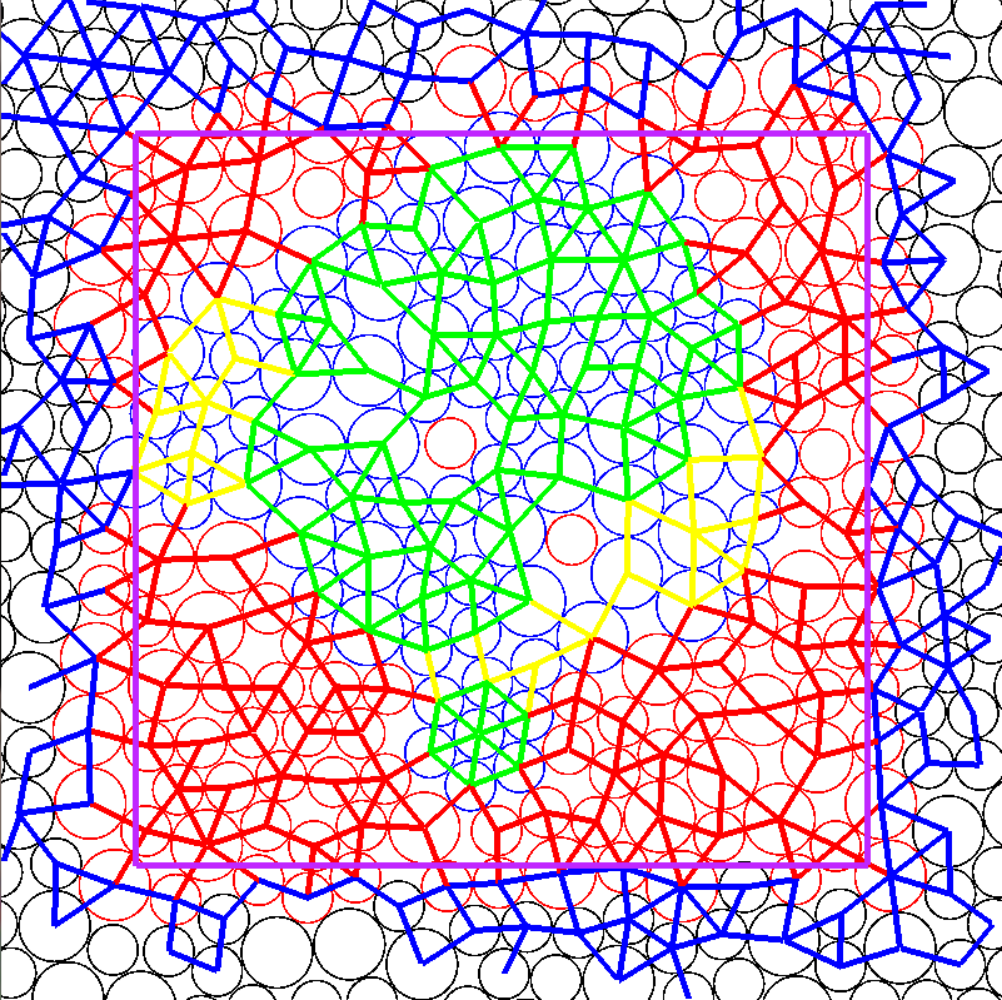
The combination of locally determined force variables and isostatic clusters occasionally leads to a fracturing of the subregion defined by $R$ into multiple underdetermined clusters (i.e., clusters of force variables which can be changed while satisfying ME). A third, and less important, correction results from the number of distinct underdetermined clusters. To be clear, these clusters are $\emph{not}$ the yellow isostatic clusters. For each cluster of underdetermined forces, the set of determined boundary forces defines a local stress tensor. Because this stress tensor is fixed as long as the boundary forces cannot change, the three components (in 2D) of the stress tensor provide additional relationships between the otherwise independent equations of ME which make up the linear system associated with the underdetermined cluster, reducing the total number of independent equations by three. These fractured subregions do not occur frequently enough to be characterized statistically in a quantitative way, but they clearly become more common as the pressure is lowered.

A simple algorithm is employed to count the number of independent clusters. First, the algorithm chooses a grain which is undetermined (meaning a grain whose ME equations are not involved in either a locally determined or an isostatic cluster). Then, it builds a set of grains out of this first grain’s neighbors, and repeats this process with the new grains until the set includes the neighbors of each other grain in the set or a boundary grain, which has all determined forces. Then the algorithm restarts with a grain not included in the previous set. It continues to build these new sets until all of the undetermined grains have been exhausted. The number of times the algorithm restarts is the number of independent clusters.

Finally, even after the previously discussed corrections to be bulk-surface argument are taken into account, there are very rarely special cases where a single force variable shared by two grains can be determined (in the sense that it is already known), even though none of the other force variables associated with those grains are. This may seem counter intuitive. All of the previously discussed phenomena involve a boundary effect where a grain whose force variables are all determined is in contact with a grain whose force variables are not all determined. At first, it might seem that if all of a grain’s contact force variables can change but one, there is no reason why that one should not fluctuate as well. In the special case of crystalline order, though, we know from experience with the “wheel move” that the ME equations are not all independent, leading to additional “breathing” modes. Take, for instance, the localized wheel move type cluster in the bottom of figure 17. There are 14 ME equations associated with this cluster, and including the two yellow links which point upward (and are shared between grains which also contain undetermined force variables, which is what makes this example unique) there are 14 force variables. Assuming the two vertical links do indeed correspond to determined variables, the wheel move still allows for the 12 internal green links to fluctuate without changing any of the other forces, simply because of the added symmetry of the triangular lattice. Or, to put it another way, because the ME equations associated with a crystalline structure are not all independent, some forcs must be determined and the SVD essentially “chooses” to localize the basis on the crystalline structure and never allow the boundary force variables to fluctuate. Because the wheel move is in some sense a different underdetermined cluster, it does count towards the total number of underdetermined clusters. But, since it is not separated from the main cluster by determined grains, only some particularly fortuitous determined forces, it is not detected by the cluster detection discussed in 8.

It is not enough to simply have crystalline structure; the crystalline structure must be surrounded by fixed forces as well, or there would not be an independent set of stress tensor constraints on the cluster and so would be indistinguishable from the main cluster. As a result, these wheel move clusters appear to be extremely rare; too uncommon, in fact, to allow for meaningful statistics.

In figure 18 the difference between $\delta n$ and $\delta n_{nom}$ is shown. The difference $\delta n-\delta n_{nom}$ represents the total correction to the bulk-surface argument, which takes the form $\delta n_{nom}=aR^{2}P^{1/2}-bR$ for constant $a$ and $b$ (the effects of slight variations in packing fraction are being ignored). The correction $\gamma(R,P)=\delta n-\delta n_{nom}$ amounts to an additional term in the bulk-surface argument: $\delta n=aR^{2}P^{1/2}-bR+\gamma(R,P)$. If this term were to be either linear and independent of pressure, or quadratic and dependent on the square root of pressure, the mean-field exponent $\nu=0.5$ would be recovered. As seen in figure 18, neither is the case. $\gamma(R,P)$ is linear in $R$, with a slope of $P^{-1/4}$, and a pressure dependent vertical intercept $Y\left(P\right)$.The bulk-surface argument, then, has a form $\delta n=aR^{2}P^{1/2}-(b-P^{-1/4})R+Y(P)$, which does not have a root of $R_{0}\propto P^{-1/2}$. Even though there is no theory predicting this form for $\delta n$, it’s worth noting that RFOT would predict a free energy as a bulk-surface competition with a temperature dependent surface tension [9] (in analogy to the pressure dependent coefficient of the linear term found here).

This section is concluded with an illustration of the clusters that emerge in a single packing as the pressure is lowered (figure 19). The figure caption addresses the particular characteristics of each step in the decompression.

References

- [1] AJ Liu and SR Nagel. Nonlinear dynamics - jamming is not just cool any more. Nature, 396(6706):21–22, 1998.
- [2] CS O’Hern et al. Jamming at zero temperature and zero applied stress: The epitome of disorder. Phys. Rev. E, 68(1, Part 1):011306, 2003.
- [3] C. Heussinger and J-L Barrat. Jamming transition as probed by quasistatic shear flow. Phys. Rev. Lett., 102:218303, 2009.
- [4] Wouter G. Ellenbroek et al. Critical scaling in linear response of frictionless granular packings near jamming. Phys. Rev. Lett., 97(25):258001, 2006.
- [5] M Wyart et al. Effects of compression on the vibrational modes of marginally jammed solids. Phys. Rev. E, 72(5, Part 1):051306, 2005.
- [6] AV Tkachenko and TA Witten. Stress propagation through frictionless granular material. Phys. Rev. E, 60(1):687–696, 1999.
- [7] M Mailman and B Chakraborty. Signature of a thermodynamic phase transition in jammed granular packings: growing correlations in force space. Journal of Statistical Mechanics: Theory and Experiment, 2011(07):L07002, 2011.
- [8] J P Bouchaud and G Biroli. On the adam-gibbs-kirkpatrick-thirumalai-wolynes scenario for the viscosity increase in glasses. J. Chem. Phys, 121(15):7347–7354, 2004.
- [9] G. Biroli et al. Thermodynamic signature of growing amorphous order in glass-forming liquids. Nature Physics, 4(10):771–775, 2008.
- [10] Jean Philippe Bouchaud and G. Biroli. Rfot review. ArXiv:0912.2542, 2009.
- [11] Andrea Cavagna et al. Mosaic multistate scenario versus one-state description of supercooled liquids. Phys. Rev. Lett., 98(18):187801, 2007.
- [12] Andrea Montanari and Guilhem Semerjian. Rigorous inequalities between length and time scales in glassy systems. J. Stat. Phys., 125(1):22–54, 2006.
- [13] JH Snoeijer et al. Ensemble theory for force networks in hyperstatic granular matter. Phys. Rev. E, 70(6, Part 1):061306, 2004.
- [14] Brian P. Tighe et al. The force network ensemble for granular packings. Soft Matter, 6(13):2908–2917, 2010.
- [15] S McNamara and H Herrmann. Measurement of indeterminacy in packings of perfectly rigid disks. Phys. Rev. E, 70(6, Part 1):061303, 2004.
- [16] JC Maxwell. On the Calculation of the Equilibrium and Stiffness of Frames. Philosophical Magazine, 27:294–299, 1864.
- [17] CF Mouzarkel. Proceedings of Rigidity Theory and Applications Traverse City MI. Fundamental Material Science Series, Plenum, New York, 1998.
- [18] LE Silbert et al. Vibrations and diverging length scales near the unjamming transition. Phys. Rev. Lett., 95(9):098301, 2005.
- [19] Zorana Zeravcic, Wim van Saarloos, and David R. Nelson. Localization behavior of vibrational modes in granular packings. EPL (Europhysics Letters), 83(4):44001, 2008.
- [20] M Wyart. On the Rigidity of Amorphous Solid and Price Fluctuations, Conventions and Microstructure of Financial Markets. PhD thesis, SPEC, CEA Sarclay, Paris, 2005.
- [21] WG Ellenbroek. Response of Granular Media near the Jamming Transition. PhD thesis, University of Leiden, 2007.
- [22] Schreck C. F. et al. Jammed particulate systems are inherently nonharmonic. ArXiv:1012.0369, 2010.
- [23] C. E. Maloney. Correlations in the elastic response of dense random packings. Phys. Rev. Lett., 97(3), 2006.
- [24] Gregg Lois et al. Stress correlations in granular materials: An entropic formulation. Phys. Rev. E, 80:060303 (R), 2009.
- [25] David Chandler and Juan P. Garrahan. Dynamics on the Way to Forming Glass: Bubbles in Space-Time. In Annual Review of Physical Chemistry, VOL 61, volume 61 of Annual Review of Physical Chemistry, pages 191–217. 2010.
- [26] J. P. Bouchaud. Granular media: some ideas from statistical physics. In J.-L. Barrat, J. Dalibard, M. Feigelman, and J. Kurchan, editors, Slow Relaxations and Nonequilibrium Dynamics in Condensed Matter. Springer, Berlin, 2003.
- [27] K. Huang. Statistical Mechanics, Second Edition. John Wiley and Sons, New York, 1987.
- [28] BP Tighe et al. Force distributions in a triangular lattice of rigid bars. Phys. Rev. E, 72(3, Part 1):031306, 2005.
- [29] SI Newton. The Mathematical Principles of Natural Philosophy. Royal Society of London, London, 1687.
- [30] DN Perera and P Harrowell. Stability and structure of a supercooled liquid mixture in two dimensions. Phys. Rev. E, 59(5, Part B):5721–5743, 1999.
- [31] RJ Speedy. Glass transition in hard disc mixtures. Journal of Chem. Phys., 110(9):4559–4565, 1999.
- [32] M Dzero et al. Activated events in glasses: The structure of entropic droplets. Phys. Rev. B, 72(10):100201, 2005.
- [33] Silke Henkes and Bulbul Chakraborty. Statistical mechanics framework for static granular matter. Phys. Rev. E, 79(6, Part 1), 2009.
- [34] Aleksandar Donev, Robert Connelly, Frank H. Stillinger, and Salvatore Torquato. Underconstrained jammed packings of nonspherical hard particles: Ellipses and ellipsoids. Phys. Rev. E, 75(5, Part 1), 2007.