Holonomic gradient method for the distribution function of the largest root of a Wishart matrix

Hiroki Hashiguchi ^†^†thanks: Graduate School of Science and Engineering, Saitama University Yasuhide Numata ^†^†thanks: Department of Mathematical Informatics, Graduate School of Information Science and Technology, University of Tokyo^†^†thanks: JST CREST Nobuki Takayama ³³footnotemark: 3 ^†^†thanks: Department of Mathematics, Kobe University Affiliation: and Akimichi Takemura²²footnotemark: 2 ³³footnotemark: 3

January 2012

Abstract

We apply the holonomic gradient method introduced by Nakayama et al. [23] to the evaluation of the exact distribution function of the largest root of a Wishart matrix, which involves a hypergeometric function ${}_{1}\kern-0.50003ptF_{1}$ of a matrix argument. Numerical evaluation of the hypergeometric function has been one of the longstanding problems in multivariate distribution theory. The holonomic gradient method offers a totally new approach, which is complementary to the infinite series expansion around the origin in terms of zonal polynomials. It allows us to move away from the origin by the use of partial differential equations satisfied by the hypergeometric function. From numerical viewpoint we show that the method works well up to dimension 10. From theoretical viewpoint the method offers many challenging problems both to statistics and $D$ -module theory.

Keywords and phrases: $D$ -modules, Gröbner basis, hypergeometric function of a matrix argument, zonal polynomial

1 Introduction

For multivariate distribution theory in statistics, the theory of zonal polynomials and hypergeometric functions of matrix arguments, introduced by A.T. James and other authors, was a very important development in the 1950’s. They allowed explicit expressions of density functions and cumulative distribution functions of basic test statistics under non-null cases. Zonal polynomials are based on the representation theory of real general linear group and they possess many interesting combinatorial properties. Properties and applications of zonal polynomials and hypergeometric functions of matrix arguments are surveyed in Gross and Richards [5] and Richards [25]. Zonal polynomials are special cases of Jack polynomials, whose properties have been intensively studied by many mathematicians. See for example Chapters VI and VII of Macdonald [18] and Stanley [29]. Jack polynomials are further generalized to Macdonald polynomials (see, e.g., Kuznetsov and Sahi [17]).

Zonal polynomials and hypergeometric functions of matrix arguments are important and difficult to compute in non-null cases rather than the null case, where the covariance matrix is a multiple of the identity matrix. In the null case there are several approaches to obtain the distribution function or moments. Recent representative approach is to use the random matrix theory (RMT) and the landmark study on the connection between RMT and multivariate analysis was conducted by Johnstone [12], Johnstone [13]. Butler and Paige [2] proposed a method to compute the exact null distributions based on their Pfaffian representation given by Gupta and Richards [6].

Despite the above nice mathematical properties of zonal polynomials and hypergeometric functions of matrix arguments, from practical viewpoint they were not really useful for computations. Coefficients of zonal polynomials can be computed only through nontrivial combinatorial recursions. Although very ingenious recursion algorithms have been recently developed (Koev and Edelman [14]), computing zonal polynomials of large degrees remains to be a difficult problem because of inherent combinatorial complexities. Also, the convergence of infinite series expansion of hypergeometric functions of a matrix argument in terms of zonal polynomials was found to be slow (Muirhead [21], Hashiguchi and Niki [7]). Since the expansion of the hypergeometric function in terms of zonal polynomials is the expansion at the origin, the convergence for large values of the argument is necessarily slow.

The holonomic gradient method allows us to move away from the origin by the use of partial differential equations. Thus our approach provides a promising new method for attacking a longstanding problem in multivariate statistics. Our holonomic gradient method is, in spirit, on the track of the holonomic systems approach to combinatorial identities by Zeilberger [36]. Note that the series expansion and our holonomic gradient method are in fact complementary methods, because our method needs the series expansion for obtaining initial values for the partial differential equations.

The main purpose of this paper is to verify the performance of holonomic gradient method for ${}_{1}\kern-0.50003ptF_{1}$ . We found that a straightforward implementation of the holonomic gradient method works well for dimensions up to 10.

Butler and Wood [3] showed that the Laplace method gives a very good approximation to ${}_{1}\kern-0.50003ptF_{1}$ even for a high dimension, e.g., $m=32$ . However the Laplace method needs a peaked density function, which corresponds to a large degrees of freedom. Our method is an exact method, where the errors only come from discretization in numerically solving differential equations and the accuracies in the initial values. Hence our method works even for small degrees of freedom.

The organization of this paper is as follows. In Section 2 we summarize preliminary facts on the exact distribution of the largest root of a Wishart matrix. In particular we state the partial differential equation for ${}_{1}\kern-0.50003ptF_{1}$ by Muirhead [20]. In Section 3, for expository purposes, we fully describe our holonomic gradient method for dimension two. In Section 4 we derive properties of Pfaffian system for general dimensions. The Pfaffian system is a system of partial differential equations and is called an integrable connection in some literatures. Results of symbolic computations are presented in Section 5 and results of numerical experiments are presented in Section 6. We end the paper with discussion of open problems in Section 7.

2 Preliminaries

Let $\kappa=(k_{1},\dots,k_{l})\vdash k$ be a partition of a non-negative integer $k$ and define the Pochhammer symbol $(a)_{\kappa}$ by

\displaystyle(a)_{\kappa}=\prod_{i=1}^{l}\left(a-\frac{i-1}{2}\right)_{k_{i}},\quad(a)_{k_{i}}=\prod_{j=1}^{k_{i}}(a+j-1)\ \ \ ((a)_{0}=1).

Let ${{\cal C}_{\kappa}(Y)}$ denote the (“ $C$ -normalization” of) zonal polynomial indexed by $\kappa$ of an $m\times m$ symmetric matrix $Y$ . It is a homogeneous symmetric polynomial of degree $k$ in the characteristic roots $y_{1},\dots,y_{m}$ of $Y$ , satisfying $\sum_{\kappa\vdash k}{\cal C}_{\kappa}(Y)=(\mathop{\rm tr}Y)^{k}$ . For zonal polynomials in statistics see, e.g., James [10], Muirhead [22], Takemura [34] and Mathai et al. [19]. A hypergeometric function of a matrix argument is defined (Constantine [4]) as

{}_{p}\kern-0.50003ptF_{q}(a_{1},\dots,a_{p};c_{1},\dots,c_{q};Y)=\sum_{k=0}^{\infty}\sum_{\kappa\vdash k}\frac{(a_{1})_{\kappa}\dots(a_{p})_{\kappa}}{(c_{1})_{\kappa}\dots(c_{q})_{\kappa}}\frac{{\cal C}_{\kappa}(Y)}{k!}.

(1)

In this paper we study holonomic gradient method for ${}_{1}\kern-0.50003ptF_{1}(a;c;Y)$ . Let $I_{m}$ denote the $m\times m$ identity matrix and let $|X|$ denote the determinant of $X$ . For $\Re a>(m+1)/2$ , $\Re(b-a)>(m+1)/2$ , ${}_{1}\kern-0.50003ptF_{1}(a;c;Y)$ has the following integral representation

{}_{1}\kern-0.50003ptF_{1}(a;c;Y)=\frac{\Gamma_{m}(b)}{\Gamma_{m}(a)\Gamma_{m}(c-a)}\int_{0<X<I_{m}}\exp(\mathop{\rm tr}XY)|X|^{a-(m+1)/2}|I_{m}-X|^{c-a-(m+1)/2}dX,

(2)

where $0<X<I_{m}$ means that $X$ and $I_{m}-X$ are positive definite, $dX=\prod_{i\leq j}dx_{ij}$ is the Lebesgue measure of the upper triangular entries of $X$ , and

\Gamma_{m}(a)=\pi^{\frac{1}{4}m(m-1)}\prod_{i=1}^{m}\Gamma\left(a-\frac{i-1}{2}\right).

The hypergeometric function ${}_{1}\kern-0.50003ptF_{1}$ satisfies the the following Kummer relation (see (2.8) of Herz [8], (51) of James [10]):

\exp(-\mathop{\rm tr}Y){}_{1}\kern-0.50003ptF_{1}(a;c;Y)={}_{1}\kern-0.50003ptF_{1}(c-a,c;-Y).

(3)

Note that (2) implies that ${}_{1}\kern-0.50003ptF_{1}$ is an entire function in $Y$ .

The cumulative distribution function of the largest root $\ell_{1}$ of the $m\times m$ Wishart matrix $W$ with $n$ degrees of freedom and the covariance matrix $\Sigma$ is written as follows

\Pr[\ell_{1}<x]=C\exp\left(-\frac{x}{2}\mathop{\rm tr}\Sigma^{-1}\right)x^{\frac{1}{2}nm}{}_{1}\kern-0.50003ptF_{1}\left(\frac{m+1}{2};\frac{n+m+1}{2};\frac{x}{2}\Sigma^{-1}\right),

(4)

where

C=\frac{\Gamma_{m}\left(\frac{m+1}{2}\right)}{2^{\frac{1}{2}nm}(\det\Sigma)^{\frac{1}{2}n}\Gamma_{m}\left(\frac{n+m+1}{2}\right)}.

This follows from the results in Section 9 of Constantine [4] and the Kummer relation (3). See also Sugiyama [31].

The following partial differential equations for ${}_{1}\kern-0.50003ptF_{1}(a;b;Y)$ were derived by Muirhead [20].

Theorem 1 (Theorem 5.1 of Muirhead [20], Theorem 7.5.6 of Muirhead [22]).

The hypergeometric function $F={}_{1}\kern-0.50003ptF_{1}(a;c;Y)$ of a matrix argument $Y=\mathop{{\rm diag}}(y_{1},\dots,y_{m})$ is the unique solution of the following set of $m$ partial differential equations

	$\displaystyle\left[y_{i}\,\partial_{i}^{2}+\left\{c-\frac{m-1}{2}-y_{i}+{1\over\,2\,}\sum_{j=1,j\neq i}^{m}\frac{y_{i}}{y_{i}-y_{j}}\right\}\partial_{i}-{1\over\,2\,}\sum_{j=1,j\neq i}^{m}\dfrac{y_{j}}{y_{i}-y_{j}}\partial_{j}-a\right]$	$\displaystyle F=0,$		(5)
		$\displaystyle(i=1,\dots,m),$

subject to the conditions that $F$ is symmetric in $y_{1},\dots,y_{m}$ and $F$ is analytic at $Y=0$ , $F(0)=1$ .

The partial differential equation (5) has singularities along $y_{i}=0$ and $y_{j}=y_{i}$ , $j\neq i$ . However since $F$ is an entire function, $F$ is determined by the partial differential equations on the open region ${\cal X}=\{y\in\mathbb{C}^{m}\mid\prod_{i=1}^{m}y_{i}\prod_{i\neq j}(y_{i}-y_{j})\neq 0\}$ . In this paper we call ${\cal X}$ the non-diagonal region. Using

\frac{y_{i}}{y_{i}-y_{j}}=1+\frac{y_{j}}{y_{i}-y_{j}}

we can rewrite (5) as $g_{i}F=0$ , $i=1,\dots,m$ , where

g_{i}=y_{i}\partial_{i}^{2}+(c-y_{i})\partial_{i}+{1\over\,2\,}\sum_{j=1,j\neq i}^{m}\frac{y_{j}}{y_{i}-y_{j}}(\partial_{i}-\partial_{j})-a

(6)

is a differential operator annihilating $F$ . In our holonomic gradient method we make a direct use of the partial differential equations for numerical evaluation of ${}_{1}\kern-0.50003ptF_{1}$ .

3 Holonomic gradient method for dimension two

In this section we illustrate the holonomic gradient method for the case of $m=2$ . Although our purpose is to implement an algorithm of our method for a larger dimension, for clarity it is best to do “by hand” calculation for the case of $m=2$ . As in the previous section we simply write $F(Y)={}_{1}\kern-0.50003ptF_{1}(a;c;Y)$ .

In Nakayama et al. [23] the holonomic gradient method was used to obtain the maximum likelihood estimate. The reciprocal of the likelihood function was minimized and the method was called the holonomic gradient descent. For the application of this paper we simply use the holonomic gradient method for evaluating $F$ . Hence we omit the term “descent”. Also, for minimization, at each step of the iteration, a direction for increments was chosen to decrease the value of the function. In our application, starting from the origin $Y=0$ , we can choose arbitrary path to the target value $Y$ where we want to evaluate $F(Y)$ .

Another minor difference of the expository explanation in this section from Nakayama et al. [23] and Sei et al. [28] is that we use the simple forward Euler method (e.g., Section 3.1 of Ascher and Petzold [1]) for updating partial derivatives of $F$ . In Nakayama et al. [23], once an updating direction is chosen at each step of the iteration, the 4-th order Runge-Kutta method was used. The simple Euler method is used only for the purpose of exposition. It is easier to explain the basic idea of the holonomic gradient method with the simple Euler method. In our actual implementation in Section 6 we use the Runge-Kutta method for numerically solving the differential equation.

We will reduce our problem to a traditional problem of numerical analysis of an ordinary differential equation (ODE). For the reduction we utilize the notion of holonomic differential equations and the gradients of their solutions. It is why we call our method holonomic gradient method.

In the following we discuss the case of $y_{1}\neq y_{2}$ and $y_{1}=y_{2}$ separately.

3.1 Holonomic gradient method for non-diagonal region

In this subsection we assume $y_{1}\neq y_{2}$ . Two partial differential equations in (6) are written as

	$\displaystyle\Big[y_{1}\partial_{1}^{2}+(c-y_{1})\partial_{1}+\frac{1}{2}\frac{y_{2}}{y_{1}-y_{2}}(\partial_{1}-\partial_{2})-a\Big]F$	$\displaystyle=0,$		(7)
	$\displaystyle\Big[y_{2}\partial_{2}^{2}+(c-y_{2})\partial_{2}+\frac{1}{2}\frac{y_{1}}{y_{2}-y_{1}}(\partial_{2}-\partial_{1})-a\Big]F$	$\displaystyle=0.$		(8)

Suppose that we want to evaluate a higher derivative $\partial_{1}^{n_{1}}\partial_{2}^{n_{2}}F=\partial_{2}^{n_{2}}\partial_{1}^{n_{1}}F$ of $F$ . Let $n_{2}\geq 2$ . Then by (8)

\partial_{1}^{n_{1}}\partial_{2}^{n_{2}}F=\partial_{1}^{n_{1}}\partial_{2}^{n_{2}-2}\big(-\frac{c}{y_{2}}\partial_{2}+\partial_{2}-\frac{1}{2}\frac{y_{1}}{y_{2}(y_{2}-y_{1})}(\partial_{2}-\partial_{1})+\frac{a}{y_{2}}\big)F.

(9)

Noting

\partial_{2}\frac{1}{y_{2}}=-\frac{1}{y_{2}^{2}},\quad\partial_{2}\frac{y_{1}}{y_{2}(y_{2}-y_{1})}=-\frac{y_{1}(2y_{2}-y_{1})}{y_{2}^{2}(y_{2}-y_{1})^{2}},

for $n_{2}>2$ , the right-hand side of (9) is further written as

		$\displaystyle\partial_{1}^{n_{1}}\partial_{2}^{n_{2}-3}\Big(\frac{c}{y_{2}^{2}}\partial_{2}-\frac{c-y_{2}}{y_{2}}\partial_{2}^{2}+\frac{1}{2}\frac{y_{1}(2y_{2}-y_{1})}{y_{2}^{2}(y_{2}-y_{1})^{2}}(\partial_{2}-\partial_{1})$
		$\displaystyle\qquad\qquad\ -\frac{1}{2}\frac{y_{1}}{y_{2}(y_{2}-y_{1})}(\partial_{2}^{2}-\partial_{1}\partial_{2})-\frac{a}{y_{2}^{2}}+\frac{a}{y_{2}}\partial_{2}\Big)F.$		(10)

Although the result is somewhat complicated, the important fact is that the total degree of differentiation $n_{1}+n_{2}$ on the left-hand side of (9) is decreased by one to $n_{1}+n_{2}-1$ in (10). As long as the degree of $\partial_{1}$ or $\partial_{2}$ is more than one, then we can recursively apply (7) or (8) to decrease the total degree of differentiation. It follows that for each $n_{1},n_{2}$ , there exist rational functions $h^{(n_{1},n_{2})}_{00},h^{(n_{1},n_{2})}_{10},h^{(n_{1},n_{2})}_{01},h^{(n_{1},n_{2})}_{11}$ in $(y_{1},y_{2})$ such that

\partial_{1}^{n_{1}}\partial_{2}^{n_{2}}F=h^{(n_{1},n_{2})}_{00}F+h^{(n_{1},n_{2})}_{10}\partial_{1}F+h^{(n_{1},n_{2})}_{01}\partial_{2}F+h^{(n_{1},n_{2})}_{11}\partial_{1}\partial_{2}F.

(11)

In this notation (7) is written as

	$\displaystyle\partial_{1}^{2}F$	$\displaystyle=\frac{a}{y_{1}}F-(\frac{c-y_{1}}{y_{1}}+\frac{1}{2}\frac{y_{2}}{y_{1}(y_{1}-y_{2})})\partial_{1}F+\frac{1}{2}\frac{y_{2}}{y_{1}(y_{1}-y_{2})}\partial_{2}F$
		$\displaystyle=h^{(2,0)}_{00}F+h^{(2,0)}_{10}\partial_{1}F+h^{(2,0)}_{01}\partial_{2}F\qquad(h^{(2,0)}_{11}\equiv 0).$		(12)

For a general dimension, (11) corresponds to the reduction by a Gröbner basis as discussed in Section 4.

For us the important case is $n_{1}=1,n_{2}=2$ . Since

\partial_{1}\frac{y_{1}}{y_{2}(y_{2}-y_{1})}=\partial_{1}\big(\frac{1}{y_{2}-y_{1}}-\frac{1}{y_{2}}\big)=\frac{1}{(y_{2}-y_{1})^{2}}

we have

	$\displaystyle\partial_{1}\partial_{2}^{2}F$	$\displaystyle=\partial_{1}\big(-\frac{c-y_{2}}{y_{2}}\partial_{2}-\frac{1}{2}\frac{y_{1}}{y_{2}(y_{2}-y_{1})}(\partial_{2}-\partial_{1})+\frac{a}{y_{2}}\big)F$
		$\displaystyle=\big(-\frac{c-y_{2}}{y_{2}}\partial_{1}\partial_{2}-\frac{1}{2}\frac{1}{(y_{2}-y_{1})^{2}}(\partial_{2}-\partial_{1})-\frac{1}{2}\frac{y_{1}}{y_{2}(y_{2}-y_{1})}(\partial_{1}\partial_{2}-\partial_{1}^{2})+\frac{a}{y_{2}}\partial_{1}\big)F.$

There is a term $y_{1}\partial_{1}^{2}$ on the right-hand side, into which we further substitute (7). Then (11) for $\partial_{1}\partial_{2}^{2}F$ is written as

$\displaystyle\partial_{1}\partial_{2}^{2}F$	$\displaystyle=\Big(-\frac{c-y_{2}}{y_{2}}\partial_{1}\partial_{2}-\frac{1}{2}\frac{1}{(y_{2}-y_{1})^{2}}(\partial_{2}-\partial_{1})-\frac{1}{2}\frac{y_{1}}{y_{2}(y_{2}-y_{1})}\partial_{1}\partial_{2}+\frac{a}{y_{2}}\partial_{1}$
	$\displaystyle\qquad-\frac{1}{2y_{2}(y_{2}-y_{1})}\big((c-y_{1})\partial_{1}+\frac{1}{2}\frac{y_{2}}{y_{1}-y_{2}}(\partial_{1}-\partial_{2})-a\big)\Big)F$
	$\displaystyle=\frac{a}{2y_{2}(y_{2}-y_{1})}F+\Big(\frac{3}{4}\frac{1}{(y_{2}-y_{1})^{2}}+\frac{a}{y_{2}}-\frac{c-y_{1}}{2y_{2}(y_{2}-y_{1})}\Big)\partial_{1}F$
	$\displaystyle\quad-\frac{3}{4}\frac{1}{(y_{2}-y_{1})^{2}}\partial_{2}F-\Big(\frac{c-y_{2}}{y_{2}}+\frac{1}{2}\frac{y_{1}}{y_{2}(y_{2}-y_{1})}\Big)\partial_{1}\partial_{2}F$
	$\displaystyle=h^{(1,2)}_{00}F+h^{(1,2)}_{10}\partial_{1}F+h^{(1,2)}_{01}\partial_{2}F+h^{(1,2)}_{11}\partial_{1}\partial_{2}F.$	(13)

Since $F$ is a symmetric function in $y_{1}$ and $y_{2}$ , $\partial_{1}^{2}\partial_{2}F$ is obtained by permuting $y_{1}$ and $y_{2}$ .

Let

\vec{F}=\begin{pmatrix}F\\ \partial_{1}F\\ \partial_{2}F\\ \partial_{1}\partial_{2}F\end{pmatrix}

denote the vector consisting of $F$ and its square-free mixed derivatives. Differentiate the components of $\vec{F}$ by $y_{1}$ and denote $\partial_{1}\vec{F}=(\partial_{1}F,\partial_{1}^{2}F,\partial_{1}\partial_{2}F,\partial_{1}^{2}\partial_{2}F)^{t}$ . Similarly define $\partial_{2}\vec{F}$ . Then by (12) and (13), $\partial_{i}\vec{F}$ , $i=1,2$ , are written as $\partial_{i}\vec{F}=P_{i}(Y)\vec{F}$ , where $P_{1}$ and $P_{2}$ are the following $4\times 4$ matrices with rational function entries

P_{1}(Y)=\begin{pmatrix}0&1&0&0\\ h^{(2,0)}_{00}&h^{(2,0)}_{10}&h^{(2,0)}_{01}&0\\ 0&0&0&1\\ h^{(2,1)}_{00}&h^{(2,1)}_{10}&h^{(2,1)}_{01}&h^{(2,1)}_{11}\end{pmatrix},\quad P_{2}(Y)=\begin{pmatrix}0&0&1&0\\ 0&0&0&1\\ h^{(0,2)}_{00}&h^{(0,2)}_{10}&h^{(0,2)}_{01}&0\\ h^{(1,2)}_{00}&h^{(1,2)}_{10}&h^{(1,2)}_{01}&h^{(1,2)}_{11}\end{pmatrix}.

The matrices $P_{1},P_{2}$ are called coefficient matrices of a Pfaffian system (an integrable connection) for $F$ (Nakayama et al. [23]). Note that $P_{2}$ is obtained from $P_{1}$ by permutation of $y_{1}$ and $y_{2}$ . If we know the values of the components of $\vec{F}$ at $Y=(y_{1},y_{2})$ , $y_{1}\neq y_{2}$ , then values at a nearby point $Y+\Delta Y=(y_{1}+\Delta y_{1},y_{2}+\Delta y_{2})$ can be approximated by the simple Euler method (i.e. linear approximation) as

	$\displaystyle\vec{F}(Y+\Delta Y)$	$\displaystyle\doteq\vec{F}(Y)+\Delta y_{1}\partial_{1}\vec{F}(Y)+\Delta y_{2}\partial_{2}\vec{F}(Y)$
		$\displaystyle=\vec{F}(Y)+\Delta y_{1}P_{1}(Y)\vec{F}(Y)+\Delta y_{2}P_{2}(Y)\vec{F}(Y).$		(14)

Now suppose that we want to evaluate $F(y_{1},y_{2})$ at a particular point $(y_{1},y_{2})$ with $y_{1}\neq y_{2}$ . If we know $\vec{F}(Y_{0})$ at some point $Y_{0}=(y_{1}^{(0)},y_{2}^{(0)})$ , $y_{1}^{(0)}\neq y_{2}^{(0)}$ , close to the origin, then we can choose an appropriate sequence of points $Y^{(l)}=(y_{1}^{(l)},y_{2}^{(l)})$ , $l=0,\dots,L$ , such that $(y_{1},y_{2})=(y_{1}^{(L)},y_{2}^{(L)})$ . Along the sequence we can use (14) to update $\vec{F}(Y^{(l)})$ and finally the first element of $\vec{F}(Y^{(L)})$ gives $F(y_{1},y_{2})$ .

Therefore it remains to consider how to obtain the initial values. Close to the origin we can use the definition (1) of ${}_{1}\kern-0.50003ptF_{1}$ . If $Y$ is very close to zero, then we only need zonal polynomials of low orders, whose explicit forms are known. Zonal polynomials up to the third order are as follows; ${\cal C}_{(1)}(Y)={\cal M}_{(1)}(Y)$ ,

\begin{pmatrix}{\cal C}_{(2)}(Y)\\ {\cal C}_{(1,1)}(Y)\end{pmatrix}=\begin{pmatrix}1&\dfrac{2}{3}\\[6.88889pt] 0&\dfrac{4}{3}\end{pmatrix}\begin{pmatrix}{\cal M}_{(2)}(Y)\\ {\cal M}_{(1,1)}(Y)\end{pmatrix},\quad\begin{pmatrix}{\cal C}_{(3)}(Y)\\ {\cal C}_{(2,1)}(Y)\\ {\cal C}_{(1,1,1)}(Y)\end{pmatrix}=\begin{pmatrix}1&\dfrac{3}{5}&\dfrac{2}{5}\\[6.88889pt] 0&\dfrac{12}{5}&\dfrac{18}{5}\\[5.16663pt] 0&0&2\end{pmatrix}\begin{pmatrix}{\cal M}_{(3)}(Y)\\ {\cal M}_{(2,1)}(Y)\\ {\cal M}_{(1,1,1)}(Y)\end{pmatrix},

(15)

where ${\cal M}_{\kappa}(Y)$ is the monomial symmetric polynomial associated with a partition $\kappa$ . Since $F(y_{1},y_{2})$ can be expanded as

	$\displaystyle F(y_{1},y_{2})$	$\displaystyle=1+\frac{(a)_{(1)}}{(c)_{(1)}}{\cal C}_{(1)}(Y)+\frac{1}{2!}\left(\frac{(a)_{(2)}}{(c)_{(2)}}{\cal C}_{(2)}(Y)+\frac{(a)_{(1,1)}}{(c)_{(1,1)}}{\cal C}_{(1,1)}(Y)\right)+\cdots$
		$\displaystyle=1+\frac{(a)_{(1)}}{(c)_{(1)}}{\cal M}_{(1)}(Y)+\frac{(a)_{(2)}}{2(c)_{(2)}}{\cal M}_{(2)}(Y)+\left(\frac{(a)_{(2)}}{3(c)_{(2)}}+\frac{2(a)_{(1,1)}}{3(c)_{(1,1)}}\right){\cal M}_{(1,1)}(Y)+\cdots,$		(16)

for an example, $\partial_{1}\partial_{2}F(0,0)$ is obtained as

\partial_{1}\partial_{2}F(0,0)=\dfrac{(a)_{2}}{3(c)_{2}}+\dfrac{2a(a-{1\over\,2\,})}{3c(c-{1\over\,2\,})}.

In a similar manner, we have

	$\displaystyle\partial_{1}F(0,0)=\partial_{2}F(0,0)=\frac{a}{c},\ \partial_{1}^{2}F(0,0)=\partial_{2}^{2}F(0,0)=\dfrac{(a)_{2}}{(c)_{2}},$
	$\displaystyle\partial_{1}^{2}\partial_{2}F(0,0)=\partial_{2}^{2}\partial_{1}F(0,0)=\dfrac{(a)_{3}}{5(c)_{3}}+\dfrac{4(a)_{2}(a-{1\over\,2\,})}{5(c)_{2}(c-{1\over\,2\,})}.$		(17)

These formulae can be obtained by a symbolic mathematics software, such as the routines for Jack polynomials in sage mathematics software system (Stein et al. [30]).

In order to obtain the initial value $\vec{F}(Y_{0})$ at $Y_{0}=(y_{1}^{(0)},y_{2}^{(0)})$ close to the origin, we can use the approximation

\vec{F}(y_{1}^{(0)},y_{2}^{(0)})\doteq\vec{F}(0,0)+y_{1}^{(0)}\partial_{1}\vec{F}(0,0)+y_{2}^{(0)}\partial_{2}\vec{F}(0,0).

(18)

We code the above procedure using deSolve package in the data analysis system R. We show a simple source program in Appendix B. In addition, since the zonal polynomials are easy to evaluate for $m=2$ , we also evaluate the series expansion of ${}_{1}\kern-0.50003ptF_{1}$ up to $k=150$ . As an example, we compute percentage points by two methods for the case of $n=3$ , $\Sigma={\rm diag}(1/2,1/4)$ . The following percentage points for $\ell_{1}$ agree in two methods to 6 digits.

50%	90%	95%	99%
1.63785	3.54999	4.31600	6.05836

Butler and Wood [3] proposed the Laplace approximation for ${}_{1}\kern-0.50003ptF_{1}$ and Koev and Edelman [14] proposed efficient algorithms for computing the truncation of ${}_{1}\kern-0.50003ptF_{1}$ . For $m=2,n=30$ and $\Sigma={\rm diag}(1/2,1/4)$ , Figure 1 shows an illustrative example; the Laplace approximation fails to give the upper probability and the approximation by the truncation rapidly converges to zero with partitions of degrees which are not sufficiently large. The distribution function by the holonomic gradient method is stable and accurate even when $x$ is large.

Refer to caption — Figure 1: $m=2,n=30,\Sigma={\rm diag}(1/2,1/4)$

3.2 Holonomic gradient method for the diagonal line

In the previous subsection we assumed $y_{1}\neq y_{2}$ to avoid singularity of the differential equations. However ${}_{1}\kern-0.50003ptF_{1}$ itself does not have singularities. Hence we should be able to derive some differential equation even for $y=y_{1}=y_{2}$ .

In (7) and (8) we can perform the limiting operation $y_{1}\rightarrow y_{2}=y$ using the l’Hôpital rule. Since $F$ is a symmetric function, at $(y,y)$ we have

\partial_{1}F(y,y)=\partial_{2}F(y,y).

Also $\partial_{1}^{2}F(y,y)=\partial_{2}^{2}F(y,y)$ . Hence by the l’Hôpital rule, in (7) we have

\lim_{y_{1}\rightarrow y_{2}=y}\frac{\partial_{1}F-\partial_{2}F}{y_{1}-y_{2}}=\partial_{2}^{2}F-\partial_{1}\partial_{2}F=\partial_{1}^{2}F-\partial_{1}\partial_{2}F.

Then (7) for at $(y,y)$ is written as

0=\left[y\partial_{1}^{2}+(c-y)\partial_{1}+\frac{y}{2}(\partial_{1}^{2}-\partial_{1}\partial_{2})-a\right]F=\left[\frac{3}{2}y\partial_{1}^{2}+(c-y)\partial_{1}-\frac{y}{2}\partial_{1}\partial_{2}-a\right]F.

(19)

Based on this we derive an ODE for $f(y)=F(y,y)$ . Firstly,

f^{\prime}(y)=2\partial_{1}F\text{\ \ or \ \ }\partial_{1}F=f^{\prime}(y)/2.

Secondly,

f^{\prime\prime}(y)=2\partial_{1}^{2}F+2\partial_{1}\partial_{2}F.

From (19)

\frac{3}{2}y\partial_{1}^{2}F=\frac{1}{2}y\partial_{1}\partial_{2}F-(c-y)\partial_{1}F+aF,

and

	$\displaystyle\frac{3}{4}yf^{\prime\prime}(y)$	$\displaystyle=\frac{1}{2}y\partial_{1}\partial_{2}F-(c-y)\partial_{1}F+aF+\frac{3}{2}y\partial_{1}\partial_{2}F$
		$\displaystyle=2y\partial_{1}\partial_{2}F-(c-y)\partial_{1}F+aF$
		$\displaystyle=2y\partial_{1}\partial_{2}F-\frac{c-y}{2}f^{\prime}(y)+af(y)$

\partial_{1}\partial_{2}F(y,y)=\frac{3}{8}f^{\prime\prime}(y)+\frac{c-y}{4y}f^{\prime}(y)-\frac{a}{2y}f(y).

(20)

Thirdly,

f^{\prime\prime\prime}(y)=2\partial_{1}^{3}F+6\partial_{1}^{2}\partial_{2}F.

(21)

In order to get another relation for $\partial_{1}^{3}F$ and $\partial_{1}^{2}\partial_{2}F$ , we differentiate (7) by $y_{2}$ . Then by

\partial_{2}\frac{y_{2}}{y_{1}-y_{2}}=\partial_{2}(\frac{y_{1}}{y_{1}-y_{2}}-1)=\frac{y_{1}}{(y_{1}-y_{2})^{2}},

(22)

we obtain the following differential operator annihilating $F$ :

y_{1}\partial_{1}^{2}\partial_{2}+(c-y_{1})\partial_{1}\partial_{2}+\frac{1}{2}\frac{y_{1}}{(y_{1}-y_{2})^{2}}(\partial_{1}-\partial_{2})+\frac{1}{2}\frac{y_{2}}{y_{1}-y_{2}}(\partial_{1}\partial_{2}-\partial_{2}^{2})-a\partial_{2}.

(23)

Noting $y_{2}/(y_{1}-y_{2})=y_{1}/(y_{1}-y_{2})-1$ this can be further written as

		$\displaystyle y_{1}\partial_{1}^{2}\partial_{2}+(c-y_{1})\partial_{1}\partial_{2}+\frac{y_{1}}{2}\frac{(\partial_{1}-\partial_{2})+(y_{1}-y_{2})(\partial_{1}\partial_{2}-\partial_{2}^{2})}{(y_{1}-y_{2})^{2}}-\frac{1}{2}(\partial_{1}\partial_{2}-\partial_{2}^{2})-a\partial_{2}$
		$\displaystyle=y_{1}\partial_{1}^{2}\partial_{2}+(c-1-y_{1})\partial_{1}\partial_{2}+\frac{y_{1}}{2}\frac{(\partial_{1}-\partial_{2})+(y_{1}-y_{2})(\partial_{1}\partial_{2}-\partial_{2}^{2})}{(y_{1}-y_{2})^{2}}+\frac{1}{2}(\partial_{1}\partial_{2}+\partial_{2}^{2})-a\partial_{2}.$

We now apply the l’Hôpital rule to

\frac{(\partial_{1}-\partial_{2})+(y_{1}-y_{2})(\partial_{1}\partial_{2}-\partial_{2}^{2})}{(y_{1}-y_{2})^{2}}.

We again let $y_{1}\rightarrow y_{2}=y$ . The second derivative of the denominator with respect to $y_{1}$ gives $2$ . Now

		$\displaystyle\partial_{1}^{2}\big((\partial_{1}-\partial_{2})+(y_{1}-y_{2})(\partial_{1}\partial_{2}-\partial_{2}^{2})\big)$
		$\displaystyle\qquad=\partial_{1}\big((\partial_{1}^{2}-\partial_{1}\partial_{2})+(\partial_{1}\partial_{2}-\partial_{2}^{2})+(y_{1}-y_{2})(\partial_{1}^{2}\partial_{2}-\partial_{1}\partial_{2}^{2})\big)$
		$\displaystyle\qquad=\partial_{1}\big((\partial_{1}^{2}-\partial_{2}^{2})+(y_{1}-y_{2})(\partial_{1}^{2}\partial_{2}-\partial_{1}\partial_{2}^{2})\big)$
		$\displaystyle\qquad=(\partial_{1}^{3}-\partial_{1}\partial_{2}^{2})+(\partial_{1}^{2}\partial_{2}-\partial_{1}\partial_{2}^{2})+(y_{1}-y_{2})(\partial_{1}^{3}\partial_{2}-\partial_{1}^{2}\partial_{2}^{2}).$

Evaluating the right-hand side at $y=y_{1}=y_{2}$ and noting that $\partial_{1}^{2}\partial_{2}F=\partial_{1}\partial_{2}^{2}F$ at $(y,y)$ , we just have $\partial_{1}^{3}-\partial_{1}^{2}\partial_{2}$ . Hence (23) at $(y,y)$ reduces to

		$\displaystyle y\partial_{1}^{2}\partial_{2}+(c-1-y)\partial_{1}\partial_{2}+\frac{y}{4}(\partial_{1}^{3}-\partial_{1}^{2}\partial_{2})+\frac{1}{4}(2\partial_{1}^{2}+2\partial_{1}\partial_{2})-a\partial_{1}$
		$\displaystyle\quad=\frac{y}{8}(2\partial_{1}^{3}+6\partial_{1}^{2}\partial_{2})+(c-1-y)\partial_{1}\partial_{2}+\frac{1}{4}(2\partial_{1}^{2}+2\partial_{1}\partial_{2})-a\partial_{1},$

where we used $\partial_{1}F=\partial_{2}F$ at $(y,y)$ . Comparing the right-hand side with (21) and by (20) we obtain

\frac{y}{8}f^{\prime\prime\prime}(y)+(c-1-y)\big(\frac{3}{8}f^{\prime\prime}(y)+\frac{c-y}{4y}f^{\prime}(y)-\frac{a}{2y}f(y)\big)+\frac{1}{4}f^{\prime\prime}(y)-\frac{a}{2}f^{\prime}(y)=0.

(24)

This equation can be written as

f^{\prime\prime\prime}(y)=h_{2}(y)f^{\prime\prime}(y)+h_{1}(y)f^{\prime}(y)+h_{0}(y)f(y),

where

h_{2}(y)=-\frac{3(c-1-y)}{y}-\frac{2}{y},\ h_{1}(y)=\frac{4a}{y}-\frac{2(c-y)(c-1-y)}{y^{2}},\ h_{0}(y)=\frac{4a(c-1-y)}{y^{2}}

are rational functions in $y$ . The coefficient matrix for the Pfaffian system for a one-dimensional ODE is simply the companion matrix

P=\begin{pmatrix}0&1&0\\ 0&0&1\\ h_{0}(y)&h_{1}(y)&h_{2}(y)\end{pmatrix}.

Note that the values of $f$ , $f^{\prime}$ , $f^{\prime\prime}$ and $f^{\prime\prime\prime}$ at the origin are given by

	$\displaystyle f(0)=F(0,0)=1,\quad f^{\prime}(0)=2\partial_{1}F(0,0)=\dfrac{2a}{c},$
	$\displaystyle f^{\prime\prime}(0)=2\partial_{1}^{2}F(0,0)+2\partial_{1}\partial_{2}F(0,0)=\dfrac{8(a)_{2}}{3(c)_{2}}+\dfrac{4a(a-\frac{1}{2})}{3c(c-\frac{1}{2})},$
	$\displaystyle f^{\prime\prime\prime}(0)=2\partial_{1}^{3}F(0,0)+6\partial_{1}^{2}\partial_{2}F(0,0)=2\frac{(a)_{3}}{(c)_{3}}+6\Big(\frac{(a)_{3}}{5(c)_{3}}+\frac{4(a)_{2}(a-\frac{1}{2})}{5(c)_{2}(c-\frac{1}{2})}\Big).$

As seen above, the computation using the l’Hôpital rule is already tedious for $m=2$ . Actually the computation can be automated by the restriction algorithm for holonomic ideals. This will be explained in Section 5.2.

4 Properties of the Pfaffian system (integrable connection) for a general dimension

We now consider our problem for a general dimension. We fully utilize Gröbner basis theory for the ring of differential operators. In this section we only consider the non-diagonal region $\cal X$ . Let $K={\mathbb{C}}(y_{1},\dots,y_{m})$ be the field of rational functions in $y_{1},\dots,y_{m}$ with complex coefficients. Further let

R=K\langle\partial_{1},\dots,\partial_{m}\rangle={\mathbb{C}}(y_{1},\dots,y_{m})\langle\partial_{1}\dots,\partial_{m}\rangle

be the ring of differential operators with rational function coefficients (see Appendix of Nakayama et al. [23]). Let $I$ denote the left ideal of $R$ generated by $g_{1},\dots,g_{m}$ :

I=\langle g_{1},\dots,g_{m}\rangle,

(25)

where $g_{i}$ is given in (6).

We now prove the following lemma concerning the commutators of $g_{1},\dots,g_{m}$ .

Lemma 1.

For $1\leq i\neq j\leq m$ ,

[g_{i},g_{j}]=-\frac{1}{2}\frac{y_{i}+y_{j}}{(y_{i}-y_{j})^{2}}(g_{i}-g_{j}).

(26)

A similar result for ${}_{2}\kern-0.50003ptF_{1}$ is given in Lemma 9.9 of Ibukiyama et al. [9]. Although they claim that their Lemma 9.9 follows from a straightforward computation, in fact the computation for checking (26) is tedious even for $m=2$ . However for $m=2$ , (26) can be verified by some software systems (e.g., RisaAsir developing team [26]), which can handle rings of differential operators. The following program in Risa/Asir

import("names.rr"); import("yang.rr");
yang.define_ring(["partial",[y1,y2]]);
G1=y1*dy1^2+(c-y1)*dy1+(1/2)*(y2/(y1-y2))*(dy1-dy2)-a;
G2=base_replace(G1,[[y1,y2],[y2,y1],[dy1,dy2],[dy2,dy1]]);
G=yang.mul(G1,G2)-yang.mul(G2,G1)+(1/2)*(y1+y2)/(y1-y2)^2*(G1-G2);
printf("G=%a\n",G);

outputs the result G=0. Therefore in the following proof, assuming that (26) holds for $m=2$ , we show that it holds for $m>2$ .

Proof.

By symmetry we only need to prove the case $i=1,j=2$ . Define $\tilde{g}_{1},\tilde{g}_{2}$

		$\displaystyle\tilde{g}_{1}=y_{1}\partial_{1}^{2}+(c-y_{1})\partial_{1}+\frac{1}{2}\frac{y_{2}}{y_{1}-y_{2}}(\partial_{1}-\partial_{2})-a,$
		$\displaystyle\tilde{g}_{2}=y_{2}\partial_{2}^{2}+(c-y_{2})\partial_{2}+\frac{1}{2}\frac{y_{1}}{y_{2}-y_{1}}(\partial_{2}-\partial_{1})-a.$

Then

g_{i}=\tilde{g}_{i}+h_{i},\quad h_{i}=\frac{1}{2}\sum_{k=3}^{m}\frac{y_{k}}{y_{i}-y_{k}}(\partial_{i}-\partial_{k}),\quad i=1,2.

We already know

[\tilde{g}_{1},\tilde{g}_{2}]=-\frac{1}{2}\frac{y_{1}+y_{2}}{(y_{1}-y_{2})^{2}}(\tilde{g}_{1}-\tilde{g}_{2}).

Then

[g_{1},g_{2}]=[\tilde{g}_{1}+h_{1},\tilde{g}_{2}+h_{2}]=[\tilde{g}_{1},\tilde{g}_{2}]+[h_{1},\tilde{g}_{2}]+[\tilde{g}_{1},h_{2}]+[h_{1},h_{2}].

Therefore it suffices to show

[h_{1},\tilde{g}_{2}]+[\tilde{g}_{1},h_{2}]+[h_{1},h_{2}]=-\frac{1}{2}\frac{y_{1}+y_{2}}{(y_{1}-y_{2})^{2}}(h_{1}-h_{2}).

In considering commutators, we only need to look at terms, where a differential operator actually differentiate rational functions in $y_{1},\dots,y_{m}$ . For example consider $h_{1}\tilde{g}_{2}$ in $[h_{1},\tilde{g}_{2}]$ . In $h_{1}\tilde{g}_{2}$ the only relevant term is $\partial_{1}$ in $h_{1}$ differentiating $y_{1}/(y_{1}-y_{2})$ in $\tilde{g}_{2}$ . Noting

\partial_{1}\frac{y_{1}}{y_{2}-y_{1}}=\partial_{1}\big(\frac{y_{2}}{y_{2}-y_{1}}-1\big)=\frac{y_{2}}{(y_{2}-y_{1})^{2}},

in $h_{1}\tilde{g}_{2}$ the relevant terms are

\frac{1}{4}\frac{y_{2}}{(y_{2}-y_{1})^{2}}\sum_{k=3}^{m}\frac{y_{k}}{y_{1}-y_{k}}(\partial_{2}-\partial_{1})=\frac{1}{4}\frac{y_{2}}{(y_{2}-y_{1})^{2}}\sum_{k=3}^{m}\frac{y_{k}}{y_{1}-y_{k}}\big((\partial_{2}-\partial_{k})-(\partial_{1}-\partial_{k})\big).

In $\tilde{g}_{2}h_{1}$ we need to look at $\partial_{1}$ in $\tilde{g}_{2}$ differentiating $y_{k}/(y_{1}-y_{k})$ . Hence we have

\frac{1}{4}\frac{y_{1}}{y_{2}-y_{1}}\sum_{k=3}^{m}\frac{y_{k}}{(y_{1}-y_{k})^{2}}(\partial_{1}-\partial_{k}).

Similarly in $[\tilde{g}_{1},h_{2}]=-[h_{2},\tilde{g}_{1}]$ the relevant terms are

-\frac{1}{4}\frac{y_{1}}{(y_{1}-y_{2})^{2}}\sum_{k=3}^{m}\frac{y_{k}}{y_{2}-y_{k}}\big((\partial_{1}-\partial_{k})-(\partial_{2}-\partial_{k})\big)+\frac{1}{4}\frac{y_{2}}{y_{1}-y_{2}}\sum_{k=3}^{m}\frac{y_{k}}{(y_{2}-y_{k})^{2}}(\partial_{2}-\partial_{k}).

Finally in $[h_{1},h_{2}]$ we look at $\partial_{k}$ differentiating $y_{k}/(y_{i}-y_{k})$ . Then the relevant terms are

-\frac{1}{4}\sum_{k=3}^{m}\frac{y_{k}}{y_{1}-y_{k}}\frac{y_{2}}{(y_{2}-y_{k})^{2}}(\partial_{2}-\partial_{k})+\frac{1}{4}\sum_{k=3}^{m}\frac{y_{k}}{y_{2}-y_{k}}\frac{y_{1}}{(y_{1}-y_{k})^{2}}(\partial_{1}-\partial_{k}).

Then the coefficient for $-(\partial_{1}-\partial_{k})/4$ is

		$\displaystyle\frac{y_{2}}{(y_{2}-y_{1})^{2}}\frac{y_{k}}{y_{1}-y_{k}}+\frac{y_{1}}{y_{2}-y_{1}}\frac{y_{k}}{(y_{1}-y_{k})^{2}}+\frac{y_{1}}{(y_{1}-y_{2})^{2}}\frac{y_{k}}{y_{2}-y_{k}}-\frac{y_{k}}{y_{2}-y_{k}}\frac{y_{1}}{(y_{1}-y_{k})^{2}}$
		$\displaystyle\quad=\frac{y_{1}+y_{2}}{(y_{2}-y_{1})^{2}}\frac{y_{k}}{y_{1}-y_{k}},$

which coincides with the coefficient of $-(\partial_{1}-\partial_{k})/4$ in

-\frac{1}{2}\frac{y_{1}+y_{2}}{(y_{1}-y_{2})^{2}}h_{1}.

Similarly the coefficients of $(\partial_{2}-\partial_{k})$ coincide on both sides. ∎

We now consider the graded lexicographic term order $\succ$ . The initial term of $g_{i}$ (without the coefficient $y_{i}$ ) is given as

{\operatorname{in}_{\succ}}g_{i}=\partial_{i}^{2}.

We now prove the following theorem.

Theorem 2.

For the term order $\succ$ , $\{g_{1},\dots,g_{m}\}$ is a Gröbner basis of $I$ in $R$ and the initial ideal is given by $\langle\partial_{1}^{2},\dots,\partial_{m}^{2}\rangle$ . $I$ is zero-dimensional and the set of standard monomials is given by the set of square-free mixed derivatives

\{\partial_{i_{1}}\partial_{i_{2}}\dots\partial_{i_{k}}\mid\ 1\leq i_{1}<\dots<i_{k}\leq m,\ k\leq m\},

which has the cardinality $2^{m}$ .

Proof.

By Lemma 1 and the Buchberger’s criterion for the ring $R$ (cf. Theorem 1.1.10 of Saito et al. [27]), $g_{i},i=1,\dots,m,$ form a Gröbner basis and the initial ideal is given by $\langle\partial_{1}^{2},\dots,\partial_{m}^{2}\rangle$ . Let $J=\langle\partial_{1},\dots,\partial_{m}\rangle$ . Then $J^{m+1}\subset\langle\partial_{1}^{2},\dots,\partial_{m}^{2}\rangle$ . Hence $I$ is a zero-dimensional ideal. Furthermore this shows that the set of standard monomials is given by the set of square-free mixed derivatives. ∎

It follows from Theorem 2 that there exists a Pfaffian system and $2^{m}\times 2^{m}$ matrices (as $P_{i}(Y)$ for $m=2$ in the expository section 3) are obtained by the normal form algorithm in the ring of differential operators $R$ . The matrices are used to numerically solve the associated ODE. However, the derivation of the matrices on computer is heavy and the obtained matrices are not in a relevant form for an efficient numerical evaluation. Then, we do it by hand in the sequel.

Consider a higher order derivative $\partial_{1}^{n_{1}}\dots\partial_{m}^{n_{m}}F$ of $F={}_{1}\kern-0.50003ptF_{1}(a;c;y_{1},\dots,y_{m})$ . If total degree of differentiation $n=n_{1}+\dots+n_{m}$ is greater than or equal to $m+1$ , then for some $i$ we have $n_{i}\geq 2$ . Then as in the previous section we can use $g_{i}F=0$ to decrease the total degree of differentiation. Therefore as in (11), for each $n_{1},\dots,n_{m}$ , there exist $2^{m}$ rational functions $h^{(n_{1},\dots,n_{m})}_{i_{1},\dots,i_{m}}$ , $i_{j}=0,1$ , $j=1,\dots,m,$ such that

\partial_{1}^{n_{1}}\dots\partial_{m}^{n_{m}}F=\sum_{i_{1}=0}^{1}\dots\sum_{i_{m}=0}^{1}h^{(n_{1},\dots,n_{m})}_{i_{1},\dots,i_{m}}\partial_{1}^{i_{1}}\dots\partial_{m}^{i_{m}}F.

(27)

In the holonomic gradient method, as in the case of $m=2$ in (14), we only need $h^{(n_{1},\dots,n_{m})}_{i_{1},\dots,i_{m}}$ where $0\leq n_{1},\dots,n_{m}\leq 2$ and at most one of $n_{1},\dots,n_{m}$ is two, such as $h^{(2,1,\dots,1,0,\dots,0)}_{i_{1},\dots,i_{m}}$ . Define a $2^{m}$ -dimensional vector of square-free mixed derivatives of $F$ by $\vec{F}=(F,\partial_{1}F,\partial_{2}F,\partial_{1}\partial_{2}F,\dots,\partial_{1}\dots\partial_{m}F)^{t}$ . In $\vec{F}$ the elements are lexicographically ordered, for convenience in programming. $\partial_{i}\vec{F}$ is written as

\partial_{i}\vec{F}=P_{i}(y)\vec{F},\qquad i=1,\dots,m,

where $P_{i}(y)$ , $i=1,\dots,m$ , in the Pfaffian system are $2^{m}\times 2^{m}$ matrices consisting of $h^{(n_{1},\dots,n_{m})}_{i_{1},\dots,i_{m}}$ ’s.

We now study the form of $h^{(n_{1},\dots,n_{m})}_{i_{1},\dots,i_{m}}$ , where $0\leq n_{1},\dots,n_{m}\leq 2$ and at most one of $n_{1},\dots,n_{m}$ is two. Denote $[m]=\{1,\dots,m\}$ . For a subset $J\subset[m]$ denote

\partial_{J}=\prod_{j\in J}\partial_{j}.

Choose $i\in[m]$ and $J\subset[m]$ such that $i\not\in J$ . Write $I=J\cup\{i\}$ . $\partial_{J}g_{i}F=\partial_{J}0=0$ , where $g_{i}$ is in (6). Since $i\not\in J$ , we can write $\partial_{J}g_{i}$ as

y_{i}\partial_{i}^{2}\partial_{J}+(c-y_{i})\partial_{I}+\frac{1}{2}\sum_{k\neq i}\partial_{J}\big(\frac{y_{k}}{y_{i}-y_{k}}(\partial_{i}-\partial_{k})\big)-a\partial_{J}.

For $k\not\in J$

\partial_{J}\big(\frac{y_{k}}{y_{i}-y_{k}}(\partial_{i}-\partial_{k})\big)=\frac{y_{k}}{y_{i}-y_{k}}(\partial_{I}-\partial_{J\cup\{k\}}).

On the other hand for $k\in J$ , by (22)

\partial_{J}\big(\frac{y_{k}}{y_{i}-y_{k}}(\partial_{i}-\partial_{k})\big)=\frac{y_{k}}{y_{i}-y_{k}}(\partial_{I}-\partial_{J}\partial_{k})+\frac{y_{i}}{(y_{i}-y_{k})^{2}}(\partial_{\{i\}\cup J\setminus\{k\}}-\partial_{J}).

Here $\partial_{J}\partial_{k}$ is not square-free and in fact

\partial_{J}\partial_{k}=\partial_{k}^{2}\partial_{J\setminus\{k\}},

which causes recursive application of (6). In $\partial_{J}g_{i}$ we now separate square-free terms and define

	$\displaystyle r(i,J;y)$	$\displaystyle=-\Big[(c-y_{i})\partial_{I}-a\partial_{J}+\frac{1}{2}\sum_{k\not\in I}\frac{y_{k}}{y_{i}-y_{k}}(\partial_{I}-\partial_{J}\partial_{k})$
		$\displaystyle\qquad+\frac{1}{2}\sum_{k\in J}\frac{y_{k}}{y_{i}-y_{k}}\partial_{I}+\frac{1}{2}\sum_{k\in J}\frac{y_{i}}{(y_{i}-y_{k})^{2}}(\partial_{i}\partial_{J\setminus\{k\}}-\partial_{J})\Big],$

where for $J=\emptyset$ , reflecting the original $g_{i}$ , we define

r(i,\emptyset;y)=-\Big[(c-y_{i})\partial_{i}-a+\frac{1}{2}\sum_{k\neq i}\frac{y_{k}}{y_{i}-y_{k}}(\partial_{i}-\partial_{k})\Big].

Then $\partial_{i}^{2}\partial_{J}F$ is expanded as

y_{i}\partial_{i}^{2}\partial_{J}F=r(i,J;y)F+\frac{1}{2}\sum_{k\in J}\frac{1}{y_{i}-y_{k}}(y_{k}\partial_{k}^{2}\partial_{J\setminus\{k\}})F.

(28)

The use of this recursive expression yields an efficient numerical evaluation of the matrices of the Pfaffian system. We keep numerical values of $\partial_{k}^{2}\partial_{J\setminus\{k\}}F$ in a table and use them to evaluate $\partial_{i}^{2}\partial_{J}F$ and keep it in the table, again.

We can also apply the recursion to the last term on the right-hand side. The resulting expression for $y_{i}\partial_{i}^{2}\partial_{J}F$ is given as

$\displaystyle y_{i}\partial_{i}^{2}\partial_{J}F$	$\displaystyle=r(i,J;y)F+\frac{1}{2}\sum_{k_{1}\in J}\frac{1}{y_{i}-y_{k_{1}}}r(k_{1},J\setminus\{k\};y)F$
	$\displaystyle\quad+\frac{1}{4}\sum_{k_{1},k_{2}\in J\atop k_{1},k_{2}:\text{distinct}}\frac{1}{(y_{i}-y_{k_{1}})(y_{k_{1}}-y_{k_{2}})}r(k_{2},J\setminus\{k_{1},k_{2}\};y)F$
	$\displaystyle\quad+\frac{1}{8}\sum_{k_{1},k_{2},k_{3}\in J\atop k_{1},k_{2},k_{3}:\text{distinct}}\frac{1}{(y_{i}-y_{k_{1}})(y_{k_{1}}-y_{k_{2}})(y_{k_{2}}-y_{k_{3}})}r(k_{3},J\setminus\{k_{1},k_{2},k_{3}\};y)F+\dots$
	$\displaystyle\quad+\frac{1}{2^{\|J\|}}\sum_{k_{1},\dots,k_{\|J\|}\in J\atop k_{1},\dots,k_{\|J\|}:\text{distinct}}\frac{1}{(y_{i}-y_{k_{1}})(y_{k_{1}}-y_{k_{2}})\dots(y_{k_{\|J\|-1}}-y_{k_{\|J\|}})}r(k_{\|J\|},\emptyset;y)F.$	(29)

Now in (4) we write $\Sigma^{-1}/2=\beta=(\beta_{1},\dots,\beta_{m})$ , where $\beta_{1},\dots,\beta_{m}$ are distinct, and define a $2^{m}$ -dimensional vector valued function $\vec{G}$ in a scalar $x$ by

\vec{G}(x)=\exp(-x\sum_{i=1}^{m}\beta_{i})x^{mn/2}\vec{F}(\beta x).

Then $\vec{G}$ satisfies the ODE

\frac{d\vec{G}}{dx}=\left(-(\sum_{i=1}^{m}\beta_{i})I_{2^{m}}+\frac{mn}{2x}I_{2^{m}}+\sum_{i=1}^{m}P_{i}(\beta x)\beta_{i}\right)\vec{G},

(30)

where $I_{2^{m}}$ is the $2^{m}\times 2^{m}$ identity matrix. We denote the right-hand side as $P_{\beta}\vec{G}$ . We now prove the following theorem, which is important for guaranteeing stability of ODE at $x=+\infty$ .

Theorem 3.

As $x\rightarrow\infty$

P_{\beta}=A_{0}+O(1/x),

where $A_{0}$ only depends on $\beta$ and the $2^{m}$ eigenvalues of $A_{0}$ are given as $-e_{1}\beta_{1}-\dots-e_{m}\beta_{m}$ , where $(e_{1},\dots,e_{m})\in\{0,1\}^{m}$ .

Proof.

Note that $y_{1}=\beta_{1}x,\dots,y_{m}=\beta_{m}x=O(x)$ . Divide (29) by $y_{i}=\beta_{i}x$ . Then on the right-hand side of (29), the only constant order term is $\partial_{I}$ in $r(i,J;y)$ . Now

	$\displaystyle\frac{d}{dx}\partial_{I}F(\beta x)$	$\displaystyle=\sum_{i=1}^{m}\beta_{i}\partial_{i}\partial_{I}F(\beta x)$
		$\displaystyle=\sum_{i\in I}\beta_{i}\partial_{i}^{2}\partial_{I\setminus\{i\}}F(\beta x)+\sum_{i\not\in I}\beta_{i}\partial_{I\cup\{i\}}F(\beta x)$
		$\displaystyle=\big(\sum_{i\in I}\beta_{i}\big)\partial_{I}F(\beta x)+O(1/x)+\sum_{i\not\in I}\beta_{i}\partial_{I\cup\{i\}}F(\beta x).$

This implies that the $I$ -th diagonal element of $A_{0}$ is given

-\sum_{i=1}^{m}\beta_{i}+\sum_{i\in I}\beta_{i}=-\sum_{i\not\in I}\beta_{i}.

Furthermore the $(I,I\cup\{i\})$ -element of $A_{0}$ is $\beta_{i}$ . Other elements of $A_{0}$ are zeros. Hence $A_{0}$ is an upper triangular matrix with diagonal elements $-\sum_{i\not\in I}\beta_{i}$ , $I\subset[m]$ . The theorem holds because the diagonal elements of an upper triangular matrix are its eigenvalues. ∎

5 Some results of symbolic computation

In this section we present some results on symbolic computation for the initial values (cf. (17)) and the restriction for diagonal regions (cf. Section 3.2). We omit writing down the fully expanded form of (29), since the recursive formula (28) can be directly used in our implementation of holonomic gradient method.

5.1 Initial values

Initial values for our holonomic gradient method can be obtained by expressing ${}_{1}\kern-0.50003ptF_{1}$ in terms of monomial symmetric polynomials as in (16). We denote the relation between the zonal polynomials and the monomial symmetric polynomials in (15) as

{\cal C}_{\kappa}(Y)=\sum_{\lambda\unlhd\kappa}c_{\kappa,\lambda}{\cal M}_{\lambda}(Y),

where $\lambda\unlhd\kappa$ means that $\lambda$ is dominated by $\kappa$ , i.e. $\sum_{i=1}^{s}\lambda_{i}\leq\sum_{i=1}^{s}\kappa_{i}$ for all $s$ . Then ${}_{1}\kern-0.50003ptF_{1}$ is expressed as

{}_{1}\kern-0.50003ptF_{1}(a;c;Y)=\sum_{k=0}^{\infty}\sum_{\lambda\vdash k}q_{\lambda}(a,c){\cal M}_{\lambda}(Y),\quad q_{\lambda}(a,c)=\sum_{\kappa\vdash k,\kappa\unrhd\lambda}\frac{(a)_{\kappa}c_{\kappa,\lambda}}{(c)_{\kappa}k!}.

A recurrence relation for $c_{\kappa,\lambda}$ ’s is given by James [11] (see also (14) in Section 7.2.1 of Muirhead [22] and Section 4.5.4 of Takemura [34]), which can be used to compute $q_{\kappa}(a,c)$ . However James’ recurrence relation works for each ${\cal C}_{\kappa}$ separately. Recently Koev and Edelman [14] gave a much improved algorithm based on recursive relations among the values of zonal polynomials for $m$ variables and $m-1$ variables. For our implementation of holonomic gradient method, we adapted Koev-Edelman’s recurrence relation also for derivatives of ${}_{1}\kern-0.50003ptF_{1}$ to evaluate the initial values.

Close to the origin, we can use rough initial values given by the linear approximation as in (18). Then we only need $\kappa=(k_{1},\dots,k_{l})$ such that $k_{1}=\dots=k_{l}=1$ or $k_{1}=2$ , $k_{1}=\dots=k_{l}=1$ . Some $q_{\lambda}(a,c)$ ’s for small $\lambda$ ’s are as follows.

		$\displaystyle q_{\varnothing}=1,\ \ q_{(1)}=\frac{a}{c},\ \ q_{(2)}=\frac{(a)_{2}}{2(c)_{2}},\ \ q_{(1,1)}=\frac{(a)_{2}}{3(c)_{2}}+\frac{2(a)_{(1,1)}}{3(c)_{(1,1)}},\ \ q_{(2,1)}=\frac{(a)_{3}}{10(c)_{3}}+\frac{2(a)_{(2,1)}}{5(c)_{(2,1)}},$
		$\displaystyle q_{(1,1,1)}=\frac{(a)_{3}}{15(c)_{3}}+\frac{3(a)_{(2,1)}}{5(c)_{(2,1)}}+\frac{(a)_{(1,1,1)}}{3(c)_{(1,1,1)}},\ q_{(2,1,1)}=\frac{(a)_{4}}{70(c)_{4}}+\frac{4(a)_{(2,2)}}{45(c)_{(2,2)}}+\frac{11(a)_{(3,1)}}{63(c)_{(3,1)}}+\frac{2(a)_{(2,1,1)}}{9(c)_{(2,1,1)}},$

where $\varnothing$ stands for the unique partition of zero. Write $(1^{k})=(1,\dots,1),(2,1^{k-2})=(2,1,\dots,1)$ , which are partitions of $k$ . Given the above quantities, the linear approximation of $\partial_{1}\dots\partial_{l}F(Y)$ , $0\leq l\leq m$ , for $Y=(y_{1},\dots,y_{m})$ close to the origin is expressed as

\partial_{1}\dots\partial_{l}F(Y)\doteq q_{(1^{l})}(a,c)+2q_{(2,1^{l-1})}(a,c)(y_{1}+\dots+y_{l})+q_{(1^{l+1})}(a,c)(y_{l+1}+\dots+y_{m}),

(31)

where for $l=0$ the second term on the right-hand side is zero and for $l=m$ the third term is zero. We found that initial values by (31) are practical enough for $m\leq 5$ .

In fact, by Lemma 1 in Section 4.5.2 of [34] and by Proposition 7.3 of [29], $q_{(1^{k})}(a,c)$ and $q_{(2,1^{k-2})}(a,c)$ are explicitly written as follows:

	$\displaystyle q_{(1^{k})}(a,c)$	$\displaystyle=2^{k}k!\sum_{\kappa\vdash k}\frac{\prod_{1\leq i<j\leq l(\kappa)}(2k_{i}-2k_{j}-i+j)}{\prod_{i=1}^{l(\kappa)}(2k_{i}+l(\kappa)-i)!}\frac{(a)_{\kappa}}{(c)_{\kappa}},$
	$\displaystyle q_{(2,1^{k-2})}(a,c)$	$\displaystyle=2^{k}(k-2)!\sum_{\kappa\vdash k}\frac{\prod_{1\leq i<j\leq l(\kappa)}(2k_{i}-2k_{j}-i+j)}{\prod_{i=1}^{l(\kappa)}(2k_{i}+l(\kappa)-i)!}\big(\binom{k}{2}+\sum_{i=1}^{l(\kappa)}k_{i}(k_{i}-i)\big)\frac{(a)_{\kappa}}{(c)_{\kappa}},$

where $l(\kappa)$ is the length (number of non-zero parts) of $\kappa=(k_{1},\dots,k_{l(\kappa)})$ .

For larger values of $m$ we need higher order terms for initial values. For two partitions $\mu,\lambda$ , we write $\mu\subset\lambda$ to denote $\mu_{i}\leq\lambda_{i}$ for all $i$ . For two partitions $\kappa,\nu$ , we denote by $\kappa\uplus\nu$ the concatenation of $\kappa$ and $\nu$ obtained from $(\kappa_{1},\nu_{1},\kappa_{2},\nu_{2},\ldots)$ by sorting. Consider a rectangular partition $\tau=(t,\dots,t)=(t^{l})\vdash tl$ . For $\tau=(t^{l})$ and $\lambda\supset\tau$ we define

I(\lambda,\tau)=\{(\kappa,\nu)\mid\kappa\uplus\nu=\lambda,\ \tau\subset\kappa,\ \kappa_{l+1}=0\}.

Consider $\partial^{\mu}{\cal M}_{\lambda}(Y)=\partial_{1}^{\mu_{1}}\partial_{2}^{\mu_{2}}\cdots\partial_{m}^{\mu_{m}}{\cal M}_{\lambda}(Y)$ . Note that $\partial^{\mu}{\cal M}_{\lambda}(Y)=0$ , if $\mu\not\subset\lambda$ . For a rectangular $\tau=(t^{l})$ we can calculate $\partial^{\tau}{\cal M}_{\lambda}(Y)$ by the following lemma.

Lemma 2.

For $\tau=(t^{l})\subset\lambda$

\displaystyle\partial^{\tau}{\cal M}_{\lambda}(Y)=\sum_{(\kappa,\nu)\in I(\lambda,\tau)}\frac{\kappa!}{(\kappa-\tau)!}{\cal M}_{\kappa-\tau}(y_{1},\dots,y_{l}){\cal M}_{\nu}(y_{l+1},\ldots,y_{m}),

where $\gamma!=\prod_{i}(\gamma_{i}!)$ for a partition $\gamma$ , and $\kappa-\tau=(\kappa_{1}-t,\ldots,\kappa_{l}-t)$ .

Proof is straightforward and omitted. Using this lemma we have the following proposition.

Proposition 1.

For a rectangular partition $\tau=(t^{l})$ ,

\partial^{\tau}{}_{1}\kern-0.50003ptF_{1}(a;c;Y)=\sum_{k=tl}^{\infty}\sum_{\begin{subarray}{c}\lambda\vdash k,\\ \tau\subset\lambda\end{subarray}}q_{\lambda}(a,c)\sum_{(\gamma,\nu)\in I(\lambda,\tau)}\frac{\gamma!}{(\gamma-\tau)!}{\cal M}_{\gamma-\tau}(y_{1},\ldots,y_{l}){\cal M}_{\nu}(y_{l+1},\ldots,y_{m}).

(32)

For our initial values we only need to consider $\tau=(1^{l})$ . We obtain (31) if we only look at linear terms on the right-hand side of (32). Note that since ${}_{1}\kern-0.50003ptF_{1}(a;c;Y)$ is a symmetric function in $y_{1},\ldots,y_{m}$ , other derivatives are obtained by permutation of $y_{1},\dots,y_{m}$ .

Although (32) only gives derivative with respect to a rectangular partition $\tau=(t^{l})$ , we can obtain other derivatives $\partial_{1}^{\mu_{1}}\dots\partial_{l}^{\mu_{h}}{}_{1}\kern-0.50003ptF_{1}(a;c;Y)$ , $\mu_{1}\geq\dots\geq\mu_{h}$ , by repeated application of (32) for different values of $l$ ’s.

5.2 Restriction to diagonal regions

As mentioned at the end of Section 3.2, the tedious operation involving the l’Hôpital rule for the diagonal region can be performed by the restriction algorithm for holonomic ideals. The following program in Risa/Asir for $m=2$

import("names.rr"); import("nk_restriction.rr");
G1=y1*dy1^2 + (c-y1)*dy1+(1/2)*(y2/(y1-y2))*(dy1-dy2)-a;  G1=red((y1-y2)*G1);
G2=base_replace(G1,[[y1,y2],[y2,y1],[dy1,dy2],[dy2,dy1]]);
F=base_replace([G1,G2],[[y1,y],[y2,y+z2],[dy1,dy-dz2],[dy2,dz2]]);
A=nk_restriction.restriction_ideal(F,[z2,y],[dz2,dy],[1,0] | param=[a,c]);

produces the output

-y^2*dy^3+(3*y^2+(-3*c+1)*y)*dy^2+(-2*y^2+(4*a+4*c-2)*y-2*c^2+2*c)*dy-4*a*y+(4*c-4)*a

This is the same as (24). Adapting the above program for $m=3$ , we obtain

		$\displaystyle y^{3}f^{\prime\prime\prime\prime}(y)+(-6y^{3}+(6c-4)y^{2})f^{\prime\prime\prime}(y)$
		$\displaystyle\quad+(11y^{3}+(-10a-22c+18)y^{2}+(11c^{2}-17c+4)y)f^{\prime\prime}(y)$
		$\displaystyle\quad+(-6y^{3}+(30a+18c-18)y^{2}+((-30c+34)a-18c^{2}+34c-12)y$
		$\displaystyle\qquad\qquad\qquad+6c^{3}-16c^{2}+10c)f^{\prime}(y)$
		$\displaystyle\quad+(-18ay^{2}+(9a^{2}+(36c-51)a)y+(-18c^{2}+48c-30)a)f(y)=0.$

For $m=4$ , we found that the computation by Risa/Asir takes too much time and memory.

We conjecture that the ideal $I$ generated by $\prod_{j\neq i}(y_{i}-y_{j})g_{i}$ , $i=1,\ldots,m$ in the Weyl algebra $D_{m}$ is an holonomic ideal. In fact, the conjecture can be checked for small dimensions $m$ on a computer. See the Appendix A. If $I$ is a holonomic ideal, then

J=\left(I+(y_{1}-y_{2})D_{m}+(y_{1}-y_{3})D_{m}+\cdots+(y_{1}-y_{m})D_{m}\right)\cap{\mathbb{C}}\langle y_{1},\partial_{y_{1}}\rangle

is not $0$ and is an holonomic ideal in $D_{1}$ by the theorem of Bernstein (see, e.g., the Chapter 5 of [27]). The generators of $J$ is ordinary differential equations for the function restricted to the diagonal $y_{1}=\dots=y_{m}$ . Thus, the holonomicity implies the existence of the diagonal ordinary differential equation. The ideal $J$ can be obtained by Oaku’s algorithm ([24]) based on Gröbner bases and the Risa/Asir package nk_restriction uses this algorithm.

6 Numerical experiments

We implemented the holonomic gradient method in a straightforward manner. Our source programs in the language C are available from
http://www.math.kobe-u.ac.jp/OpenXM/Math/1F1.

The updating step of the holonomic gradient method was implemented using the recursive relation (28) for a general dimension. For initial values we adapted Koev and Edelman [14] for derivatives of ${}_{1}\kern-0.50003ptF_{1}$ as discussed in Section 5.1.

The accuracy of the holonomic gradient method can be simply checked by looking at the numerical convergence $\Pr[\ell_{1}<x]\rightarrow 1$ as $x\rightarrow\infty$ . This is because the initial values are evaluated at small $x>0$ and $\Pr[\ell_{1}<x]$ at large $x$ is obtained after many updating steps. This is another advantage of our method.

Also we can use the following simple bounds for the upper tail probability for the purpose of checking. Let $\Pr[\ell_{1}<x|\Sigma]$ denote the probability under the covariance matrix $\Sigma$ . Consider $\Sigma=\mathop{{\rm diag}}(\sigma_{1}^{2},\dots,\sigma_{m}^{2})$ , $\sigma_{1}^{2}\geq\dots\geq\sigma_{m}^{2}$ . Then by standard stochastic ordering consideration, we have

	$\displaystyle\Pr[\ell_{1}<x\|\mathop{{\rm diag}}(\sigma_{1}^{2},\dots,\sigma_{1}^{2})]$	$\displaystyle\leq\Pr[\ell_{1}<x\|\mathop{{\rm diag}}(\sigma_{1}^{2},\dots,\sigma_{m}^{2})]$
		$\displaystyle\leq\Pr[\ell_{1}<x\|\mathop{{\rm diag}}(\sigma_{1}^{2},0,\dots,0)].$		(33)

The upper bound coincides with the cumulative probability of chi-square distribution with $n$ degrees of freedom (cf., [32],[35]). Accurate approximation for the lower bound $\Pr[\ell_{1}<x|\sigma_{1}^{2}I_{m}]$ is given by the tube method ([15], [16]).

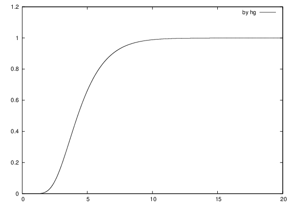
We first consider the case $m=5,n=7$ , $\Sigma^{-1}/2=\beta=(1,2,3,4,5)$ . For $x=20$ , the two bounds in (33) are given as $0.9996034$ and $0.9999987$ . With the initial value of $x_{0}=0.01$ and step size $0.0001$ we obtained

\Pr[\ell_{1}<20]=0.999972.

The cumulative distribution function for this case is plotted on the left part of Figure 2.

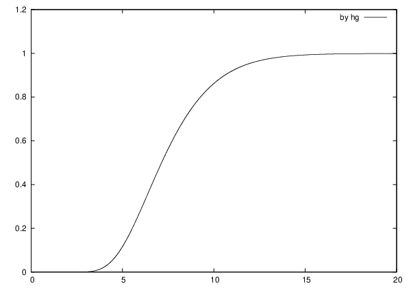
Next we consider the case $m=10,n=12$ , $\beta=(1,2,\dots,10)$ . For $x=30$ , the bounds are $(0.99866943,0.99999998)$ . For generation of initial values it takes about 20 seconds for approximating ${}_{1}\kern-0.50003ptF_{1}$ and its derivatives up to the degree 20 with an Intel Core i7 CPU. With the initial value of $x_{0}=0.2$ and step size 0.001, we obtain

\Pr[\ell_{1}<30]=0.999545

in about 75 seconds. The cumulative distribution function for this case is plotted on the right part of Figure 2. We see that enough accuracy is obtained even for $m=10$ within practical amount of time.

The Laplace approximation fails to give a probability for the above two cases too as in $m=2$ (see Section 3.1); it exceeds one.

The complexity of numerically solving the ODE for $\vec{G}$ (30) is

O(m2^{m})\times\mbox{(steps of the Runge-Kutta method with a prescribed precision)}.

In fact, since the matrix $P_{i}(\beta x)$ has sparsity, each vector $P_{i}(\beta x)\vec{G}(x)$ , which has $2^{m}$ elements, can be evaluated in $O(2^{m})$ steps at $x$ from the values of $\vec{G}(x)$ by utilizing (28).

7 Discussion of open problems

The holonomic gradient method ([23]) gives a general algorithm for obtaining the partial differential equations satisfied by parametrized definite integrals such as the normalizing constant of a family of probability distributions. In fact, in Nakayama et al. [23] and Sei et al. [28] we used the holonomic gradient method for deriving the partial differential equations of the normalizing constants and for maximum likelihood estimation for distributions in directional statistics. For the case of ${}_{1}\kern-0.50003ptF_{1}$ , the partial differential equations were already derived by Muirhead [20] more than 40 years ago. Our use of those partial differential equations for numerical evaluation of ${}_{1}\kern-0.50003ptF_{1}$ is very straightforward as discussed in Section 3 for the two dimensional case. Yet, from the viewpoint of holonomic functions, the partial differential equations of Muirhead [20] present many interesting open problems.

One important question is to obtain the ordinary and partial differential equations for the diagonal case as discussed in Section 3.2 for the case of $m=2$ . For a general dimension $m>2$ , it is desirable to be able to handle various patterns of diagonalization, such as the two-block diagonalization $y_{1}=\dots=y_{l}>y_{l+1}=\dots=y_{m}$ . A direct “by hand” calculation using the l’Hôpital rule becomes quickly infeasible when we increase $m$ . Also the use of the restriction algorithm for holonomic ideals is limited by computational complexity. It is in fact a very heavy algorithm. Currently the nk_restriction routine of Risa/Asir in Section 5.2 takes too much time for $m\geq 4$ . One possibility is to follow the approach in Muirhead [20] and Sugiyama et al. [33], where differentiation with respect to elementary symmetric functions of the roots of $Y$ are considered. As discussed in Section 5.2, we conjecture that the ideal $I$ generated by $\prod_{j\neq i}(y_{i}-y_{j})g_{i}$ , $i=1,\ldots,m$ in the Weyl algebra $D_{m}$ is an holonomic ideal. Holonomicity guarantees the existence of partial differential equations for diagonal regions.

Another question is to consider the asymptotics for $\Pr[\ell_{1}\geq x]=1-\Pr[\ell_{1}<x]$ as $x\rightarrow\infty$ . As mentioned in the previous section, this tail probability can be approximated by the tube method ([15], [16]). One theoretical problem in applying the tube method is that only the approximation for the tail probability itself has been justified and the justification of its derivatives has to be proved. However it is obvious that the current approach of taking the initial values close to the origin causes difficulty in precision for the extreme upper tail probability, in the case we want to evaluate the small probability $\Pr[\ell_{1}\geq x]$ . Hence it is desirable to be able to use tube formula approximation as the initial values at $x=\infty$ .

From computational viewpoint, our holonomic gradient method has exponential complexity in the dimension $m$ . We need to keep the $2^{m}$ -dimensional numerical vector $\vec{F}$ in memory at each step of the iteration. For $m=20$ , the dimension of the vector is about one million. Hence we do not expect that the current implementation of the holonomic gradient method works for $m=20$ . It might be possible to improve our current implementation by fully exploiting the fact that ${}_{1}\kern-0.50003ptF_{1}$ is a symmetric function in $Y$ .

Appendix A Holonomicity for dimension two

In the theory of holonomic functions, the holonomicity of the left ideal generated by the set of partial differential operators is an important question. In fact, the existence of the ordinary differential equation with polynomial coefficients for the function restricted to the diagonal region follows from the holonomicity. Holonomicity of the ideal generated by $g_{1},g_{2}$ in the two-dimensional case can be verified by Gröbner basis computation. Here we present this result. As to a general introduction to holonomic ideals and Gröbner bases, we refer to the Chapter 1 of Saito et al. [27].

Note that the holonomicity on the non-diagonal region ${\cal X}$ follows from Theorem 2 because the zero set of $y_{i}\xi_{i}^{2}=0$ , $i=1,\ldots,m$ contains the characteristic variety on ${\cal X}$ . The holonomicity on ${\cal X}$ can also be proved by an analogous method with Ibukiyama et al. [9].

Let $D_{2}$ be the second Weyl algebra. For $P=\sum_{k=0}^{d}\sum_{\alpha_{1}+\alpha_{2}=k}f_{\alpha_{1},\alpha_{2}}(y_{1},y_{2})\partial_{1}^{\alpha_{1}}\partial_{2}^{\alpha_{2}}\in D_{2},$ we define $\operatorname{in}(P)$ by

\displaystyle\operatorname{in}(P)=\sum_{\alpha_{1}+\alpha_{2}=d}f_{\alpha_{1},\alpha_{2}}(y_{1},y_{2})\xi_{1}^{\alpha_{1}}\xi_{2}^{\alpha_{2}}\in\mathbb{C}[y_{1},y_{2},\xi_{1},\xi_{2}],

where we assume that $f_{\alpha_{1},\alpha_{2}}(y_{1},y_{2})\in\mathbb{C}[y_{1},y_{2}]$ and that $f_{\alpha_{1},\alpha_{2}}(y_{1},y_{2})\neq 0$ for some $\alpha_{1},\alpha_{2}$ with $\alpha_{1}+\alpha_{2}=d$ . For a left ideal $I$ of $D_{2}$ , the characteristic variety $\operatorname{ch}(I)$ is defined by

\displaystyle\operatorname{ch}(I)=\{(y_{1},y_{2},\xi_{1},\xi_{2})\in\mathbb{C}^{2\cdot 2}\mid\forall P\in I,\operatorname{in}(P)(y_{1},y_{2},\xi_{1},\xi_{2})=0\}.

It is a basic fact that the dimension of the characteristic variety $\operatorname{ch}(I)$ of the proper left ideal $I$ of $D_{2}$ is greater than or equal to $2$ . A left ideal $I$ of $D_{2}$ is called holonomic if the dimension of the characteristic variety $\operatorname{ch}(I)$ equals $2$ .

Let $P_{1}=(y_{1}-y_{2})g_{1},P_{2}=(y_{2}-y_{1})g_{2}$ and let $I$ be the ideal of $D_{2}$ generated by $P_{1}$ and $P_{2}$ . We will show that $I$ is holonomic. Let $S=y_{2}\partial_{2}^{2}P_{1}+y_{1}\partial_{1}^{2}P_{2}+c(\partial_{2}P_{1}+\partial_{1}P_{2})\in I$ . By direct calculation we have

	$\displaystyle S=$	$\displaystyle(y_{1}^{2}y_{2}-y_{1}y_{2}^{2}+\frac{y_{1}^{2}}{2}-2y_{1}y_{2})\partial_{1}^{2}\partial_{2}+(-y_{1}^{2}y_{2}+y_{1}y_{2}^{2}-2y_{1}y_{2}+\frac{y_{2}^{2}}{2})\partial_{1}\partial_{2}^{2}-\frac{y_{1}^{2}}{2}\partial_{1}^{3}-\frac{y_{2}^{2}}{2}\partial_{2}^{3}$
		$\displaystyle+(ay_{1}^{2}-ay_{1}y_{2}-\frac{3cy_{1}}{2}-y_{1})\partial_{1}^{2}+(-y_{2}+2ay_{2}-ay_{1}y_{2}+ay_{2}^{2}-\frac{3cy_{2}}{2})\partial_{2}^{2}$
		$\displaystyle+(-cy_{1}^{2}+2cy_{1}y_{2}-cy_{2}^{2}+4y_{1}y_{2}-\frac{3cy_{1}}{2}-\frac{3cy_{2}}{2}+y_{1}+y_{2})\partial_{1}\partial_{2}$
		$\displaystyle+(acy_{1}-acy_{2}+2ay_{1}+cy_{1}-c^{2})\partial_{1}+(-c^{2}-acy_{1}+acy_{2}+cy_{2})\partial_{2}+2ac.$

Hence

\displaystyle\operatorname{in}(S)=

\displaystyle(y_{1}^{2}y_{2}-y_{1}y_{2}^{2}+\frac{y_{1}^{2}}{2}-2y_{1}y_{2})\xi_{1}^{2}\xi_{2}+(-y_{1}^{2}y_{2}+y_{1}y_{2}^{2}-2y_{1}y_{2}+\frac{y_{2}^{2}}{2})\xi_{1}\xi_{2}^{2}-\frac{y_{1}^{2}}{2}\xi_{1}^{3}-\frac{y_{2}^{2}}{2}\xi_{2}^{3}.

Consider the ideal $J$ of $\mathbb{C}[y_{1},y_{2},\xi_{1},\xi_{2}]$ generated by $\operatorname{in}(P_{1})$ , $\operatorname{in}(P_{2})$ and $\operatorname{in}(S)$ . The following is a Gröbner base of $J$ with respect to the graded reverse lexicographic order with $y_{1}>y_{2}>\xi_{1}>\xi_{2}$ :

	$\displaystyle\{y_{2}^{2}\xi_{1}^{3}\xi_{2}^{2}+3y_{2}^{2}\xi_{1}^{2}\xi_{2}^{3}+3y_{2}^{2}\xi_{1}\xi_{2}^{4}+y_{2}^{2}\xi_{2}^{5},y_{1}y_{2}\xi_{1}^{3}+3y_{1}y_{2}\xi_{1}^{2}\xi_{2}+3y_{2}^{2}\xi_{1}\xi_{2}^{2}+y_{2}^{2}\xi_{2}^{3},$
	$\displaystyle y_{1}^{2}\xi_{1}^{2}-y_{1}y_{2}\xi_{1}^{2},y_{1}y_{2}\xi_{2}^{2}-y_{2}^{2}\xi_{2}^{2}\}.$

Thus the Krull dimension of $J$ is $2$ . Since $\{P_{1},P_{2},S\}\subset I$ , the characteristic variety $\operatorname{ch}(I)$ of $I$ is contained in the zero set of $J$ . This implies that the dimension of $\operatorname{ch}(I)$ does not exceed $2$ and hence the dimension of $\operatorname{ch}(I)$ is equal to $2$ . Therefore $I$ is holonomic for $m=2$ .

Appendix B R source program for dimension two

The following program in data analysis system R implements holonomic gradient method for $m=2$ of Section 3.1 based on deSolve add-on package for R.

library(deSolve)
m <- 2    # dimension
n <- 3    # degrees of freedom
x <- 4.31600  #  specify x.   We evaluate  Pr( l1 < x )
b1 <- 1; b2 <- 2 #  (b1,b2) =  (1/2) diag(Sigma^{-1})
a <- (m+1)/2; c <- (n+m+1)/2;  totalsteps <- 10000; stepsize <- x/totalsteps

# h’s
h2000 <- function(y1,y2) a/y1
h2010 <- function(y1,y2) -(c-y1)/y1 - y2/(2*y1*(y1-y2))
h2001 <- function(y1,y2) y2/(2*y1*(y1-y2))
h1200 <- function(y1,y2) a/(2*y2*(y2-y1))
h1210 <- function(y1,y2) 3/(4*(y2-y1)^2) + a/y2 - (c-y1)/(2*y2*(y2-y1))
h1201 <- function(y1,y2) -3/(4*(y2-y1)^2)
h1211 <- function(y1,y2) -(c-y2)/y2 - y1/(2*y2*(y2-y1))

#initial values
x1 <- b1*stepsize; x2 <- b2*stepsize
fi <- c(a/c, (a*(a+1))/(c*(c+1)), (a*(a+1))/(3*c*(c+1)) + (2*a*(a-1/2))/(3*c*(c-1/2)),
       (a*(a+1)*(a+2))/(5*c*(c+1)*(c+2)) + (4*a*(a+1)*(a-1/2))/(5*c*(c+1)*(c-2/1)))
fi <- c(1+(x1+x2)*fi[1], fi[1]+x1*fi[2]+x2*fi[3], fi[1]+x2*fi[2]+x1*fi[3], fi[3]+(x1+x2)*fi[4])

# gradient
f11m2 <- function(y,fv,parm){y1 <- y*b1; y2 <- y*b2;
      list(c(
        b1*fv[2] + b2*fv[3],
        b1*(fv[1]*h2000(y1,y2)+fv[2]*h2010(y1,y2)+fv[3]*h2001(y1,y2)) + b2*fv[4],
       Ψb2*(fv[1]*h2000(y2,y1)+fv[2]*h2001(y2,y1)+fv[3]*h2010(y2,y1)) + b1*fv[4],
         b1*(fv[1]*h1200(y2,y1)+fv[2]*h1201(y2,y1)+fv[3]*h1210(y2,y1)+fv[4]*h1211(y2,y1))
        +b2*(fv[1]*h1200(y1,y2)+fv[2]*h1210(y1,y2)+fv[3]*h1201(y1,y2)+fv[4]*h1211(y1,y2)))
)}

output <- ode(fi,func=f11m2,(1:totalsteps)*x/totalsteps)
prob0 <- ((b1*b2)^(n/2)*gamma(a)*gamma(a-1/2))/(gamma(c)*gamma(c-1/2)) * x^(n*m/2) * exp(-x*(b1+b2))
cat("x=",x, "prob=", output[totalsteps,2]*prob0,"\n")

References

[1] Uri M. Ascher and Linda R. Petzold. Computer Methods for Ordinary Differential Equations and Differential-Algebraic Equations. Society for Industrial and Applied Mathematics (SIAM), Philadelphia, PA, 1998. ISBN 0-89871-412-5.
[2] Ronald Butler and Robert Paige. Exact distributional computations for Roy’s statistic and the largest eigenvalue of a Wishart distribution. Statistics and Computing, 21:147–157, 2011. ISSN 0960-3174.
[3] Ronald W. Butler and Andrew T. A. Wood. Laplace approximations for hypergeometric functions with matrix argument. Ann. Statist., 30(4):1155–1177, 2002. ISSN 0090-5364.
[4] A. G. Constantine. Some non-central distribution problems in multivariate analysis. Ann. Math. Statist., 34:1270–1285, 1963. ISSN 0003-4851.
[5] Kenneth I. Gross and Donald St. P. Richards. Special functions of matrix argument. I. Algebraic induction, zonal polynomials, and hypergeometric functions. Trans. Amer. Math. Soc., 301(2):781–811, 1987. ISSN 0002-9947.
[6] R. D. Gupta and D. St. P. Richards. Hypergeometric functions of scalar matrix argument are expressible in terms of classical hypergeometric functions. SIAM J. Math. Anal., 16:852–858, 1985. ISSN 1095-7154.
[7] Hiroki Hashiguchi and Naoto Niki. Numerical computation on distributions of the largest and the smallest latent roots of the Wishart matrix. J. Japanese Soc. Comput. Statist., 19(1):45–56, 2006. ISSN 0915-2350.
[8] Carl S. Herz. Bessel functions of matrix argument. Ann. of Math. (2), 61:474–523, 1955. ISSN 0003-486X.
[9] Tomoyoshi Ibukiyama, Takako Kuzumaki, and Hiroyuki Ochiai. Holonomic systems of Gegenbauer type polynomials of matrix arguments related with Siegel modular forms. Journal of the Mathematical Society of Japan. In Press.
[10] Alan T. James. Distributions of matrix variates and latent roots derived from normal samples. Ann. Math. Statist., 35:475–501, 1964. ISSN 0003-4851.
[11] Alan T. James. Calculation of zonal polynomial coefficients by use of the Laplace-Beltrami operator. Ann. Math. Statist, 39:1711–1718, 1968. ISSN 0003-4851.
[12] I.M. Johnstone. On the distribution of the largest eigenvalue in principal components analysis. The Annals of statistics, 29(2):295–327, 2001.
[13] I.M. Johnstone. Multivariate analysis and jacobi ensembles: Largest eigenvalue, tracy–widom limits and rates of convergence. The Annals of statistics, 36(6):2638–2716, 2008.
[14] Plamen Koev and Alan Edelman. The efficient evaluation of the hypergeometric function of a matrix argument. Math. Comp., 75(254):833–846, 2006. ISSN 0025-5718.
[15] Satoshi Kuriki and Akimichi Takemura. Tail probabilities of the maxima of multilinear forms and their applications. Ann. Statist., 29(2):328–371, 2001. ISSN 0090-5364.
[16] Satoshi Kuriki and Akimichi Takemura. Euler characteristic heuristic for approximating the distribution of the largest eigenvalue of an orthogonally invariant random matrix. J. Statist. Plann. Inference, 138(11):3357–3378, 2008. ISSN 0378-3758.
[17] Vadim B. Kuznetsov and Siddhartha Sahi, editors. Jack, Hall-Littlewood and Macdonald Polynomials, volume 417 of Contemporary Mathematics, Providence, RI, 2006. American Mathematical Society. ISBN 0-8218-3683-8.
[18] I. G. Macdonald. Symmetric Functions and Hall Polynomials. Oxford Mathematical Monographs. The Clarendon Press Oxford University Press, New York, second edition, 1995. ISBN 0-19-853489-2. With contributions by A. Zelevinsky, Oxford Science Publications.
[19] A. M. Mathai, Serge B. Provost, and Takesi Hayakawa. Bilinear Forms and Zonal Polynomials, volume 102 of Lecture Notes in Statistics. Springer-Verlag, New York, 1995. ISBN 0-387-94522-9.
[20] R. J. Muirhead. Systems of partial differential equations for hypergeometric functions of matrix argument. Ann. Math. Statist., 41:991–1001, 1970. ISSN 0003-4851.
[21] Robb J. Muirhead. Latent roots and matrix variates: a review of some asymptotic results. Ann. Statist., 6(1):5–33, 1978. ISSN 0090-5364.
[22] Robb J. Muirhead. Aspects of Multivariate Statistical Theory. John Wiley & Sons Inc., New York, 1982. ISBN 0-471-09442-0. Wiley Series in Probability and Mathematical Statistics.
[23] Hiromasa Nakayama, Kenta Nishiyama, Masayuki Noro, Katsuyoshi Ohara, Tomonari Sei, Nobuki Takayama, and Akimichi Takemura. Holonomic gradient descent and its application to the Fisher-Bingham integral. Advances in Applied Mathematics, 47:639–658, 2011. ISSN 0196-8858.
[24] Toshinori Oaku. Algorithms for $b$ -functions, restrictions, and algebraic local cohomology groups of $D$ -modules. Adv. in Appl. Math., 19(1):61–105, 1997. ISSN 0196-8858.
[25] D. St. P. Richards. Functions of matrix argument. In NIST Handbook of Mathematical Functions, pages 767–774. U.S. Dept. Commerce, Washington, DC, 2010.
[26] RisaAsir developing team. Risa/asir, a computer algebra system. Available at http://www.math.kobe-u.ac.jp/Asir/.
[27] Mutsumi Saito, Bernd Sturmfels, and Nobuki Takayama. Gröbner Deformations of Hypergeometric Differential Equations, volume 6 of Algorithms and Computation in Mathematics. Springer-Verlag, Berlin, 2000. ISBN 3-540-66065-8.
[28] Tomonari Sei, Hiroki Shibata, Akimichi Takemura, Katsuyoshi Ohara, and Nobuki Takayama. Properties and applications of Fisher distribution on the rotation group, 2011. arXiv:1110.0721v1.
[29] Richard P. Stanley. Some combinatorial properties of Jack symmetric functions. Adv. Math., 77(1):76–115, 1989. ISSN 0001-8708.
[30] W. A. Stein et al. Sage Mathematics Software (Version 4.7.2). The Sage Development Team, 2011. http://www.sagemath.org.
[31] Takakazu Sugiyama. On the distribution of the largest latent root of the covariance matrix. Ann. Math. Statist, 38:1148–1151, 1967. ISSN 0003-4851.
[32] Takakazu Sugiyama. Approximation for the distribution of the largest latent root of a Wishart matrix. Austral. J. Statist., 14:17–24, 1972. ISSN 0004-9581.
[33] Takakazu Sugiyama, Yuuichi Takeda, and Masafumi Fukuda. On the numerical computation of confluent hypergeometric function with zonal polynomials of order 3. J. Japanese Soc. Computat. Statist., 11(1):1–8, 1998. ISSN 0915-2350.
[34] Akimichi Takemura. Zonal Polynomials. Institute of Mathematical Statistics Lecture Notes—Monograph Series, 4. Institute of Mathematical Statistics, Hayward, CA, 1984. ISBN 0-940600-05-6.
[35] Akimichi Takemura and Yo Sheena. Distribution of eigenvalues and eigenvectors of Wishart matrix when the population eigenvalues are infinitely dispersed and its application to minimax estimation of covariance matrix. J. Multivariate Anal., 94(2):271–299, 2005. ISSN 0047-259X.
[36] Doron Zeilberger. A holonomic systems approach to special functions identities. J. Comput. Appl. Math., 32(3):321–368, 1990. ISSN 0377-0427.

	$\displaystyle\Pr[\ell_{1}<x\|\mathop{{\rm diag}}(\sigma_{1}^{2},\dots,\sigma_{1}^{2})]$	$\displaystyle\leq\Pr[\ell_{1}<x\|\mathop{{\rm diag}}(\sigma_{1}^{2},\dots,\sigma_{m}^{2})]$
		$\displaystyle\leq\Pr[\ell_{1}<x\|\mathop{{\rm diag}}(\sigma_{1}^{2},0,\dots,0)].$		(33)