跳到论文正文
W Papers独立论文阅读器 arXiv:1201.0320 论文正文 计算阅读时间 · 0%
引用这篇论文根据当前论文元数据生成,正式投稿前建议核对。


License: arXiv.org perpetual non-exclusive license
arXiv:1201.0320v2 [cs.IT] 20 Feb 2013

Optimal Distributed Resource Allocation for Decode-and-Forward Relay Networks

Yin Sun    Zhoujia Mao    Xiaofeng Zhong    Yuanzhang Xiao    Shidong Zhou    Ness B. Shroff ††thanks: Y. Sun and Z. Mao are with the Department of Electrical and Computer Engineering, the Ohio State University, 2015 Neil Ave., Columbus, OH 43210, USA. sunyin02@gmail.com, maoz@ece.osu.edu.††thanks: X. Zhong and S. Zhou are with the State Key Laboratory on Microwave and Digital Communications, Tsinghua National Laboratory for Information Science and Technology, and Department of Electronic Engineering, Tsinghua University, Beijing, China. Address: Room 4-407, FIT Building, Tsinghua University, Beijing 100084, People’s Republic of China. {zhongxf,zhousd}@tsinghua.edu.cn.††thanks: Y. Xiao is with the Department of Electrical Engineering, University of California, Los Angeles. e-mail: xyz.xiao@gmail.com.††thanks: N. B. Shroff is with the Department of Electrical and Computer Engineering and the Department of Computer Science and Engineering, the Ohio State University, 2015 Neil Ave., Columbus, OH 43210, USA. shroff@ece.osu.edu.††thanks: The material in this paper was presented in part in IEEE GLOBECOM 2009.
Abstract

This paper presents a distributed resource allocation algorithm to jointly optimize the power allocation, channel allocation and relay selection for decode-and-forward (DF) relay networks with a large number of sources, relays, and destinations. The well-known dual decomposition technique cannot directly be applied to resolve this problem, because the achievable data rate of DF relaying is not strictly concave, and thus the local resource allocation subproblem may have non-unique solutions. We resolve this non-strict concavity problem by using the idea of the proximal point method, which adds quadratic terms to make the objective function strictly concave. However, the proximal solution adds an extra layer of iterations over typical duality based approaches, which can significantly slow down the speed of convergence. To address this key weakness, we devise a fast algorithm without the need for this additional layer of iterations, which converges to the optimal solution. Our algorithm only needs local information exchange, and can easily adapt to variations of network size and topology. We prove that our distributed resource allocation algorithm converges to the optimal solution. A channel resource adjustment method is further developed to provide more channel resources to the bottleneck links and realize traffic load balance. Numerical results are provided to illustrate the benefits of our algorithm.
Index terms−- Decode-and-forward, distributed resource allocation, wireless relay network.

I Introduction

Cooperative relaying has recently received a lot of attention as a promising technique to improve the throughput, coverage, and reliability of wireless networks [1, 2]. The decode-and-forward (DF) relay strategy has been advocated by several standard organizations for next generation wireless networks [3, 4, 5]. In this strategy, a source node, a relay node, and a destination node cooperate to form a DF relay link. The relay node decodes the source node’s transmission message, then forwards the recovered message to the destination.

Since power and channel (code, time, and/or frequency) are crucial resources in wireless networks, a number of studies have investigated the resource allocation for DF relay networks. They have shown that optimal resource allocation can achieve significant performance improvement for DF relay networks with a single source-destination data stream [6, 7, 8, 9, 10, 11, 12, 13, 14, 15, 16]. However, optimal resource allocation becomes much more challenging in scenarios with many sources, relays, and destinations, because each source-destination data stream may cooperate with several relay nodes and each relay node can assist several data streams, which could form a large number of potential DF relay links. In order to achieve higher network throughput, appropriate DF relay links should be selected out and allocated with suitable source power, relay power, and channel resources for transmissions.

Fig. 1: A DF relay network with 3 source-destination data streams and 2 relays.

Centralized power allocation and relay selection algorithms of relay networks were proposed in [17, 18, 19, 20], which requests signaling mechanisms to gather the channel state information (CSI) of all the wireless links at a central control node. However, such mechanisms are difficult to implement in practice and will especially not work well when the network size is large. Recently, a great deal of research efforts have focused on distributed resource allocation for DF relay networks: Traditional two-hop relaying was considered in [21, 22, 23], which ignores the source-destination wireless channel, and thus achieves a lower data rate. In [24, 25, 26], several other conservative rate functions of DF relaying were employed to simplify the distributed resource allocation problem and make it tractable. Optimal power allocation of the relay nodes was studied in [17, 18, 27, 19, 20] without considering power allocation of the source node and relay selection. Optimal distributed resource allocation for DF relay networks remains to be a difficult and crucial problem.

Dual decomposition techniques have been effectively used in multi-hop wireless networks to achieve optimal resource allocation results (e.g., see [28] and the references therein). However, such techniques cannot be applied directly to DF relay networks —- the local resource allocation subproblems may have non-unique optimal solutions, because the achievable rate of DF relaying is not strictly concave. Since no global network information is available to the local resource allocation solvers, it is quite difficult to find a global feasible solution among all the locally optimal solutions [29, 30].

One promising method to address this non-strict concavity problem is the proximal point method [31], which adds strictly concave terms to the achievable rate function without affecting the optimal solution. However, typical proximal point algorithms require an extra outer layer of iterations compared to the conventional dual decomposition based algorithms [31], which, in turn, results in a slower convergence speed.

In this paper, we investigate the optimal resource allocation of DF relay networks, which may have a large number of sources, relays, and destinations. Each source node may transmit to one or several destinations through the assistance of several relay nodes. Meanwhile, each relay node may aid several source-destination data streams, as illustrated in Fig. 1. Each of the source and relay nodes has an individual transmission power constraint. The channel resources (code, time, and/or frequency) of the network are managed by many distributed control nodes. Each control node is pre-assigned with some channel resources, and is responsible to allocate these channel resources to nearby wireless links. The main contributions of this paper are summarized as follows:

  • •

    We propose a distributed resource allocation algorithm that jointly optimizes the power allocation, channel allocation and relay selection of DF relay networks so as to maximize the total throughput. The candidate DF relay links compete for the channel resources and the DF relay links with zero (or very few) channel resources are not selected for transmission. By this, the optimal relay selection is obtained through channel allocation. Our algorithm requires less layers of iterations than traditional proximal point algorithms, and thus have a much faster convergence speed. In addition, our algorithm only needs local information exchange among the source, relay, destination, and control nodes of each DF relay link, and can easily adapt to variations of network size and topology. We prove that this algorithm converges to the optimal resource allocation solution.

  • •

    In practice, the spatial distribution of wireless traffic is usually non-uniform and varies from time to time. The pre-assigned channel resources of the distributed control nodes may be inadequate to support the heavy wireless traffic. To address this problem, we develop a centralized channel resource adjustment algorithm on top of the proposed distributive resource allocation algorithm. The bottleneck control nodes are provided with more channel resources in order to balance the traffic load.

The proposed power allocation algorithm is motivated by the work in [32], where a modified proximal point algorithm with less iteration layers was proposed for multi-path routing problems. However, the structure of the objective function in that work is very different from our work that deals with DF relay networks. Hence, a substantially new proof methodology is required to show convergence in our context, which is one of the major contributions of this paper.

The remaining parts of this paper are organized as follows: In Section II, we present the system model and the formulation of power allocation problem. In Section III, we describe our distributed power allocation algorithm. A centralized channel resource adjustment algorithm is presented in Section IV. Some simple extensions of our algorithm are discussed in Section V. Numerical results are provided in Section VI, and we conclude the paper in Section VII.

II System Model and Problem Formulation

Consider a DF relay network with NN source/destination nodes, denoted by the set 𝒩={1,2,…,N}\mathcal{N}=\{1,2,\ldots,N\}, and JJ relay nodes, represented by the set 𝒥={1,2,…,J}\mathcal{J}=\{1,2,\ldots,J\}. Each source-destination data stream in the network is denoted as m=(s,d)m=(s,d) with s,d∈𝒩s,d\in\mathcal{N}. The set of all data streams is denoted by ℳ⊆{(i,j)|i,j∈𝒩,i≠j}\mathcal{M}\subseteq\{(i,j)|i,j\in\mathcal{N},i\neq j\}. The mmth data stream either can transmit directly through the source-destination wireless channel, or can be assisted by J⁡(m)J(m) candidate relay nodes and form J⁡(m)J(m) possible DF relay links. The set of candidate relay nodes for the mmth data stream is denoted by 𝒥⁡(m)⊆𝒥\mathcal{J}(m)\subseteq\mathcal{J}. We assume that each DF relay link only involves one relay node. When several relay nodes assist the same source-destination data stream, they belong to different DF relay links to avoid the implementation complexity due to the cooperation among different relay nodes. We further assume that the direct transmission (DT) link and DF relay links of each data stream operate over orthogonal wireless channels by means of code division multiple access (CDMA), or frequency/time division multiple access (F/TDMA) as in [27, 19].

The wireless transmissions in this network are managed by TT distributed control nodes, which are denoted by 𝒯={1,2,…,T}\mathcal{T}=\{1,2,\ldots,T\}. The candidate wireless links of data stream mm, including J⁡(m)J(m) DF relay links and one direct transmission (DT) link, are managed by the control node c⁡(m)c(m). We assume that neighboring control nodes are assigned to orthogonal channels to suppress co-channel interference, and distant control nodes are allowed to reuse the same channel resources. Such an assumption is practical for many wireless networks. For example, in wireless sensor networks, the traffic load and the transmission power are very small and hence interference is less of an issue [33, 34].

The DF relay procedure consists of two phases: In Phase 1, the source node transmits a message to the relay and destination nodes. The relay node decodes its received message, while the destination stores its received signal for later decoding. In Phase 2, the relay node forwards the recovered message to the destination. The destination combines its received signals in two phases to decode the source node’s message [2]. Let hms,dh_{m}^{s,d} denotes the complex channel coefficient of the source-destination wireless link of data stream mm, hm​js,rh_{mj}^{s,r} and hm​jr,dh_{mj}^{r,d} denote the complex channel coefficients of the source-relay and relay-destination links of the DF relay link composed by data stream mm and relay node jj.

The spectrum efficiency of the DT link of data stream mm is given by the capacity of Gaussian channel, i.e.,

RmD​T=θmD​T​log2⁡(+Pms​|hms,d|2θmD​T​N0​W)=θmD​T​log2⁡(+Pms​gms,dθmD​T),\displaystyle R_{m}^{DT}\!=\!\theta_{m}^{DT}\!\log_{2}\!\left(\!1\!+\!\frac{P^{s}_{m}|h^{s,d}_{m}|^{2}}{\theta_{m}^{DT}N_{0}W}\!\right)\!=\!\theta_{m}^{DT}\!\log_{2}\!\left(\!1\!+\!\frac{P^{s}_{m}g^{s,d}_{m}}{\theta_{m}^{DT}}\!\right)\!\!,\!\!\! (1)

where Pms≥0P^{s}_{m}\geq 0 is transmission power of the source node, θmD​T\theta_{m}^{DT} is the corresponding proportion of channel resources, WW is the total amount of available channel resources, N0N_{0} is power spectral density of the Gaussian noise at each receiver, and gms,d≜|hms,d|2N0​Wg_{m}^{s,d}\triangleq\frac{|h_{m}^{s,d}|^{2}}{N_{0}W} characterizes the quality of the source-destination wireless channel of the mmth data stream, as shown in Fig. 2. The spectrum efficiency achieved by the DF relay link composed by data stream mm and relay node jj can be described as [2]:

Rm​jD​F\displaystyle R_{mj}^{DF}\!\!\!\!\!\!\!\!\!\! =θm​jD​F2min{log2(1+2​Pm​js​|hm​js,r|2θm​jD​F​N0​W),\displaystyle=\frac{\theta_{mj}^{DF}}{2}\min\left\{\log_{2}\left(1+\frac{2P^{s}_{mj}|h^{s,r}_{mj}|^{2}}{\theta_{mj}^{DF}N_{0}W}\right),\right. (2)
log2[1+2​(Pm​js​|hms,d|2+Pm​jr​|hm​jr,d|2)θm​jD​F​N0​W]}\displaystyle~~~~~~~~~\left.\log_{2}\left[1+\frac{2\big(P^{s}_{mj}|h^{s,d}_{m}|^{2}+P^{r}_{mj}|h^{r,d}_{mj}|^{2}\big)}{\theta_{mj}^{DF}N_{0}W}\right]\right\}
=θm​jD​F2min{log2(1+2​Pm​js​gm​js,rθm​jD​F),\displaystyle=\frac{\theta_{mj}^{DF}}{2}\min\left\{\log_{2}\left(1+\frac{2P^{s}_{mj}g^{s,r}_{mj}}{\theta_{mj}^{DF}}\right),\right.
log2[1+2​(Pm​js​gms,d+Pm​jr​gm​jr,d)θm​jD​F]},\displaystyle~~~~~~~~~\left.\log_{2}\left[1+\frac{2\big(P^{s}_{mj}g^{s,d}_{m}+P^{r}_{mj}g^{r,d}_{mj}\big)}{\theta_{mj}^{DF}}\right]\right\},

where Pm​js,Pm​jr≥0P^{s}_{mj},P^{r}_{mj}\geq 0 are the transmission powers of the source and relay nodes, θm​jD​F\theta_{mj}^{DF} is the corresponding proportion of channel resources, gm​js,r≜|hm​js,r|2N0​Wg_{mj}^{s,r}\triangleq\frac{|h_{mj}^{s,r}|^{2}}{N_{0}W} and gm​jr,d≜|hm​jr,d|2N0​Wg_{mj}^{r,d}\triangleq\frac{|h_{mj}^{r,d}|^{2}}{N_{0}W} characterize the quality of the source-relay and relay-destination wireless channels of this DF relay link.

Refer to caption
Fig. 2: Illustration of the DF relay strategy.

Let s⁡(m)s(m) represent the source node of data stream mm. Then, the power constraint of source node ll over all the channels can be determined as

∑{m|s⁡(m)=l}(Pms+∑j∈𝒥⁡(m)Pm​js)≤Pl,maxs,\displaystyle\sum_{\{m|s(m)=l\}}\left(P^{s}_{m}+\sum_{j\in\mathcal{J}(m)}P^{s}_{mj}\right)\leq P^{s}_{l,\max},

where Pl,maxsP^{s}_{l,\max} is the maximal transmission power of source node ll. The power constraint of relay node jj is expressed as

∑{m|j∈𝒥⁡(m)}Pm​jr≤Pj,maxr,\displaystyle\sum_{\{m|j\in\mathcal{J}(m)\}}P^{r}_{mj}\leq P^{r}_{j,\max},

where Pj,maxrP^{r}_{j,\max} is the maximal transmission power of relay node jj. The local channel resource constraint managed by control node tt is given by

∑{m|c⁡(m)=t}(θmD​T+∑j∈𝒥⁡(m)θm​jD​F)≤βt,\displaystyle\sum_{\{m|c(m)=t\}}\left(\theta_{m}^{DT}+\sum_{j\in\mathcal{J}(m)}\theta_{mj}^{DF}\right)\leq\beta_{t},

where βt\beta_{t} represent the proportion of channel resources pre-assigned to control node tt.

In practice, the channel codes with short block length usually have quite poor error performance [35]. The code block length and corresponding occupied channel resources should be large enough to guarantee a small decoding error probability, and the links with very few channel resources are not admitted for transmission. This requirement can be expressed by the following channel resource constraint:

θmD​T,θm​jD​F≥θmin,\displaystyle\theta_{m}^{DT},\theta_{mj}^{DF}\geq\theta_{\min}, (3)

where θmin>0\theta_{\min}>0 is a very small constant. If the channel resource fraction of a DF relay link or a DT link is equal to θmin\theta_{\min}, the network will not admit the transmission of this link. In such a way, the optimal relay selection is fulfilled. From the perspective of optimization, setting the minimum value θmin\theta_{\min} can avoid the channel resources from approaching zero, and thus preventing unnecessary technical complications due to non-differentiable achievable rates RmD​TR_{m}^{DT} and Rm​jD​FR_{mj}^{DF}.

The joint design of power allocation, channel allocation, and relay selection of the DF relay network is formulated as

(P)​maxPms,Pm​js,Pm​jr,θmD​T,θm​jD​F\displaystyle\!\!\!\!(\textrm{P})\max\limits_{\begin{subarray}{c}P^{s}_{m},P^{s}_{mj},P^{r}_{mj},\theta_{m}^{DT},\theta_{mj}^{DF}\end{subarray}} ∑m=1M(RmD​T+∑j∈𝒥⁡(m)Rm​jD​F)\displaystyle\sum_{m=1}^{M}\left(R_{m}^{DT}+\sum_{j\in\mathcal{J}(m)}R_{mj}^{DF}\right) (4a)
s.t.\displaystyle\rm{s.t.}~~~~~ ∑{m|s⁡(m)=l}(Pms+∑j∈𝒥⁡(m)Pm​js)≤Pl,maxs,∀l\displaystyle\!\!\!\!\!\!\!\!\sum_{\{m|s(m)=l\}}\left(P^{s}_{m}+\sum_{j\in\mathcal{J}(m)}\!\!P^{s}_{mj}\right)\!\leq\!P^{s}_{l,\max},\forall~l\!\! (4b)
∑{m|j∈𝒥⁡(m)}Pm​jr≤Pj,maxr,∀j\displaystyle\!\!\!\!\!\!\!\!\sum_{\{m|j\in\mathcal{J}(m)\}}P^{r}_{mj}\leq P^{r}_{j,\max},\forall~j (4c)
∑{m|c⁡(m)=t}(θmD​T+∑j∈𝒥⁡(m)θm​jD​F)≤βt,∀t\displaystyle\!\!\!\!\!\!\!\!\sum_{\{m|c(m)=t\}}\left(\theta_{m}^{DT}+\sum_{j\in\mathcal{J}(m)}\theta_{mj}^{DF}\right)\leq\beta_{t},~\forall~t (4d)
Pms,Pm​js,Pm​jr≥0,∀m,j,\displaystyle P^{s}_{m},P^{s}_{mj},P^{r}_{mj}\geq 0,\forall~m,j, (4e)
θmD​T,θm​jD​F≥θmin,∀m,j.\displaystyle\theta_{m}^{DT},\theta_{mj}^{DF}\geq\theta_{\min},\forall~m,j. (4f)

Note that although all the candidate DT and DF relay links are included in the objective function of Problem (P)(P), only the wireless links with channel resources larger than θmin\theta_{\min} are admitted for transmission after solving Problem (P)(P). If gm​js,r≤gms,dg_{mj}^{s,r}\leq g_{m}^{s,d}, one can simply show that Rm​jD​F<RmD​TR_{mj}^{DF}<R_{m}^{DT}. Hence, DF relaying cannot achieve a higher data rate than DT transmission in this case. Therefore, only the relay nodes satisfying gm​js,r>gms,dg_{mj}^{s,r}>g_{m}^{s,d} need to be considered in the candidate relay set 𝒥⁡(m)\mathcal{J}(m) for date stream mm.

The achievable rates RmD​TR_{m}^{DT} and Rm​jD​FR_{mj}^{DF} are both concave in their power and channel resource variables. Therefore, the resource allocation problem (P)(\textrm{P}) is a convex optimization problem. However, as we have mentioned earlier, the achievable rate of DF relaying Rm​jD​FR_{mj}^{DF} is not strictly concave. Specifically, Rm​jD​FR_{mj}^{DF} is linear in the transmission power variables Pm​jsP^{s}_{mj} and Pm​jrP^{r}_{mj} in two cases: When Pm​js​gm​js,r<Pm​js​gms,d+Pm​jr​gm​jr,dP^{s}_{mj}g^{s,r}_{mj}<P^{s}_{mj}g^{s,d}_{m}+P^{r}_{mj}g^{r,d}_{mj} holds, the achievable rate Rm​jD​FR_{mj}^{DF} in (2) does not vary with respect to Pm​jrP^{r}_{mj}. Moreover, if Pm​js​gm​js,r>Pm​js​gms,d+Pm​jr​gm​jr,dP^{s}_{mj}g^{s,r}_{mj}>P^{s}_{mj}g^{s,d}_{m}+P^{r}_{mj}g^{r,d}_{mj} holds and the value of Pm​js​gms,d+Pm​jr​gm​jr,dP^{s}_{mj}g^{s,d}_{m}+P^{r}_{mj}g^{r,d}_{mj} is fixed, Rm​jD​FR_{mj}^{DF} maintains the same value as Pm​jrP^{r}_{mj} varies.

In dual decomposition based distributed optimization techniques, it is quite difficult to recover the optimal primal variables (i.e., the transmission power variables Pm​jsP^{s}_{mj} and Pm​jrP^{r}_{mj}), if the objective function is non-strictly concave [36, 29, 30, 24]. Although the dual variables converge to the optimal solution to the dual problem, the primal variables may oscillate forever and never result in a feasible solution [32]. In the next section, we develop a distributed power allocation algorithm to address this non-strict concavity difficulty, and then prove its convergence to the optimal solution.

III Distributed Resource Allocation

To circumvent this non-strict concavity difficulty, we use the idea of proximal point method [31], which is to add some quadratic terms and make the objective function strictly concave in the primal variables. However, a standard proximal point method is not effective because it relies on an extra outer layer of iterations, and hence results in a slow convergence speed. We will overcome this difficulty by developing a distributed resource allocation algorithm without increasing the number of iteration layers. The details are provided below.

III-A Distributed Resource Allocation Algorithm

The original problem (P)(\textrm{P}) is rewritten as the following problem with some extra auxiliary variables:

max⁡∑m=1MPms,Pm​js,Pm​jr,θmD​T,θm​jD​FQms,Qm​js,Qm​jr⁡[RmD​T−cm2​(Pms−Qms)2]\displaystyle\!\!\!\!\!\!\!\!\!\!\!\!\!\!\!\!\!\!\!\!\!\!\!\!\!\!\!\max\limits_{\begin{subarray}{c}P^{s}_{m},P^{s}_{mj},P^{r}_{mj},\theta_{m}^{DT},\theta_{mj}^{DF}\\ Q^{s}_{m},Q^{s}_{mj},Q^{r}_{mj}\end{subarray}}~~\sum_{m=1}^{M}\left[R_{m}^{DT}-\frac{c_{m}}{2}\left(P^{s}_{m}-Q^{s}_{m}\right)^{2}\right]
+∑m=1M∑j∈𝒥⁡(m)[Rm​jD​F−cm​j2(Pm​js−Qm​js)2\displaystyle~+\sum_{m=1}^{M}\sum_{j\in\mathcal{J}(m)}\left[R_{mj}^{DF}-\frac{c_{mj}}{2}\left(P^{s}_{mj}-Q^{s}_{mj}\right)^{2}\right.
−cm​j2(Pm​jr−Qm​jr)2]\displaystyle~~~~~~~~~~~~~~~~~~~~~~~~~\left.-\frac{c_{mj}}{2}\left(P^{r}_{mj}-Q^{r}_{mj}\right)^{2}\right] (5a)
s.t.\displaystyle~~~~~~~\rm{s.t.} ∑{m|s⁡(m)=l}(Pms+∑j∈𝒥⁡(m)Pm​js)≤Pl,maxs,∀l\displaystyle\sum_{\{m|s(m)=l\}}\left(P^{s}_{m}+\sum_{j\in\mathcal{J}(m)}P^{s}_{mj}\right)\!\leq\!P^{s}_{l,\max},\forall~l\!\! (5b)
∑{m|j∈𝒥⁡(m)}Pm​jr≤Pj,maxr,∀j\displaystyle\sum_{\{m|j\in\mathcal{J}(m)\}}P^{r}_{mj}\leq P^{r}_{j,\max},\forall~j (5c)
∑{m|c⁡(m)=t}(θmD​T+∑j∈𝒥⁡(m)θm​jD​F)≤βt,∀t\displaystyle\sum_{\{m|c(m)=t\}}\left(\theta_{m}^{DT}+\sum_{j\in\mathcal{J}(m)}\theta_{mj}^{DF}\right)\leq\beta_{t},~\forall~t (5d)
Pms,Pm​js,Pm​jr≥0,∀m,j,\displaystyle~~~~P^{s}_{m},P^{s}_{mj},P^{r}_{mj}\geq 0,\forall~m,j, (5e)
θmD​T,θm​jD​F≥θmin,∀m,j,\displaystyle~~~~\theta_{m}^{DT},\theta_{mj}^{DF}\geq\theta_{\min},\forall~m,j, (5f)

where cm,cm​j>0c_{m},c_{mj}>0 are algorithm parameters, QmsQ^{s}_{m}, Qm​jsQ^{s}_{mj}, and Qm​jrQ^{r}_{mj} are auxiliary variables corresponding to PmsP^{s}_{m}, Pm​jsP^{s}_{mj}, and Pm​jrP^{r}_{mj}, respectively. It is easy to show that the optimal value of (5a) coincides with that of (4a) [31]. In fact, let P→⋆\vec{P}^{\star} denote the maximizer of (P)(\textrm{P}), then P→=P→⋆\vec{P}=\vec{P}^{\star}, Q→=P→⋆\vec{Q}=\vec{P}^{\star} maximizes (5). Moreover, problem (5) is strictly concave with respect to the transmission power variables PmsP^{s}_{m}, Pm​jsP^{s}_{mj}, and Pm​jrP^{r}_{mj}. In the sequent, we solve problem (5) instead of the original problem (P)(\textrm{P}).

Let μl\mu_{l} and νj\nu_{j} be the Lagrange multipliers associated with the constraints in (5b) and (5c), respectively. The partial Lagrangian of problem (5) with respect to the power constraints (5b) and (5c) is given by

L⁡(Pms,Pm​js,Pm​jr,Qms,Qm​js,Qm​jr,θmD​T,θm​jD​F,μl,νj)\displaystyle L\left(P^{s}_{m},P^{s}_{mj},P^{r}_{mj},Q^{s}_{m},Q^{s}_{mj},Q^{r}_{mj},\theta_{m}^{DT},\theta_{mj}^{DF};\mu_{l},\nu_{j}\right)
=\displaystyle= ∑m=1M{[RmD​T−cm2(Pms−Qms)2]\displaystyle\sum_{m=1}^{M}\bigg\{\left[R_{m}^{DT}-\frac{c_{m}}{2}\left(P^{s}_{m}-Q^{s}_{m}\right)^{2}\right]
+∑j∈𝒥⁡(m)[Rm​jD​F−cm​j2(Pm​js−Qm​js)2\displaystyle+\sum_{j\in\mathcal{J}(m)}\left[R_{mj}^{DF}-\frac{c_{mj}}{2}\left(P^{s}_{mj}-Q^{s}_{mj}\right)^{2}\right.
−cm​j2(Pm​jr−Qm​jr)2]}\displaystyle\left.~~~~~~~~~~~~~~~~~~-\frac{c_{mj}}{2}\left(P^{r}_{mj}-Q^{r}_{mj}\right)^{2}\right]\bigg\}
−∑l=1Nμl[∑{m|s⁡(m)=l}(Pms+∑j∈𝒥⁡(m)Pm​js−Pl,maxs)]\displaystyle-\sum_{l=1}^{N}\mu_{l}\left[\sum_{\{m|s(m)=l\}}\left(P^{s}_{m}+\sum_{j\in\mathcal{J}(m)}P^{s}_{mj}-P^{s}_{l,\max}\right)\right]
−∑j=1Jνj(∑{m|j∈𝒥⁡(m)}Pm​jr−Pj,maxr).\displaystyle-\sum_{j=1}^{J}\nu_{j}\left(\sum_{\{m|j\in\mathcal{J}(m)\}}P^{r}_{mj}-P^{r}_{j,\max}\right). (6)

For convenience, we rearrange the above Lagrangian as

L⁡(P→,Q→,θ→,ν→)\displaystyle L\left(\vec{P},\vec{Q},\vec{\theta};\vec{\nu}\right)
=\displaystyle= R⁡(P→,θ→)−12​(P→−Q→)T​V​(P→−Q→)−ν→T​(E​P→−P→max),\displaystyle R\left(\vec{P},\vec{\theta}\right)\!-\!\frac{1}{2}\left(\vec{P}\!-\!\vec{Q}\right)^{T}V\left(\vec{P}\!-\!\vec{Q}\right)\!-\!\vec{\nu}^{T}\left(E\vec{P}\!-\!\vec{P}_{\max}\right),\!\!\! (7)

where R⁡(P→,θ→)R(\vec{P},\vec{\theta}) is the objective function of problem (P)(\textrm{P}), θ→\vec{\theta} is a M+∑m=1MJ⁡(m)M+\sum_{m=1}^{M}J(m) dimensional vector representing the channel resources of the DT and DF relay links θmD​T\theta_{m}^{DT} and θm​jD​F\theta_{mj}^{DF}, P→\vec{P} is a M+2​∑m=1MJ⁡(m)M+2\sum_{m=1}^{M}J(m) dimensional vector representing the power allocation variables PmsP^{s}_{m}, Pm​jsP^{s}_{mj}, and Pm​jrP^{r}_{mj}, Q→\vec{Q} is a M+2​∑m=1MJ⁡(m)M+2\sum_{m=1}^{M}J(m) dimensional vector representing the auxiliary variables QmsQ^{s}_{m}, Qm​jsQ^{s}_{mj}, and Qm​jrQ^{r}_{mj}, P→max\vec{P}_{\max} is a N+JN+J dimensional vector representing the maximal transmission power Pl,maxsP^{s}_{l,\max} and Pl,maxrP^{r}_{l,\max}, ν→\vec{\nu} is a N+JN+J dimensional vector representing the dual variables μl\mu_{l} and νj\nu_{j}, and EE is a (N+J)×(M+2​∑m=1MJ⁡(m))(N+J)\times(M+2\sum_{m=1}^{M}J(m)) matrix representing the relationship between the transmitting power variables and corresponding source/relay nodes.

We now present our resource allocation algorithm and then describe its distributed implementation procedure in the next subsection.

Algorithm 𝒜\mathcal{A}:

  1. 1.

    The source and relay nodes select the power allocation policy for the kkth iteration by

    x→​(k)=arg⁡maxP→≥0⁡L⁡(P→,Q→​(k),θ→,ν→​(k)).\displaystyle\vec{x}(k)=\arg\max\limits_{\vec{P}\geq 0}L\left(\vec{P},\vec{Q}(k),\vec{\theta};\vec{\nu}(k)\right). (8)

    The source and relay nodes update the dual variables ν→​(k+1)\vec{\nu}(k+1) according to the following equation:

    ν→​(k+1)={ν→​(k)+A⁡[E​x→​(k)−P→max]}+,\displaystyle\vec{\nu}(k+1)=\left\{\vec{\nu}(k)+A\left[E\vec{x}(k)-\vec{P}_{\max}\right]\right\}^{+}, (9)

    where AA is a (N+J)×(N+J)(N+J)\times(N+J) dimensional diagonal matrix with diagonal elements αl\alpha_{l} (l=1,2,⋯,N+J)(l=1,2,\cdots,N+J) as the step-size of dual updates, and (⋅)+≜max⁡{⋅,0}(\cdot)^{+}\triangleq\max\{\cdot,0\}.

  2. 2.

    The source and relay nodes update the auxiliary variable Q→​(k+1)\vec{Q}(k+1) by

    Q→​(k+1)=arg⁡maxP→≥0⁡L⁡(P→,Q→​(k),θ→,ν→​(k+1)).\displaystyle\vec{Q}(k\!+\!1)=\arg\max\limits_{\vec{P}\geq 0}L\left(\vec{P},\vec{Q}(k),\vec{\theta};\vec{\nu}(k\!+\!1)\right). (10)
  3. 3.

    Periodically, after every KK iterations, the control node set the channel allocation by

    θ→←arg⁡maxθ→∈𝒲⁡R⁡(Q→​(k+1),θ→),\displaystyle\vec{\theta}\leftarrow\arg\max_{\vec{\theta}\in\mathcal{W}}R\left(\vec{Q}(k+1),\vec{\theta}\right), (11)

    where 𝒲\mathcal{W} denotes the feasible set of channel resources described by (5d) and (5f).

In the traditional proximal point method [31], Step 2) is implemented only after many executions of Step 1), i.e. until the updates of (8) and (9) have converged, which results in a three-layer iterative algorithm. On the other hand, our Algorithm 𝒜\mathcal{A} only requires a two-layer iteration structure, and hence has a faster convergence speed.

III-B Distributed Implementation of Algorithm 𝒜\mathcal{A}

We proceed to show that each step of Algorithm 𝒜\mathcal{A} can be fulfilled in a distributed fashion, which only requires local information exchange among the source, relay, destination, and control nodes of each DF relay link.

First, the dual update (9) can be equivalently expressed as

μl​(k+1)=[μl​(k)+al​(Pms+∑j∈𝒥⁡(m)Pm​js−Pl,maxs)]+,\displaystyle\!\!\!\!\!\!\!\!\!\!\!\mu_{l}(k\!+\!1)\!=\!\left[\mu_{l}(k)\!+\!a_{l}\left(P^{s}_{m}\!+\!\sum_{j\in\mathcal{J}(m)}P^{s}_{mj}\!-\!P^{s}_{l,\max}\right)\right]^{+}\!\!,~~~~ (12)
νj​(k+1)=[νj​(k)+aN+j​(∑j∈𝒥⁡(m)Pm​jr−Pj,maxr)]+,\displaystyle\!\!\!\!\!\!\!\!\!\!\!\nu_{j}(k\!+\!1)\!=\!\left[\nu_{j}(k)\!+\!a_{N+j}\left(\sum_{j\in\mathcal{J}(m)}P^{r}_{mj}\!-\!P^{r}_{j,\max}\right)\right]^{+}\!\!, (13)

which can be carried out distributedly at each source and relay node.

In addition, the Lagrangian maximization problems in (8) and (10) can be decomposed into many independent local power allocation subproblems. Specifically, the terms of the Lagrangian LL in (6) can be reassembled as

L⁡(P→,Q→,θ→,ν→)\displaystyle L\left(\vec{P},\vec{Q},\vec{\theta};\vec{\nu}\right)
=\displaystyle= ∑m=1M{[RmD​T−cm2(Pms−Qms)2−μs⁡(m)Pms]\displaystyle\sum_{m=1}^{M}\bigg\{\left[R_{m}^{DT}-\frac{c_{m}}{2}\left(P^{s}_{m}-Q^{s}_{m}\right)^{2}-\mu_{s(m)}P^{s}_{m}\right]
+∑j∈𝒥⁡(m)[Rm​jD​F−cm​j2(Pm​js−Qm​js)2−cm​j2(Pm​jr−Qm​jr)2\displaystyle+\sum_{j\in\mathcal{J}(m)}\!\!\left[R_{mj}^{DF}\!-\!\frac{c_{mj}}{2}\left(P^{s}_{mj}\!-\!Q^{s}_{mj}\right)^{2}\!-\!\frac{c_{mj}}{2}\left(P^{r}_{mj}\!-\!Q^{r}_{mj}\right)^{2}\right.
−μs⁡(m)Pm​js−νjPm​jr]}+∑l=1NμlPl,maxs+∑j=1JνjPj,maxr.\displaystyle\left.-\mu_{s(m)}P^{s}_{mj}-\nu_{j}P^{r}_{mj}\right]\bigg\}+\sum_{l=1}^{N}\mu_{l}P^{s}_{l,\max}+\sum_{j=1}^{J}\nu_{j}P^{r}_{j,\max}. (14)

Therefore, the Lagrangian maximization problem in (8) and (10) can be rewritten as

maxP→≥0⁡L⁡(P→,Q→,θ→,ν→)\displaystyle\max_{\vec{P}\geq 0}L\left(\vec{P},\vec{Q},\vec{\theta};\vec{\nu}\right)
=\displaystyle= ∑m=1M[Hm​(θmD​T,Qms,μs⁡(m))+∑j∈𝒥⁡(m)Im​j​(θmD​F,Qm​js,Qm​jr,μs⁡(m),νj)]\displaystyle\sum_{m=1}^{M}\limits\!\!\left[H_{m}\left(\theta_{m}^{DT},Q^{s}_{m};\mu_{s(m)}\right)\!\!+\!\!\sum_{j\in\mathcal{J}(m)}\!\!I_{mj}\left(\theta_{m}^{DF},Q^{s}_{mj},Q^{r}_{mj};\mu_{s(m)},\nu_{j}\right)\right]
+∑l=1NμlPsl,max+∑j=1JνjPrj,max,\displaystyle+\sum_{l=1}^{N}\mu_{l}P^{s}_{l,\max}+\sum_{j=1}^{J}\nu_{j}P^{r}_{j,\max}, (15)

where

Hm​(θmD​T,Qms,μs⁡(m))\displaystyle H_{m}\left(\theta_{m}^{DT},Q^{s}_{m};\mu_{s(m)}\right)
=\displaystyle= maxPms≥0⁡RmD​T−cm2​(Pms−Qms)2−μs⁡(m)​Pms,\displaystyle\max_{\begin{subarray}{c}P^{s}_{m}\geq 0\end{subarray}}R_{m}^{DT}-\frac{c_{m}}{2}\left(P^{s}_{m}-Q^{s}_{m}\right)^{2}-\mu_{s(m)}P^{s}_{m}, (16)
Im​j​(θmD​F,Qm​js,Qm​jr,μs⁡(m),νj)\displaystyle I_{mj}\left(\theta_{m}^{DF},Q^{s}_{mj},Q^{r}_{mj};\mu_{s(m)},\nu_{j}\right)
=\displaystyle= maxPm​js,Pm​jr≥0⁡Rm​jD​F−cm​j2​(Pm​js−Qm​js)2\displaystyle\max_{\begin{subarray}{c}P^{s}_{mj},P^{r}_{mj}\geq 0\end{subarray}}R_{mj}^{DF}\!-\!\frac{c_{mj}}{2}\left(P^{s}_{mj}\!-\!Q^{s}_{mj}\right)^{2}
−cm​j2​(Pm​jr−Qm​jr)2−μs⁡(m)​Pm​js−νj​Pm​jr,\displaystyle-\!\frac{c_{mj}}{2}\left(P^{r}_{mj}\!-\!Q^{r}_{mj}\right)^{2}\!-\!\mu_{s(m)}P^{s}_{mj}\!-\!\nu_{j}P^{r}_{mj}, (17)

are local power allocation subproblems for the DT link and DF relay link, respectively. The closed-form solutions to (16) and (17) are provided in the following lemmas, where the subscripts are omitted for ease of notation:

Lemma 1

The optimal solution to (16) is

Ps=f⁡(2​θD​T,c,μ,Qs,gs,d,1),\displaystyle P^{s}=f(2\theta^{DT},c,\mu,Q^{s},g^{s,d},1), (18)

where

f⁡(θ,c,μ,Q,g,v)≜12​(θμ​ln⁡2−θg+x2+y−x)+,\displaystyle f(\theta,c,\mu,Q,g,v)\!\triangleq\!\frac{1}{2}\left(\frac{\theta}{\mu\ln 2}\!-\!\frac{\theta}{g}\!+\!\sqrt{x^{2}\!+\!y}\!-\!x\right)^{+}, (19)
x=μc​v−Qv+θμ​ln⁡2−θ2​g,\displaystyle x=\frac{\mu}{cv}-\frac{Q}{v}+\frac{\theta}{\mu\ln 2}-\frac{\theta}{2g}, (20)
y=2​Q​θμ​v​ln⁡2+θ2g​μ​ln⁡2−θ2μ2​ln⁡22.\displaystyle y=\frac{2Q\theta}{\mu v\ln 2}+\frac{\theta^{2}}{g\mu\ln 2}-\frac{\theta^{2}}{\mu^{2}\ln 2^{2}}. (21)

The proof of Lemma 1 is provided in Appendix -A. Note that x2+y−x\sqrt{x^{2}+y}-x tends to 0 as c→0c\rightarrow 0. At this limit, (18) reduces to the conventional water-filling solution.

Lemma 2

The optimal solution to (17) is provided for three separate cases:

Case 1: if gr,d​Pr>(gs,r−gs,d)​Psg^{r,d}P^{r}>(g^{s,r}-g^{s,d})P^{s}, the optimal values of PsP^{s} and PrP^{r} are given by

{Ps=f⁡(θD​F,c,μ,Qs,gs,r,1),Pr=[−ν/c+Qr]+.\left\{\begin{array}[]{l}P^{s}=f(\theta^{DF},c,\mu,Q^{s},g^{s,r},1),\\ P^{r}=\left[-\nu/c+Q^{r}\right]^{+}.\end{array}\right. (22)

Case 2: gr,d​Pr<(gs,r−gs,d)​Psg^{r,d}P^{r}<(g^{s,r}-g^{s,d})P^{s}. If PrP^{r} in (23) satisfies Pr≥0P^{r}\geq 0, the optimal values of PsP^{s} and PrP^{r} are given by

{Ps=gr,d​(gr,d​ν−gs,d​μ)[(gs,d)2+(gr,d)2]​c+gr,d​(gs,d​Qs−gr,d​Qr)(gs,d)2+(gr,d)2+gs,d​e(gs,d)2+(gr,d)2,Pr=−gs,d​(gr,d​ν−gs,d​μ)[(gs,d)2+(gr,d)2]​c−gs,d​(gs,d​Qs−gr,d​Qr)(gs,d)2+(gr,d)2+gr,d​e(gs,d)2+(gr,d)2,\left\{\begin{array}[]{l}P^{s}=\frac{g^{r,d}(g^{r,d}\nu-g^{s,d}\mu)}{\left[\left(g^{s,d}\right)^{2}+\left(g^{r,d}\right)^{2}\right]c}+\frac{g^{r,d}(g^{s,d}Q^{s}-g^{r,d}Q^{r})}{\left(g^{s,d}\right)^{2}+\left(g^{r,d}\right)^{2}}\\ ~~~~~~~~~~~~~~~~~~~~~~~~~~~~~+\frac{g^{s,d}e}{\left(g^{s,d}\right)^{2}+\left(g^{r,d}\right)^{2}},\\ P^{r}=-\frac{g^{s,d}(g^{r,d}\nu-g^{s,d}\mu)}{\left[\left(g^{s,d}\right)^{2}+\left(g^{r,d}\right)^{2}\right]c}-\frac{g^{s,d}(g^{s,d}Q^{s}-g^{r,d}Q^{r})}{\left(g^{s,d}\right)^{2}+\left(g^{r,d}\right)^{2}}\\ ~~~~~~~~~~~~~~~~~~~~~~~~~~~~~+\frac{g^{r,d}e}{\left(g^{s,d}\right)^{2}+\left(g^{r,d}\right)^{2}},\end{array}\right. (23)

where ee is the value of Ps​gs,d+Pr​gr,dP^{s}g^{s,d}+P^{r}g^{r,d} given by

e=\displaystyle e= f⁡(θD​F​[(gs,d)2+(gr,d)2],c,gs,d​μ+gr,d​νCLOSE,\displaystyle f\left(\theta^{DF}\left[\left(g^{s,d}\right)^{2}+\left(g^{r,d}\right)^{2}\right],c,g^{s,d}\mu+g^{r,d}\nu,\right.
OPENgs,d​Qs+gr,d​Qr,(gs,d)2+(gr,d)2,1),\displaystyle~~~\left.g^{s,d}{Q}^{s}+g^{r,d}{Q}^{r},\left(g^{s,d}\right)^{2}+\left(g^{r,d}\right)^{2},1\right), (24)

Otherwise, if PrP^{r} in (23) is negative, the optimal values of PsP^{s} and PrP^{r} are given by

{Ps=f⁡(θD​F,c,μ,Qs,gs,d,1),Pr=0.\left\{\begin{array}[]{l}P^{s}=f(\theta^{DF},c,\mu,Q^{s},g^{s,d},1),\\ P^{r}=0.\end{array}\right. (25)

Case 3: if gr,d​Pr=(gs,r−gs,d)​Psg^{r,d}P^{r}=(g^{s,r}-g^{s,d})P^{s}, the optimal values of PsP^{s} and PrP^{r} are given by

{Ps=f(θD​F,c,μ+ν⁡(gs,r−gs,d)gr,d,OPENQs+Qr​(gs,r−gs,d)gr,d,gs,r,1+(gs,r−gs,d)2(gr,d)2),Pr=Ps​(gs,r−gs,d)gr,d.\left\{\begin{array}[]{l}P^{s}=f\left(\theta^{DF},c,\mu+\frac{\nu(g^{s,r}-g^{s,d})}{g^{r,d}},\right.\\ \left.~~~~Q^{s}+\frac{Q^{r}(g^{s,r}-g^{s,d})}{g^{r,d}},g^{s,r},1+\frac{(g^{s,r}-g^{s,d})^{2}}{\left(g^{r,d}\right)^{2}}\right),\\ P^{r}=\frac{P^{s}(g^{s,r}-g^{s,d})}{g^{r,d}}.\\ \end{array}\right.\!\!\!\! (26)

The proof of Lemma 2 is provided in Appendix -B.

Finally, the channel allocation problem (11) can be decomposed as TT independent local channel allocation subproblems for each control node. The ttth control node need to solve the following subproblem:

maxθmD​T,θm​jD​F≥θmin\displaystyle\!\!\!\!\max\limits_{\theta_{m}^{DT},\theta_{mj}^{DF}\geq\theta_{\min}} ∑{m|c⁡(m)=t}(RmD​T+∑j∈𝒥⁡(m)Rm​jD​F)\displaystyle\sum_{\{m|c(m)=t\}}\left(R_{m}^{DT}+\sum_{j\in\mathcal{J}(m)}R_{mj}^{DF}\right) (27a)
s.t.       ∑{m|c⁡(m)=t}(θmD​T+∑j∈𝒥⁡(m)θm​jD​F)≤βt,\displaystyle\sum_{\{m|c(m)=t\}}\left(\theta_{m}^{DT}+\sum_{j\in\mathcal{J}(m)}\theta_{mj}^{DF}\right)\leq\beta_{t}, (27b)
θmD​T,θm​jD​F≥θmin.\displaystyle\theta_{m}^{DT},\theta_{mj}^{DF}\geq\theta_{\min}. (27c)

Both RD​TR^{DT} and RD​FR^{DF} are strictly concave in their corresponding channel resource variables θD​T\theta^{DT} and θD​F\theta^{DF}, respectively. Therefore, we can use standard Lagrangian duality techniques to solve subproblem (27). Let ωt\omega_{t} be the Lagrange multiplier for constraint (27c), the optimal value of θD​T\theta^{DT} is given by

θD​T={the root x of (29) with a,b given by (30), if x>θmin;θmin,otherwise,\theta^{DT}=\left\{\!\!\begin{array}[]{l}\textrm{the root $x$ of \eqref{eq55} with $a,b$ given by \eqref{eq40}},\\ \textrm{~~~~~~~~~~~~~~~~~~~~~~~~~~~~~~~~~~if $x>\theta_{\min}$};\\ \theta_{\min}~~~~~~~~~~~~~~~~~~~~~~~~~~~,~\textrm{otherwise},\end{array}\right.\!\!\!\!\!\!\!\!\! (28)

where the root xx is determined by

log2⁡(1+ax)−axln⁡2​(1+ax)=b.\displaystyle\log_{2}\left(1+\frac{a}{x}\right)-\frac{\frac{a}{x}}{\ln 2\left(1+\frac{a}{x}\right)}=b. (29)

and a,ba,b are given by

a=gms,d​Pms,b=ωt.\displaystyle a=g^{s,d}_{m}{P}^{s}_{m},~b=\omega_{t}. (30)

The optimal value of θD​F\theta^{DF} is given by

θD​T={the root x of (29) with a,b given by (32), if x>θmin;θmin,otherwise,\theta^{DT}=\left\{\!\!\begin{array}[]{l}\textrm{the root $x$ of \eqref{eq55} with $a,b$ given by \eqref{eq41}},\\ \textrm{~~~~~~~~~~~~~~~~~~~~~~~~~~~~~~~~~~if $x>\theta_{\min}$};\\ \theta_{\min}~~~~~~~~~~~~~~~~~~~~~~~~~~~,~\textrm{otherwise},\end{array}\right.\!\!\!\!\!\!\!\!\! (31)

where a,ba,b are determined as

a=2​min⁡{gm​js,r​Pm​js,gms,d​Pm​js+gm​jr,d​Pm​jr},b=2​ωt.\displaystyle a\!=\!2\min\left\{g^{s,r}_{mj}{P}^{s}_{mj},g^{s,d}_{m}{P}^{s}_{mj}+g^{r,d}_{mj}{P}^{r}_{mj}\right\},~b=2\omega_{t}. (32)

If θD​T\theta^{DT} or θD​F\theta^{DF} equals to θmin\theta_{\min}, the corresponding communication link is not admitted for transmission.

Equation (29) can be solved by the Newton’s method with guaranteed global convergence, which typically requires only 5-8 iterations. The optimal value of dual variable ωt\omega_{t} is obtained through bisection method to satisfy (27c) with equality. The total computation complexity to solve subproblem (27) is quite low.

In each iteration, Algorithm 𝒜\mathcal{A} only requires an exchange of the local resource allocation solution, dual variables μl\mu_{l} and νj\nu_{j}, and auxiliary variables among the source, relay, destination, and control nodes of each DF relay link. Hence, Algorithm 𝒜\mathcal{A} is insensitive to the variations in the network size and topology.

The key reason for introducing the quadratic terms is to ensure that the subproblem (17) has a unique solution. Suppose that cm=cm​j=0c_{m}=c_{mj}=0, then problem (5) reduces to the original problem (P)(\textrm{P}), and the subproblem (17) may have many optimal solutions. For example, if ν=0\nu=0, ν/c\nu/c in the expression of PrP^{r} in (22) can be an arbitrary positive number in [0,Qr][0,Q^{r}], hence the relay power solutions are non-unique. Since no global network information is available when solving the local power allocation subproblem (17), it is quite difficult to find a global feasible solution among all the local optimal solutions. As a result, the power allocation variable will keep oscillating, even though the dual variable converges to the optimal solution. However, as will be shown in Theorem 1, we are able to overcome this convergence issue by using Algorithm 𝒜\mathcal{A}.

III-C Convergence Analysis of Algorithm 𝒜\mathcal{A}

Definition 1

We say a point (Q→∗,ν→∗)(\vec{Q}^{*},\vec{\nu}^{*}) is a stationary point for given θ→\vec{\theta}, if

Q→∗=arg⁡maxx→≥0⁡L⁡(x→,Q→∗,ν→∗),\displaystyle\vec{Q}^{*}=\arg\max\limits_{\vec{x}\geq 0}L\left(\vec{x},\vec{Q}^{*};\vec{\nu}^{*}\right), (33)
E​Q→∗−P→max≤0,ν→∗≥0,\displaystyle E\vec{Q}^{*}-\vec{P}_{\max}\leq 0,~\vec{\nu}^{*}\geq 0, (34)
ν→∗⊗(E​Q→∗−P→max)=0,\displaystyle\vec{\nu}^{*}\otimes\left(E\vec{Q}^{*}-\vec{P}_{\max}\right)=0, (35)

where x→⊗y→\vec{x}\otimes\vec{y} represents the Hadamard (elementwise) product of two vecters x→\vec{x} and y→\vec{y} with the same dimension.

The convergence and optimality of Algorithm 𝒜\mathcal{A} is established in the following theorem:

Theorem 1

If cmc_{m} and cm​jc_{mj} are small enough, and the dual step-size αl\alpha_{l} satisfies

maxl⁡αl≤12​S​minm,j​{cm,cm​j},\displaystyle\max_{l}{\alpha_{l}}\leq\frac{1}{2{S}}\min_{m,j}\{c_{m},c_{mj}\}, (36)

where SS is the maximal number of links that a source or relay node can participate, given by

S=\displaystyle S= max⁡{maxl⁡[∑{m|s⁡(m)=l}(1+J⁡(m))],maxj⁡[∑{m|j∈𝒥⁡(m)}1]}.\displaystyle\max\!\left\{\!\max_{l}\!\left[\sum_{\{m|s(m)=l\}}\!\!\!\!(1+J(m))\right],\max_{j}\!\left[\!\sum_{\{m|j\in\mathcal{J}(m)\}}\!\!\!\!1\right]\!\right\}\!. (37)

Then when the update period of the channel resources, i.e., KK, is sufficiently large, our proposed Algorithm 𝒜\mathcal{A} converges to an optimal solution to Problem (P)(\textrm{P}).

We note that Theorem 1 only provides a sufficient condition for the convergence of Algorithm 𝒜\mathcal{A}. One interesting future direction is to explore some weaker conditions to ensure the convergence of Algorithm 𝒜\mathcal{A}.

The proof of Theorem 1 is similar to that of Proposition 4 in [32]. However, since the form of the objective function in Problem (P)(P) is quite different from that of [32], we require the following result to replace Lemma 3 in [32]:

Lemma 3

For any given Q→\vec{Q} and θ→\vec{\theta}, let (Q→∗,ν→∗)(\vec{Q}^{*},\vec{\nu}^{*}) be a stationary point satisfying (33)-(35), (P→1,ν→1)(\vec{P}_{1},\vec{\nu}_{1}) and (P→2,ν→2)(\vec{P}_{2},\vec{\nu}_{2}) be the corresponding maximizers of the Lagrangian (7), i.e.,

P→1=arg⁡maxP→≥0⁡L⁡(P→,Q→,θ→,ν→1),P→2=arg⁡maxP→≥0⁡L⁡(P→,Q→,θ→,ν→2).\vec{P}_{1}=\arg\max\limits_{\vec{P}\geq 0}L\left(\vec{P},\vec{Q},\vec{\theta};\vec{\nu}_{1}\right),~~\vec{P}_{2}=\arg\max\limits_{\vec{P}\geq 0}L\left(\vec{P},\vec{Q},\vec{\theta};\vec{\nu}_{2}\right).

If cm​jc_{mj} is small enough, then

[∇R​(P→1,θ→)−∇R​(Q→∗,θ→)]T​(P→2−Q→∗)\displaystyle\left[\nabla R\left(\vec{P}_{1},\vec{\theta}\right)-\nabla R\left(\vec{Q}^{*},\vec{\theta}\right)\right]^{T}\left(\vec{P}_{2}-\vec{Q}^{*}\right)
≤\displaystyle\leq\!\!\!\!\!\!\!\! 12​(ν→2−ν→1)T​E​V−1​ET​(ν→2−ν→1),\displaystyle\frac{1}{2}\left(\vec{\nu}_{2}-\vec{\nu}_{1}\right)^{T}EV^{-1}E^{T}\left(\vec{\nu}_{2}-\vec{\nu}_{1}\right), (38)

where ∇R​(P→,θ→)\nabla R(\vec{P},\vec{\theta}) and ∇R​(Q→∗,θ→)\nabla R(\vec{Q}^{*},\vec{\theta}) are subgradients of RR with respect to P→\vec{P} satisfying

∇R​(P→,θ→)−ET​ν→−V⁡(P→−Q→)=0,\displaystyle\nabla R\left(\vec{P},\vec{\theta}\right)-E^{T}\vec{\nu}-V\left(\vec{P}-\vec{Q}\right)=0, (39)
∇R​(Q→∗,θ→)−ET​ν→∗=0.\displaystyle\nabla R\left(\vec{Q}^{*},\vec{\theta}\right)-E^{T}\vec{\nu}^{*}=0. (40)
Proof:

A sketch of the proof is as follows. Since the rate function Rm​jD​FR_{mj}^{DF} in (2) has two different forms depending on whether Pm​js​gm​js,r≥Pm​js​gms,d+Pm​jr​gm​jr,dP^{s}_{mj}g^{s,r}_{mj}\geq P^{s}_{mj}g^{s,d}_{m}+P^{r}_{mj}g^{r,d}_{mj} or Pm​js​gm​js,r>Pm​js​gms,d+Pm​jr​gm​jr,dP^{s}_{mj}g^{s,r}_{mj}>P^{s}_{mj}g^{s,d}_{m}+P^{r}_{mj}g^{r,d}_{mj}, we need to prove the inequality

[∇P→m​jRm​jD​F​(P→m​j,1)−∇P→m​jRm​jD​F​(Q→m​j∗)]T​(P→m​j,2−Q→m​j∗)\displaystyle\Big[\nabla_{\vec{P}_{mj}}R_{mj}^{DF}(\vec{P}_{mj,1})-\nabla_{\vec{P}_{mj}}R_{mj}^{DF}(\vec{Q}_{mj}^{*})\Big]^{T}\big(\vec{P}_{mj,2}-\vec{Q}_{mj}^{*}\big)\!\!\!
≤12​cm​j​[(μs⁡(m),2−μs⁡(m),1)2+(νj,2−νj,1)2],∀m,j,\displaystyle\leq\frac{1}{2c_{mj}}\left[(\mu_{s(m),2}-\mu_{s(m),1})^{2}+(\nu_{j,2}-\nu_{j,1})^{2}\right],\forall m,j, (41)

for 8 different cases corresponding to different values of P→m​j,1\vec{P}_{mj,1}, P→m​j,2\vec{P}_{mj,2}, and Q→m​j∗\vec{Q}_{mj}^{*}, where P→m​j=(Pm​js,Pm​jr)\vec{P}_{mj}=(P_{mj}^{s},P_{mj}^{r}). For each case, we show that (38) holds, provided that cm​jc_{mj} is small enough. The detailed proof is very technical and is given in Appendix -C.   

With Lemma 3, we are ready to prove Theorem 1. For any given channel allocation θ→\vec{\theta}, Proposition 4 in [32] guarantees that Q→\vec{Q} converges to the optimal power allocation solution in Step 1) and 2) of Algorithm 𝒜\mathcal{A}. The optimal channel allocation for given power allocation is obtained in Step 3) of Algorithm 𝒜\mathcal{A}. Therefore, Algorithm 𝒜\mathcal{A} is a block coordinate optimization algorithm, which optimizes the power allocation and channel allocation iteratively. Then, Theorem 1 follows from Proposition 2.7.1 in [36]. The convergence with KK bounded away from infinity is empirically verified during our simulations.

IV Centralized Channel Resource Adjustment

In practice, the spatial distribution of wireless traffic is usually non-uniform and varies from time to time. The pre-assigned channel resources of the distributed control nodes may be inadequate to support the non-uniform traffic distribution. In this section, we develop a centralized channel resource adjustment algorithm on top of the proposed distributed power allocation algorithm, so as to provide additional channel resources to the bottleneck control nodes and fulfill traffic load balance.

The overall algorithm addresses the following resource allocation problem, which has one extra constraint (42g):

(P1)​maxPms,Pm​js,Pm​jr,θmD​T,θm​jD​F,βt\displaystyle\!\!\!\!(\textrm{P1})\!\!\!\max\limits_{\begin{subarray}{c}P^{s}_{m},P^{s}_{mj},P^{r}_{mj},\\ \theta_{m}^{DT},\theta_{mj}^{DF},\beta_{t}\end{subarray}} ∑m=1M(RmD​T+∑j∈𝒥⁡(m)Rm​jD​F)\displaystyle\sum_{m=1}^{M}\left(R_{m}^{DT}+\sum_{j\in\mathcal{J}(m)}R_{mj}^{DF}\right) (42a)
s.t.\displaystyle\rm{s.t.}~~~~ ∑{m|s⁡(m)=l}(Pms+∑j∈𝒥⁡(m)Pm​js)≤Pl,maxs,∀l\displaystyle\!\!\!\!\!\!\!\!\sum_{\{m|s(m)=l\}}\!\!\left(P^{s}_{m}+\!\!\sum_{j\in\mathcal{J}(m)}P^{s}_{mj}\right)\!\leq\!P^{s}_{l,\max},\forall l\!\!\!\! (42b)
∑{m|j∈𝒥⁡(m)}Pm​jr≤Pj,maxr,∀j\displaystyle\!\!\!\!\!\!\!\!\sum_{\{m|j\in\mathcal{J}(m)\}}P^{r}_{mj}\leq P^{r}_{j,\max},\forall~j (42c)
Pms,Pm​js,Pm​jr≥0,∀m,j\displaystyle P^{s}_{m},P^{s}_{mj},P^{r}_{mj}\geq 0,\forall~m,j (42d)
∑{m|c⁡(m)=t}(θmD​T+∑j∈𝒥⁡(m)θm​jD​F)≤βt,∀t\displaystyle\!\!\!\!\!\!\!\!\sum_{\{m|c(m)=t\}}\!\!\left(\theta_{m}^{DT}+\sum_{j\in\mathcal{J}(m)}\theta_{mj}^{DF}\right)\leq\beta_{t},~\forall t (42e)
θmD​T,θm​jD​F≥θmin,∀m,j.\displaystyle\theta_{m}^{DT},\theta_{mj}^{DF}\geq\theta_{\min},\forall~m,j. (42f)
β→∈ℬ,\displaystyle\vec{\beta}\in\mathscr{B}, (42g)

where β→\vec{\beta} is a TT dimensional vector representing the channel resource proportions βt\beta_{t} pre-assigned to the control nodes and ℬ\mathscr{B} is the feasible set containing all the possible choices of β→\vec{\beta}. The feasible set ℬ\mathscr{B} satisfies the following two principles:

  1. 1.

    Neighboring control nodes are assigned to orthogonal channels to suppress co-channel interference.

  2. 2.

    Distant control nodes are allowed to reuse the same channel.

Under these principles, ℬ\mathscr{B} can be expressed as a convex set bounded by linear constraints of β→\vec{\beta}, i.e., a polyhedron [37]. For instance, If control node 22 is close to the control nodes 11 and 33, while control node 11 are relative far from control node 33, the channel resource constraint set ℬ\mathscr{B} is given by

ℬ={(β1,β2,β3)|β1+β2≤1,β2+β3≤1,β1,β2,β3≥0}.\displaystyle\mathscr{B}=\left\{(\beta_{1},\beta_{2},\beta_{3})|\beta_{1}+\beta_{2}\leq 1,\beta_{2}+\beta_{3}\leq 1,\beta_{1},\beta_{2},\beta_{3}\geq 0\right\}\!.\!\!\!\!\!\!\!\!\!\!\!\!\! (43)

Therefore, problem (P1)(\textrm{P1}) is a convex optimization problem.

Problem (P​1)(\textrm{P}1) can be reformulated as

maxβt\displaystyle\max\limits_{\beta_{t}} R⋆​(β→)\displaystyle~R^{\star}(\vec{\beta}) (44a)
s.t.\displaystyle\rm{s.t.} β→∈ℬ,\displaystyle~\vec{\beta}\in\mathscr{B}, (44b)

where R⋆​(β→)R^{\star}(\vec{\beta}) is the optimal value of Problem (P)(\textrm{P}). Problem (44) is solved by using the subgradient method [36, 38]. The subgradient ∂R⋆​(β→)∂βt\frac{\partial R^{\star}(\vec{\beta})}{\partial\beta_{t}} is exactly the optimal dual variable ωt⋆\omega_{t}^{\star} associated with the constraint (5d) [36, 39, 40], which can be obtained for free during the process of solving the subproblem (27). The outer-layer subgradient algorithm operates on a much slower time scale, so that each subgradient step is performed after an approximate solution to Problem (P)(\textrm{P}) has been derived. At the qqth iteration, the subgradient method updates βt\beta_{t} by [38]

βt​(q+1)=[βt​(q)+δ⁡(q)​ωt⋆]ℬ,\displaystyle\beta_{t}(q+1)=\left[\beta_{t}(q)+\delta(q)\omega_{t}^{\star}\right]_{\mathscr{B}}, (45)

where δ⁡(q)\delta(q) is the step-size of the llth subgradient update and [x]ℬ\left[x\right]_{\mathscr{B}} is the projection of xx onto the set ℬ\mathscr{B}. If the step size δ⁡(q)\delta(q) is chosen according to a diminishing step size rule, the subgradient algorithm converges to the optimal solution to (42) [38]. If the step size δ⁡(q)\delta(q) is a constant value, the subgradient algorithm converges to a neighborhood of the optimal solution [38]. The convergence speed of the subgradient method can be improved if one further considers the acceleration techniques in [36, 41, 42]. The overall resource allocation algorithm for solving problem (P​1)(\textrm{P}1) is summarized in Algorithm 1.

Algorithm 1 The resource allocation algorithm for solving problem (P​1)(\textrm{P}1)
1: Set the iteration number q=1q=1; initialize the dual variable βt​(1)\beta_{t}(1) for all t∈𝒯t\in\mathcal{T}.
2: Solve problem (P)(\textrm{P}) by our proposed distributed power allocation Algorithm 𝒜\mathcal{A} and obtain ωt⋆\omega_{t}^{\star}.
3: Update βt\beta_{t} by (45) and return to Step 2, until β→\vec{\beta} has converged.
Refer to caption
Fig. 3: The topology of the considered DF relay network.

V Discussions

While the focus of this paper is on two-hop DF relay networks, our resource allocation solution can easily be extended to multi-hop DF relay networks, which employ single-hop point-to-point transmission and two-hop relaying as the basic wireless link between two nodes. Then, the cross-layer optimization of multi-hop DF relay networks, including congestion control, routing, and resource allocation, can be resolved by following the techniques in [28]. Since the congestion control and routing solutions are quite similar with those of traditional multi-hop wireless networks [28], we focus on the more difficult resource allocation component in this paper.

VI Simulation Results

This section provides some simulation results to examine the performance of our proposed resource allocation algorithm. We consider a DF relay network with 4 source/destination user nodes and 2 relay nodes. The topology of the network is illustrated in Fig. 3. There are 5 data streams in this network, which can transmit either through source-destination DT links or by the assistance of the 2 relay nodes. We assume that User 1 and the 2 relay nodes are 3 control nodes of the network. Data streams 1 and 2 are managed by User 1, data stream 3 is managed by Relay 1, and data streams 4 and 5 are managed by Relay 2. These control nodes are assigned with orthogonal channel resources, and the feasible set ℬ\mathscr{B} is determined by

ℬ={(β1,β2,β3)|β1+β2+β3≤1,β1,β2,β3≥0}.\displaystyle\mathscr{B}=\left\{(\beta_{1},\beta_{2},\beta_{3})|\beta_{1}\!+\!\beta_{2}\!+\!\beta_{3}\!\leq\!1,\beta_{1},\beta_{2},\beta_{3}\geq 0\right\}.\! (46)

The channel power gain between two nodes is determined by a large-scale path loss component with a path loss factor of 4. Each source and relay node has the same amount of transmission power, i.e. Pl,maxs=Pj,maxr=PmaxP_{l,\max}^{s}=P_{j,\max}^{r}=P_{\max} for all l,jl,j. The received signal-to-noise ratio (SNR) at unit distance from a transmitting node is PmaxN0​W=25\frac{P_{\max}}{N_{0}W}=25dB.

TABLE I: Spectrum efficiency (bits/s/Hz) and relay selection of each data stream.
Stream 1 Stream 2 Stream 3 Stream 4 Stream 5
with DF relaying 0.72 0.41 0.10 0.05 0.63
without DF relaying 0.43 0.22 0.11 0.22 0.43
Relay selection Relay 1 Relay 1 Relay 1 & 2 Relay 2 Relay 2
Refer to caption
Fig. 4: The evolution of the total spectrum efficiency achieved by Algorithm 1.
Refer to caption
Fig. 5: The convergence performance of Algorithm 1 and traditional proximal point method.
Refer to caption
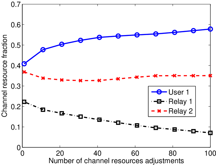
Fig. 6: The evolution of channel resource adjustment of the distributed control nodes with DF relaying.

In Algorithm 1, the channel allocation θ→\vec{\theta} is computed according to (27) after every K=2K=2 iterations, and the channel resources of the control nodes β→\vec{\beta} is adjusted according to (45) after every 1010 iterations. The algorithm parameters are chosen as cm=cm​j=10−4c_{m}=c_{mj}=10^{-4}, αl=5×10⁻⁵\alpha_{l}=5\times 10^{-5}, δ⁡(q)=0.3\delta(q)=0.3, and θmin=0.01\theta_{\min}=0.01. Our numerical experience suggests that there is a wide range of the algorithm parameters cmc_{m} and cm​jc_{mj} that ensures the convergence and optimality of Algorithm 1.

The spectrum efficiency and relay selection of each data stream are provided in Tab. I. Figure 4 illustrates the evolution of our resource allocation Algorithm 1. The total spectrum efficiency of the network increases 35.5% by deploying DF relay techniques. The convergence speeds of Algorithm 1 and traditional proximal point algorithm [31] are shown in Fig. 5. In the proximal point algorithm, the auxiliary update of (10) is implemented only after the updates of (8) and (9) converge and satisfy the criteria ‖ν→​(k+1)−ν→​(k)‖2≤0.01​‖ν→​(k)‖2\|\vec{\nu}(k+1)-\vec{\nu}(k)\|_{2}\leq 0.01\|\vec{\nu}(k)\|_{2}. Since Algorithm 1 has less layers of iterations than the proximal point algorithm, it has a much faster convergence speed. We note that this is the convergence speed when the algorithm is cold started. In practice, since the channel condition varies slowly, the resource allocation solution from the previous run of the algorithm is an excellent initial state. By using the previous solution for warm-starting the algorithm, the algorithm converges much faster.

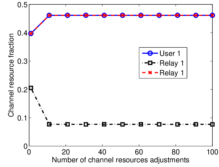
The evolution of the channel resource adjustment of the distributed control nodes, i.e., User 1, Relay 1, and Relay 2, is illustrated in Fig. 6 for the case that DF relay technique is employed, and in Fig. 7 for the case that the relay nodes only act as control nodes but not perform DF relaying.
Refer to caption
Fig. 7: The evolution of channel resource adjustment of the distributed control nodes without DF relaying.

VII Conclusion

In this paper, we have developed a distributed resource allocation algorithm to jointly optimize the power allocation, channel allocation and relay selection for DF relay networks with a large number of sources, relays, and destinations. Conventional dual decomposition techniques are not applicable, because the objective function is not strictly concave. We resolve this problem by adding some quadratic terms to make the objective function strictly concave. In this algorithm, information exchange only occurs locally among the source, relay, destination, and control nodes of each DF relay link. We have establish the convergence and optimality of our distributed resource allocation algorithm. A centralized channel resource adjustment algorithm has been developed on top of the distributive resource allocation algorithm to achieve traffic load balance. Numerical results are provided to illustrate the benefits of our proposed algorithm.

References

  • [1] A. Sendonaris, E. Erkip, and B. Aazhang, “User cooperation diversity- Part I: System description; Part II: Implementation aspects and performance analysis,” IEEE Trans. Commun., vol. 51, pp. 1927–1948, Nov. 2003.
  • [2] J. Laneman, D. Tse, and G. Wornell, “Cooperative diversity in wireless networks: Efficient protocols and outage behavior,” IEEE Trans. Inf. Theory, vol. 50, no. 12, pp. 3062–3080, Dec. 2004.
  • [3] S. Peters and R. Heath, “The future of WiMAX: Multihop relaying with IEEE 802.16j,” IEEE Commun. Mag., vol. 47, no. 1, pp. 104–111, 2009.
  • [4] K. Loa, C.-C. Wu, S.-T. Sheu, Y. Yuan, M. Chion, D. Huo, , and L. Xu, “IMT-Advanced relay standards,” IEEE Commun. Mag., vol. 48, no. 8, pp. 40–48, Aug. 2010.
  • [5] M. Salem, A. Adinoyi, M. Rahman, H. Yanikomeroglu, D. Falconer, Y.-D. Kim, E. Kim, and Y.-C. Cheong, “An overview of radio resource management in relay-enhanced OFDMA-based networks,” IEEE Commun. Surveys Tuts., vol. 12, no. 3, pp. 422–438, 2010.
  • [6] A. Hø{\o}st-Madsen and J. Zhang, “Capacity bounds and power allocation for wireless relay channels,” IEEE Trans. Inf. Theory, vol. 51, no. 6, pp. 2020–2040, Jun. 2005.
  • [7] Y. Zhao, R. Adve, and T. Lim, “Improving amplify-and-forward relay networks: optimal power allocation versus selection,” IEEE Trans. Wireless Commun., vol. 6, no. 8, pp. 3114–3123, Aug. 2007.
  • [8] Y. Liang, V. V. Veeravalli, and H. V. Poor, “Resource allocation for wireless fading relay channel: Max-min solution,” IEEE Trans. Inf. Theory, vol. 53, no. 10, pp. 3432–3453, Oct. 2007.
  • [9] Y.-W. Hong, W.-J. Huang, F.-H. Chiu, and C.-C. Kuo, “Cooperative communications in resource-constrained wireless networks,” IEEE Signal Process. Mag., vol. 24, no. 3, pp. 47–57, May 2007.
  • [10] J. Tang and X. Zhang, “Cross-layer resource allocation over wireless relay networks for quality of service provisioning,” IEEE J. Sel. Areas Commun., vol. 25, no. 5, pp. 645–656, May 2007.
  • [11] Y. Li, B. Vucetic, Z. Zhou, and M. Dohler, “Distributed adaptive power allocation for wireless relay networks,” IEEE Trans. Wireless Commun., vol. 6, no. 3, pp. 948–958, Mar. 2007.
  • [12] Z. Ding, W. H. Chin, and K. Leung, “Distributed beamforming and power allocation for cooperative networks,” IEEE Trans. Wireless Commun., vol. 7, no. 5, pp. 1817–1822, May 2008.
  • [13] M. Chen, S. Serbetli, and A. Yener, “Distributed power allocation strategies for parallel relay networks,” IEEE Trans. Wireless Commun., vol. 7, no. 2, pp. 552–561, Feb. 2008.
  • [14] W. Dang, M. Tao, H. Mu, and J. Huang, “Subcarrier-pair based resource allocation for cooperative multi-relay OFDM systems,” IEEE Trans. Wireless Commun., vol. 9, no. 5, pp. 1640–1649, May 2010.
  • [15] I. Maric and R. Yates, “Bandwidth and power allocation for cooperative strategies in gaussian relay networks,” IEEE Trans. Inf. Theory, vol. 56, no. 4, pp. 1880–1889, Apr. 2010.
  • [16] Y. Sun, X. Zhong, T.-H. Chang, S. Zhou, J. Wang, and C.-Y. Chi, “Real-time optimal spectrum sharing between cooperative relay and ad-hoc networks,” IEEE Trans. Signal Process., vol. 60, no. 4, pp. 1971–1985, Apr. 2012.
  • [17] G. Li and H. Liu, “Resource allocation for OFDMA relay networks with fairness constraints,” IEEE J. Sel. Areas Commun., vol. 24, no. 11, pp. 2061–2069, Nov. 2006.
  • [18] T. C.-Y. Ng and W. Yu, “Joint optimization of relay strategies and resource allocations in cooperative cellular networks,” IEEE J. Sel. Areas Commun., vol. 25, no. 2, pp. 328–339, Feb. 2007.
  • [19] L. Weng and R. Murch, “Cooperation strategies and resource allocations in multiuser OFDMA systems,” IEEE Trans. Veh. Technol., vol. 58, no. 5, pp. 2331–2342, Jun. 2009.
  • [20] K. Jitvanichphaibool, R. Zhang, and Y.-C. Liang, “Optimal resource allocation for two-way relay-assisted OFDMA,” IEEE Trans. Veh. Technol., vol. 58, no. 7, pp. 3311–3321, Sep. 2009.
  • [21] Y. Cui, V. Lau, and R. Wang, “Distributive subband allocation, power and rate control for relay-assisted OFDMA cellular system with imperfect system state knowledge,” IEEE Trans. Wireless Commun., vol. 8, no. 10, pp. 5096–5102, Oct. 2009.
  • [22] H. Li, H. Luo, X. Wang, C. Lin, and C. Li, “Fairness-aware resource allocation in ofdma cooperative relaying network,” in IEEE International Conference on Communications (ICC 2009), Jun 2009, pp. 1–5.
  • [23] X. Gong, S. Vorobyov, and C. Tellambura, “Joint bandwidth and power allocation with admission control in wireless multi-user networks with and without relaying,” IEEE Trans. Signal Process., vol. 59, no. 4, pp. 1801–1813, Apr. 2011.
  • [24] L. Le and E. Hossain, “Cross-layer optimization frameworks for multihop wireless networks using cooperative diversity,” IEEE Trans. Wireless Commun., vol. 7, no. 7, pp. 2592–2602, Jul. 2008.
  • [25] S. Kadloor and R. Adve, “Relay selection and power allocation in cooperative cellular networks,” IEEE Trans. Wireless Commun., vol. 9, no. 5, pp. 1676–1685, May 2010.
  • [26] K. Hosseini and R. Adve, “Relay selection and max-min resource allocation for multi-source OFDM-based mesh networks,” in IEEE International Conference on Communications (ICC 2010), May 2010, pp. 1–6.
  • [27] S. Serbetli and A. Yener, “Relay assisted F/TDMA ad hoc networks: Node classification, power allocation and relaying strategies,” IEEE Trans. Commun., vol. 56, no. 6, pp. 937–947, Jun. 2008.
  • [28] X. Lin, N. Shroff, and R. Srikant, “A tutorial on cross-layer optimization in wireless networks,” IEEE J. Sel. Areas Commun., vol. 24, no. 8, pp. 1452–1463, Aug. 2006.
  • [29] L. Xiao, M. Johansson, and S. P. Boyd, “Simultaneous routing and resource allocation via dual decomposition,” IEEE Trans. Commun., vol. 52, no. 7, pp. 1136–1144, Jul. 2004.
  • [30] W. Yu and R. Lui, “Dual methods for nonconvex spectrum optimization of multicarrier systems,” IEEE Trans. Commun., vol. 54, no. 7, pp. 1310–1322, Jul. 2006.
  • [31] D. P. Bertsekas and J. N. Tsitsiklis, Parallel and Distributed Computation: Numerical Methods. Englewood Cliffs, NJ: Prentice-Hall, 1989.
  • [32] X. Lin and N. Shroff, “Utility maximization for communication networks with multipath routing,” IEEE Trans. Auto. Control, vol. 51, no. 5, pp. 766–781, May 2006.
  • [33] D. Gündüz, E. Erkip, A. Goldsmith, and H. Poor, “Cooperative relaying in sensor networks,” in Proceedings of the Fifth International Conference on Cognitive Radio Oriented Wireless Networks Communications (CROWNCOM 2010), Jun. 2010, pp. 1–5.
  • [34] J. Kim, X. Lin, N. Shroff, and P. Sinha, “Minimizing delay and maximizing lifetime for wireless sensor networks with anycast,” IEEE/ACM Trans. Netw., vol. 18, no. 2, pp. 515–528, Apr. 2010.
  • [35] D. Tse and P. Viswanath, Fundamentals of Wireless Communications. Cambridge, UK: Cambridge University Press, 2005.
  • [36] D. P. Bertsekas, Nonlinear Programming, 2nd ed. Belmont, MA: Athena Scientific, 1999.
  • [37] S. Boyd and L. Vandenberghe, Convex Optimization. Cambridge, UK: Cambridge University Press, 2004.
  • [38] S. Boyd, L. Xiao, and A. Mutapcic, “Lecture notes of EE392o: Subgradient methods,” Stanford University, 2003. [Online]. Available: http://www.stanford.edu/class/ee392o
  • [39] D. Palomar and M. Chiang, “A tutorial on decomposition methods for network utility maximization,” IEEE J. Sel. Areas Commun., vol. 24, no. 8, pp. 1439–1451, Aug. 2006.
  • [40] ——, “Alternative distributed algorithms for network utility maximization: Framework and applications,” IEEE Trans. Auto. Control, vol. 52, no. 12, pp. 2254–2269, Dec. 2007.
  • [41] M. Bazaraa, H. Sherali, and C. Shetty, Nonlinear Programming: Theory and Algorithms, 3rd ed. Hoboken, New Jersey: Wiley-interscience, 2006.
  • [42] N. Z. Shor, Minimization Methods for Non-Differentiable Functions. New York, NY: Springer-Verlag New York, Inc., 1985.

-A Proof of Lemma 1

The Karush-Kuhn-Tucker (KKT) conditions [37] of (16) imply

gs,dln⁡2​(+gs,d​PsθD​T)−c⁡(Ps−Qs)−μ​{=0,if​Ps>0≤0,if​Ps=0.\displaystyle\frac{g^{s,d}}{\ln 2(1\!+\!\frac{g^{s,d}P^{s}}{\theta^{DT}})}\!-\!{c}\left(P^{s}-Q^{s}\right)\!-\!\mu\!\left\{\!\!\!\begin{array}[]{l}=0,\textrm{if}~P^{s}\!>\!0\\ \leq 0,\textrm{if}~P^{s}\!=\!0\end{array}\right.\!\!\!.\!\!\!

When Ps>0P^{s}>0, (-A) achieves equality, PsP^{s} is thus the positive root of a quadratic equation equivalent with (-A); otherwise, Ps=0P^{s}=0. Summarizing these two cases, the value of PsP^{s} is given by (18).

-B Proof of Lemma 2

Let us define the rate functions

R1=\displaystyle R_{1}= θD​F2​log2​[1+2​(Ps​gs,d+Pr​gr,d)θD​F],\displaystyle\frac{\theta^{DF}}{2}\log_{2}\left[1+\frac{2\left(P^{s}g^{s,d}+P^{r}g^{r,d}\right)}{\theta^{DF}}\right], (49)
R2=\displaystyle R_{2}= θD​F2​log2⁡(1+2​Ps​gs,rθD​F).\displaystyle\frac{\theta^{DF}}{2}\log_{2}\left(1+\frac{2P^{s}g^{s,r}}{\theta^{DF}}\right). (50)

Therefore, the achievable rate of DF relaying can be expressed as RD​F=min⁡{R1,R2}.R^{DF}=\min\left\{R_{1},R_{2}\right\}. Problem (17) is equivalent to the following problem:

maxt,Ps,Pr≥0\displaystyle\!\!\!\!\max_{\begin{subarray}{c}t,P^{s},P^{r}\geq 0\end{subarray}} t−c2​(Ps−Qs)2−c2​(Pr−Qr)2−μ​Ps−ν​Pr\displaystyle t\!-\!\frac{c}{2}\left(P^{s}\!-\!Q^{s}\right)^{2}\!-\!\frac{c}{2}\left(P^{r}\!-\!Q^{r}\right)^{2}\!-\!\mu P^{s}\!-\!\nu P^{r} (51a)
s.t.    t≤R1,t≤R2,\displaystyle t\leq R_{1},~~t\leq R_{2}, (51b)

where R1R_{1} and R2R_{2} are defined in (49) and (50). The Lagrangian of problem (51) is

L⁡(t,Ps,Pr,τ,ζ,μ,ν)\displaystyle L(t,P^{s},P^{r};\tau,\zeta,\mu,\nu)
=\displaystyle= t+τ⁡(R1−t)+ζ⁡(R2−t)−c2​(Ps−Qs)2\displaystyle t+\tau(R_{1}-t)+\zeta(R_{2}-t)-\frac{c}{2}\left(P^{s}-Q^{s}\right)^{2}
−c2​(Pr−Qr)2−μ​Ps−ν​Pr.\displaystyle-\frac{c}{2}\left(P^{r}-Q^{r}\right)^{2}-\mu P^{s}-\nu P^{r}. (52)

The KKT optimality conditions of problem (51) indicate

∂L∂t=1−τ−ζ=0,\displaystyle\frac{\partial L}{\partial t}=1-\tau-\zeta=0, (53)
τ≥0,R1−t≥0,τ⁡(R1−t)=0,\displaystyle\tau\geq 0,~R_{1}-t\geq 0,~\tau(R_{1}-t)=0, (54)
ζ≥0,R2−t≥0,ζ⁡(R2−t)=0.\displaystyle\zeta\geq 0,~R_{2}-t\geq 0,~\zeta(R_{2}-t)=0. (55)

By (53), the Lagrangian (52) can be simplified as

L⁡(Ps,Pr,τ,μ,ν)\displaystyle L(P^{s},P^{r};\tau,\mu,\nu)
=\displaystyle= τ​R1+(1−τ)​R2−c2​(Ps−Qs)2−c2​(Pr−Qr)2\displaystyle\tau R_{1}+(1-\tau)R_{2}-\frac{c}{2}\left(P^{s}-Q^{s}\right)^{2}-\frac{c}{2}\left(P^{r}-Q^{r}\right)^{2}
−μ​Ps−ν​Pr.\displaystyle-\mu P^{s}-\nu P^{r}. (56)

Moreover, from the KKT optimality conditions (53)-(55), we obtain

{ifR1⋆>R2⋆,τ=0;ifR1⋆<R2⋆,τ=1;ifR1⋆=R2⋆,0≤τ≤1,\displaystyle\left\{\begin{array}[]{l}\textrm{if}~~~R_{1}^{\star}>R_{2}^{\star},~~~\tau=0;\\ \textrm{if}~~~R_{1}^{\star}<R_{2}^{\star},~~~\tau=1;\\ \textrm{if}~~~R_{1}^{\star}=R_{2}^{\star},~~0\leq\tau\leq 1,\end{array}\right.

where R1⋆R_{1}^{\star} and R2⋆R_{2}^{\star} are corresponding rate values (49) and (50) at the optimal power allocation solution. Therefore, problem (51) can be address by solving the Lagrangian maximization problem

maxPs,Pr≥0⁡L⁡(Ps,Pr,τ,μ,ν),\displaystyle\max_{P^{s},P^{r}\geq 0}L(P^{s},P^{r};\tau,\mu,\nu), (60)

for the 3 cases expressed in (-B).

Case 1: When R1⋆>R2⋆,R_{1}^{\star}>R_{2}^{\star}, we have τ=0\tau=0. The KKT conditions of (60) are

gs,rln⁡2​(+2​gs,r​PsθD​F)−μ+c⁡(Ps−Qs)​{=0,if​Ps>0≤0,if​Ps=0,\displaystyle\frac{g^{s,r}}{\ln 2(1\!+\!\frac{2g^{s,r}{P}^{s}}{{\theta}^{DF}})}\!-\!\mu\!+\!c({P}^{s}\!-\!Q^{s})\!\left\{\!\!\!\begin{array}[]{l}=0,\textrm{if}~P^{s}\!>\!0\\ \leq 0,\textrm{if}~P^{s}\!=\!0\end{array}\right.\!\!\!,\!\!\!
−ν−c⁡(Pr−Qr)​{=0,if​Pr>0≤0,if​Pr=0.\displaystyle-\nu-c({P}^{r}-Q^{r})\left\{\begin{array}[]{l}=0,\textrm{if}~P^{r}>0\\ \leq 0,\textrm{if}~P^{r}=0\end{array}\right..

The solution to (-B) is similar to that of  (-A). Further considering (-B), the optimal source and relay power is given by (22). Note that Case 1 requires R1⋆>R2⋆R_{1}^{\star}>R_{2}^{\star}, which can be equivalently expressed by gr,d​Pr>(gs,r−gs,d)​Psg^{r,d}P^{r}>(g^{s,r}-g^{s,d})P^{s}.

Case 2: When R1⋆<R2⋆,R_{1}^{\star}<R_{2}^{\star}, τ=1\tau=1. The KKT conditions of  (60) are given by

gs,dln⁡2​(1+2​gs,d​Ps+2​gr,d​PrθD​F)−μ−c⁡(Ps−Qs)\displaystyle\frac{g^{s,d}}{\ln 2(1+\frac{2g^{s,d}{P}^{s}+2g^{r,d}{P}^{r}}{\theta^{DF}})}-\mu-c({P}^{s}-Q^{s})
{=0,if​Ps>0≤0,if​Ps=0,\displaystyle~~~~~~~~~~~~~~~~~~~~~~~~~~~~~~~~~~~~\left\{\begin{array}[]{l}=0,~\textrm{if}~P^{s}>0\\ \leq 0,~\textrm{if}~P^{s}=0\end{array}\right.,
gr,dln⁡2​(1+2​gs,d​Ps+2​gr,d​PrθD​F)−ν−c⁡(Pr−Qr)\displaystyle\frac{g^{r,d}}{\ln 2(1+\frac{2g^{s,d}{P}^{s}+2g^{r,d}{P}^{r}}{\theta^{DF}})}-\nu-c({P}^{r}-Q^{r})
{=0,if​Pr>0≤0,if​Pr=0.\displaystyle~~~~~~~~~~~~~~~~~~~~~~~~~~~~~~~~~~~~\left\{\begin{array}[]{l}=0,~\textrm{if}~P^{r}>0\\ \leq 0,~\textrm{if}~P^{r}=0\end{array}\right..

If Ps>0,Pr>0P^{s}>0,P^{r}>0, then (-B) and (-B) take equality. By viewing e=gs,d​Ps+gr,d​Pre=g^{s,d}{P}^{s}+g^{r,d}{P}^{r} as a whole body, we can get a quadratic equation of ee from (-B) and (-B), which has a positive root given by (24). Moreover, by comparing (-B) and (-B) with equality, we obtain

[μ+c⁡(Ps−Qs)]​gr,d=[ν+c⁡(Pr−Qr)]​gs,d.\displaystyle\left[\mu+c({P}^{s}-Q^{s})\right]g^{r,d}=\left[\nu+c({P}^{r}-Q^{r})\right]g^{s,d}. (69)

Substituting (69) into (24), the optimal power allocation solution is derived as in (23).

If Pr=0P^{r}=0, (-B) reduces to a formula similar with (-B), and its solution is given by (25).

Note that Case 2 requires R1⋆<R2⋆R_{1}^{\star}<R_{2}^{\star}, which is guaranteed by gr,d​Pr<(gs,r−gs,d)​Psg^{r,d}P^{r}<(g^{s,r}-g^{s,d})P^{s}. The case of Ps=0P^{s}=0 and Pr>0P^{r}>0 cannot happen, since it violates the condition R1⋆<R2⋆R_{1}^{\star}<R_{2}^{\star}.

Case 3: If R1⋆=R2⋆R_{1}^{\star}=R_{2}^{\star}, the KKT conditions of (60) are given by

τ​gs,dln⁡2​(+2​gs,d​Ps+2​gr,d​PrθD​F)+(1−τ)​gs,rln⁡2​(+2​gs,r​PsθD​F)\displaystyle\frac{\tau g^{s,d}}{\ln 2(1\!+\!\frac{2g^{s,d}{P}^{s}+\!2g^{r,d}{P}^{r}}{\theta^{DF}})}\!+\!\frac{(1-\tau)g^{s,r}}{\ln 2(1\!+\frac{2g^{s,r}{P}^{s}}{{\theta}^{DF}})}
−μ−c⁡(Ps−Qs)​{=0,if​Ps>0≤0,if​Ps=0,\displaystyle~~~~~~~~~~~~~~~~-\mu-c({P}^{s}-Q^{s})\left\{\begin{array}[]{l}=0,~\textrm{if}~P^{s}>0\\ \leq 0,~\textrm{if}~P^{s}=0\end{array}\right.,
τ​gr,dln⁡2​(1+2​gs,d​Ps+2​gr,d​PrθD​F)\displaystyle\frac{\tau g^{r,d}}{\ln 2(1+\frac{2g^{s,d}{P}^{s}+2g^{r,d}{P}^{r}}{\theta^{DF}})}
−ν−c⁡(Pr−Qr)​{=0,if​Pr>0≤0,if​Pr=0.\displaystyle~~~~~~~~~~~~~~~~-\nu-c({P}^{r}-Q^{r})\left\{\begin{array}[]{l}=0,~\textrm{if}~P^{r}>0\\ \leq 0,~\textrm{if}~P^{r}=0\end{array}\right..

Since R1⋆=R2⋆R_{1}^{\star}=R_{2}^{\star}, we have

gr,d​Pr=(gs,r−gs,d)​Ps.\displaystyle g^{r,d}P^{r}=(g^{s,r}-g^{s,d})P^{s}. (74)

If Ps>0,Pr>0P^{s}>0,P^{r}>0, both (-B) and (-B) achieves equality. By substituting (74) into (-B) and (-B), we can eliminate τ\tau and derive the optimal values of PsP^{s} and PrP^{r}. Otherwise, Ps=Pr=0P^{s}=P^{r}=0. These two cases are summarized in (26).

-C Proof of Lemma 3

We proceed to show the inequalities

[∇PmsRmD​T(Pm,1s)−∇PmsRmD​T(Qms∗)]T(Pm,2s−Qms∗)\displaystyle\Big[\nabla_{{P}^{s}_{m}}R_{m}^{DT}({P}^{s}_{m,1})-\nabla_{{P}^{s}_{m}}R_{m}^{DT}({Q}_{m}^{s*})\Big]^{T}\big({P}^{s}_{m,2}-{Q}_{m}^{s*}\big)
≤12​cm​(μs⁡(m),2−μs⁡(m),1)2,∀m,\displaystyle\leq\frac{1}{2c_{m}}(\mu_{s(m),2}-\mu_{s(m),1})^{2},\forall m, (75)

and

[∇P→m​jRm​jD​F​(P→m​j,1)−∇P→m​jRm​jD​F​(Q→m​j∗)]T​(P→m​j,2−Q→m​j∗)\displaystyle\Big[\nabla_{\vec{P}_{mj}}R_{mj}^{DF}(\vec{P}_{mj,1})-\nabla_{\vec{P}_{mj}}R_{mj}^{DF}(\vec{Q}_{mj}^{*})\Big]^{T}\big(\vec{P}_{mj,2}-\vec{Q}_{mj}^{*}\big)\!\!\!
≤12​cm​j​[(μs⁡(m),2−μs⁡(m),1)2+(νj,2−νj,1)2],∀m,j,\displaystyle\leq\frac{1}{2c_{mj}}\left[(\mu_{s(m),2}-\mu_{s(m),1})^{2}+(\nu_{j,2}-\nu_{j,1})^{2}\right],\forall m,j, (76)

where Pm,is{P}^{s}_{m,i} is the maximizer of (16) corresponding to the multiplier μs⁡(m),i\mu_{s(m),i} for i∈{1,2}i\in\{1,2\}, and P→m​j,i=(Pm​j,is,Pm​j,ir)\vec{P}_{mj,i}=(P_{mj,i}^{s},P_{mj,i}^{r}) is the maximizer of (17) corresponding the multiplier (μs⁡(m),i,νj,i)(\mu_{s(m),i},\nu_{j,i}). The asserted result (38) follows, if we take the summation of the inequalities (75) and (76) for all the possible choices of mm and jj. Since RmD​TR_{m}^{DT} is a concave function of a single variable PmsP_{m}^{s}, the techniques of [32] can be directly used here to prove (75). In the sequel, we will show (76) for each DF relay link. Since we only need to focus on one DF relay link, the subscripts m,j,s⁡(m)m,j,s(m) are omitted in the sequel to facilitate our expressions.

Let us associate Lagrange multipliers Ls≥0L^{s}\geq 0 and Lr≥0L^{r}\geq 0 for the constraints Ps≥0P^{s}\geq 0 and Pr≥0P^{r}\geq 0, respectively, in the maximization of (17). Using the Karush-Kuhn-Tucker condition, we can conclude that there must exist a subgradient (∂RD​F​(P→)∂Ps,∂RD​F​(P→)∂Pr)(\frac{\partial R^{DF}(\vec{P})}{\partial P^{s}},\frac{\partial R^{DF}(\vec{P})}{\partial P^{r}}) of RD​FR^{DF} such that

∂RD​F​(P→)∂Ps−μ−c⁡(Ps−Qs)+Ls=0,\displaystyle\frac{\partial R^{DF}(\vec{P})}{\partial P^{s}}-\mu-c(P^{s}-Q^{s})+L^{s}=0, (77)
∂RD​F​(P→)∂Pr−ν−c⁡(Pr−Qr)+Lr=0,\displaystyle\frac{\partial R^{DF}(\vec{P})}{\partial P^{r}}-\nu-c(P^{r}-Q^{r})+L^{r}=0, (78)
Ls​Ps=0,Lr​Pr=0,\displaystyle L^{s}P^{s}=0,~~~L^{r}P^{r}=0, (79)

where P→=(Ps,Pr)\vec{P}=(P^{s},P^{r}) represents the source and relay power of the considered DF relay link. From (39) and (40), we also have

∇PsRD​F​(P→)−μ−c⁡(Ps−Qs)=0,\displaystyle\nabla_{{P}^{s}}R^{DF}(\vec{P})-\mu-c(P^{s}-Q^{s})=0, (80)
∇PrRD​F​(P→)−ν−c⁡(Pr−Qr)=0.\displaystyle\nabla_{{P}^{r}}R^{DF}(\vec{P})-\nu-c(P^{r}-Q^{r})=0. (81)

Comparing (77) and (78) with (80) and (81), we see that

∇PsRD​F​(P→)=∂RD​F​(P→)∂Ps+Ls,\displaystyle\nabla_{{P}^{s}}R^{DF}(\vec{P})=\frac{\partial R^{DF}(\vec{P})}{\partial P^{s}}+L^{s},
∇PrRD​F​(P→)=∂RD​F​(P→)∂Pr+Lr.\displaystyle\nabla_{{P}^{r}}R^{DF}(\vec{P})=\frac{\partial R^{DF}(\vec{P})}{\partial P^{r}}+L^{r}.

Let Q→∗=(Qs∗,Qr∗)\vec{Q}^{*}=(Q^{s*},Q^{r*}) be the source and relay power at the stationary point. Similarly, we can obtain

∇PsRD​F(Q→∗)=∂RD​F​(Q→∗)∂Ps+Ls∗,\displaystyle\nabla_{{P}^{s}}R^{DF}(\vec{Q}^{*})=\frac{\partial R^{DF}(\vec{Q}^{*})}{\partial P^{s}}+L^{s*},
∇PrRD​F(Q→∗)=∂RD​F​(Q→∗)∂Pr+Lr∗.\displaystyle\nabla_{{P}^{r}}R^{DF}(\vec{Q}^{*})=\frac{\partial R^{DF}(\vec{Q}^{*})}{\partial P^{r}}+L^{r*}.

Then, we further have

[∇RD​F​(P→1)−∇RD​F​(Q→∗)]T​(P→2−Q→∗)\displaystyle\Big[\nabla R^{DF}(\vec{P}_{1})-\nabla R^{DF}(\vec{Q}^{*})\Big]^{T}\big(\vec{P}_{2}-\vec{Q}^{*}\big)
=\displaystyle\!\!\!= [∂RD​F​(P→1)∂Ps−∂RD​F​(Q→∗)∂Ps](P2s−Qs∗)\displaystyle\Big[\frac{\partial R^{DF}(\vec{P}_{1})}{\partial P^{s}}-\frac{\partial R^{DF}(\vec{Q}^{*})}{\partial P^{s}}\Big](P_{2}^{s}-Q^{s*})
+[∂RD​F​(P→1)∂Pr−∂RD​F​(Q→∗)∂Pr](P2r−Qr∗)\displaystyle+\Big[\frac{\partial R^{DF}(\vec{P}_{1})}{\partial P^{r}}-\frac{\partial R^{DF}(\vec{Q}^{*})}{\partial P^{r}}\Big](P_{2}^{r}-Q^{r*})
+(L1s−Ls∗)(P2s−Qs∗)+(L1r−Lr∗)(P2r−Qr∗).\displaystyle+\big(L_{1}^{s}\!-\!L^{s*}\big)\big(P_{2}^{s}\!-\!Q^{s*}\big)+\big(L_{1}^{r}\!-\!L^{r*}\big)\big(P_{2}^{r}\!-\!Q^{r*}\big).

We can use the arguments in [32] to show that

(L1s−Ls∗)(P2s−Qs∗)+(L1r−Lr∗)(P2r−Qr∗)\displaystyle\big(L_{1}^{s}\!-\!L^{s*}\big)\big(P_{2}^{s}\!-\!Q^{s*}\big)+\big(L_{1}^{r}\!-\!L^{r*}\big)\big(P_{2}^{r}\!-\!Q^{r*}\big)
≤\displaystyle\leq 14​c​[(μ2−μ1)2+(ν2−ν1)2].\displaystyle\frac{1}{4c}\left[(\mu_{2}-\mu_{1})^{2}+(\nu_{2}-\nu_{1})^{2}\right].

Now we only need to show

[∂RD​F​(P→1)∂Ps−∂RD​F​(Q→∗)∂Ps](P2s−Qs∗)\displaystyle\Big[\frac{\partial R^{DF}(\vec{P}_{1})}{\partial P^{s}}-\frac{\partial R^{DF}(\vec{Q}^{*})}{\partial P^{s}}\Big](P_{2}^{s}-Q^{s*})
+\displaystyle\!\!\!\!+ [∂RD​F​(P→1)∂Pr−∂RD​F​(Q→∗)∂Pr](P2r−Qr∗)\displaystyle\Big[\frac{\partial R^{DF}(\vec{P}_{1})}{\partial P^{r}}-\frac{\partial R^{DF}(\vec{Q}^{*})}{\partial P^{r}}\Big](P_{2}^{r}-Q^{r*})
≤\displaystyle\leq 14​c​[(μ2−μ1)2+(ν2−ν1)2].\displaystyle\frac{1}{4c}\left[(\mu_{2}-\mu_{1})^{2}+(\nu_{2}-\nu_{1})^{2}\right]. (82)

for (76) to hold.

Let us further define

a1s=\displaystyle a_{1}^{s}= ∂RD​F​(P→1)∂Ps−∂RD​F​(Q→∗)∂Ps,b1s=P1s−Qs∗,\displaystyle\frac{\partial R^{DF}(\vec{P}_{1})}{\partial P^{s}}-\frac{\partial R^{DF}(\vec{Q}^{*})}{\partial P^{s}},~~b_{1}^{s}=P_{1}^{s}-Q^{s*},
a1r=\displaystyle a_{1}^{r}= ∂RD​F​(P→1)∂Pr−∂RD​F​(Q→∗)∂Pr,b1r=P1r−Qr∗,\displaystyle\frac{\partial R^{DF}(\vec{P}_{1})}{\partial P^{r}}-\frac{\partial R^{DF}(\vec{Q}^{*})}{\partial P^{r}},~~b_{1}^{r}=P_{1}^{r}-Q^{r*},
a2s=\displaystyle a_{2}^{s}= ∂RD​F​(P→2)∂Ps−∂RD​F​(Q→∗)∂Ps,b2s=P2s−Qs∗\displaystyle\frac{\partial R^{DF}(\vec{P}_{2})}{\partial P^{s}}-\frac{\partial R^{DF}(\vec{Q}^{*})}{\partial P^{s}},~~b_{2}^{s}=P_{2}^{s}-Q^{s*}
a2r=\displaystyle a_{2}^{r}= ∂RD​F​(P→2)∂Pr−∂RD​F​(Q→∗)∂Pr,b2r=P2r−Qr∗.\displaystyle\frac{\partial R^{DF}(\vec{P}_{2})}{\partial P^{r}}-\frac{\partial R^{DF}(\vec{Q}^{*})}{\partial P^{r}},~~b_{2}^{r}=P_{2}^{r}-Q^{r*}.

For ease of notation, let us define γs≜−L2s−L1sc⁡(P2s−P1s)≥0\gamma_{s}\triangleq-\frac{L_{2}^{s}-L_{1}^{s}}{c(P_{2}^{s}-P_{1}^{s})}\geq 0, γr≜−L2r−L1rc⁡(P2r−P1r)≥0\gamma_{r}\triangleq-\frac{L_{2}^{r}-L_{1}^{r}}{c(P_{2}^{r}-P_{1}^{r})}\geq 0, γs0≜1+γs\gamma_{s}^{0}\triangleq 1+\gamma_{s}, and γr0≜1+γr\gamma_{r}^{0}\triangleq 1+\gamma_{r}. Then, according to (77) and (78), we have

μ2−μ1\displaystyle\mu_{2}-\mu_{1} =a2s−a1s+c⁡(b1s−b2s)+L2s−L1s\displaystyle=a_{2}^{s}-a_{1}^{s}+c(b_{1}^{s}-b_{2}^{s})+L_{2}^{s}-L_{1}^{s} (83)
=(a1s−a2s)−c​γs0​(b1s−b2s),\displaystyle=\big(a_{1}^{s}-a_{2}^{s}\big)-c\gamma_{s}^{0}\big(b_{1}^{s}-b_{2}^{s}\big), (84)
ν2−ν1\displaystyle\nu_{2}-\nu_{1} =a2r−a1r+c⁡(b1r−b2r)+L2r−L1r\displaystyle=a_{2}^{r}-a_{1}^{r}+c(b_{1}^{r}-b_{2}^{r})+L_{2}^{r}-L_{1}^{r} (85)
=(a1r−a2r)−c​γs0​(b1r−b2r).\displaystyle=\big(a_{1}^{r}-a_{2}^{r}\big)-c\gamma_{s}^{0}\big(b_{1}^{r}-b_{2}^{r}\big). (86)

Moreover, (82) can be equivalently expressed as

a1s​b2s+a1r​b2r≤14​c​[(μ2−μ1)2+(ν2−ν1)2].a_{1}^{s}b_{2}^{s}+a_{1}^{r}b_{2}^{r}\leq\frac{1}{4c}\Big[(\mu_{2}-\mu_{1})^{2}+(\nu_{2}-\nu_{1})^{2}\Big]. (87)

The concavity of RD​FR^{DF} in (Ps,Pr)(P^{s},P^{r}) suggests

a1s​b1s+a1r​b1r≤0,a2s​b2s+a2r​b2r≤0.\displaystyle a_{1}^{s}b_{1}^{s}+a_{1}^{r}b_{1}^{r}\leq 0,~a_{2}^{s}b_{2}^{s}+a_{2}^{r}b_{2}^{r}\leq 0. (88)

If ais​bis≤0a_{i}^{s}b_{i}^{s}\leq 0 and air​bir≤0a_{i}^{r}b_{i}^{r}\leq 0 (i=1,2i=1,2), one can show Lemma 3 according to the arguments in [32]. However, rather than having ais​bis≤0a_{i}^{s}b_{i}^{s}\leq 0 or air​bir≤0a_{i}^{r}b_{i}^{r}\leq 0, we only have (88). In order to handle the difficulty, we will discuss case by case to fully explore the structure of RD​FR^{DF} defined in (2). In particular, we proceed the remaining proof by breaking into three levels of cases:

  • 1)

    Break into Case 1-7 based on all combinations of the signs of a1s​b1sa_{1}^{s}b_{1}^{s}, a1r​b1ra_{1}^{r}b_{1}^{r}, a2s​b2sa_{2}^{s}b_{2}^{s}, and a2r​b2ra_{2}^{r}b_{2}^{r}.

  • 2)

    In some cases, further break into subcases (I)-(IV) based on all combinations of the signs of a1s​b2sa_{1}^{s}b_{2}^{s} and a1r​b2ra_{1}^{r}b_{2}^{r}.

  • 3)

    In some subcases, further break into mini-cases (1)-(8) based on all combinations of P→1\vec{P}_{1}, P→2\vec{P}_{2}, and Q→∗\vec{Q}^{*} lying in region ①\textcircled{1} or region ②\textcircled{2}, where region ①\textcircled{1} is defined as RD​F=R1R^{DF}=R_{1}, i.e., gs,d​Ps+gr,d​Pr≤gs,r​Psg^{s,d}P^{s}+g^{r,d}P^{r}\leq g^{s,r}P^{s}, and region ②\textcircled{2} is defined as RD​F=R2R^{DF}=R_{2}, i.e., gs,d​Ps+gr,d​Pr≥gs,r​Psg^{s,d}P^{s}+g^{r,d}P^{r}\geq g^{s,r}P^{s}.

We will explain in detail how to prove (87) for each subcase and mini-case in Case 1, and also in relative detail for Case 2 to show that the proofs in Case 1 and Case 2 have similar logic. Since the techniques in Case 3-7 are quite similar with that used in Case 1, we will omit most of the similar steps without repeating the same proof logic.

Case 1: When a1s​b1s≥0,a1r​b1r≤0,a2s​b2s≤0,a2r​b2r≥0a_{1}^{s}b_{1}^{s}\geq 0,~a_{1}^{r}b_{1}^{r}\leq 0,~a_{2}^{s}b_{2}^{s}\leq 0,~a_{2}^{r}b_{2}^{r}\geq 0.
(I) We first assume a1s​b2s≥0,a1r​b2r≥0a_{1}^{s}b_{2}^{s}\geq 0,~a_{1}^{r}b_{2}^{r}\geq 0, then we have a1s​a2s≤0,b1s​b2s≥0,a1r​a2r≥0,b1r​b2r≤0a_{1}^{s}a_{2}^{s}\leq 0,~b_{1}^{s}b_{2}^{s}\geq 0,~a_{1}^{r}a_{2}^{r}\geq 0,~b_{1}^{r}b_{2}^{r}\leq 0. Now we further break into mini-cases:
(1) P→1\vec{P}_{1} is in region ①\textcircled{1}, P→2\vec{P}_{2} is in region ①\textcircled{1}, Q→∗\vec{Q}^{*} is in region ①\textcircled{1}. Then,

a1s=\displaystyle a_{1}^{s}= gs,d1+2θ​(gs,d​P1s+gr,d​P1r)−gs,d1+2θ(gs,dQs∗+gr,dQr∗),\displaystyle\frac{g^{s,d}}{1+\frac{2}{\theta}(g^{s,d}P_{1}^{s}+g^{r,d}P_{1}^{r})}-\frac{g^{s,d}}{1+\frac{2}{\theta}(g^{s,d}Q^{s*}+g^{r,d}Q^{r*})},
a1r=\displaystyle a_{1}^{r}= gr,d1+2θ​(gs,d​P1s+gr,d​P1r)−gr,d1+2θ(gs,dQs∗+gr,dQr∗),\displaystyle\frac{g^{r,d}}{1+\frac{2}{\theta}(g^{s,d}P_{1}^{s}+g^{r,d}P_{1}^{r})}-\frac{g^{r,d}}{1+\frac{2}{\theta}(g^{s,d}Q^{s*}+g^{r,d}Q^{r*})},
b1s=\displaystyle b_{1}^{s}= P1s−Qs∗,b1r=P1r−Qr∗,\displaystyle P_{1}^{s}-Q^{s*},~~~b_{1}^{r}=P_{1}^{r}-Q^{r*},
a2s=\displaystyle a_{2}^{s}= gs,d1+2θ​(gs,d​P2s+gr,d​P2r)−gs,d1+2θ(gs,dQs∗+gr,dQr∗),\displaystyle\frac{g^{s,d}}{1+\frac{2}{\theta}(g^{s,d}P_{2}^{s}+g^{r,d}P_{2}^{r})}-\frac{g^{s,d}}{1+\frac{2}{\theta}(g^{s,d}Q^{s*}+g^{r,d}Q^{r*})},
a2r=\displaystyle a_{2}^{r}= gr,d1+2θ​(gs,d​P2s+gr,d​P2r)−gr,d1+2θ(gs,dQs∗+gr,dQr∗),\displaystyle\frac{g^{r,d}}{1+\frac{2}{\theta}(g^{s,d}P_{2}^{s}+g^{r,d}P_{2}^{r})}-\frac{g^{r,d}}{1+\frac{2}{\theta}(g^{s,d}Q^{s*}+g^{r,d}Q^{r*})},
b2s=\displaystyle b_{2}^{s}= P2s−Qs∗,b2r=P2r−Qr∗.\displaystyle P_{2}^{s}-Q^{s*},~~~b_{2}^{r}=P_{2}^{r}-Q^{r*}.

If b1s≥0b_{1}^{s}\geq 0 and b1r≤0b_{1}^{r}\leq 0, then we must have b2s≥0b_{2}^{s}\geq 0 and b2r≥0b_{2}^{r}\geq 0 from b1s​b2s≥0b_{1}^{s}b_{2}^{s}\geq 0 and b1r​b2r≤0b_{1}^{r}b_{2}^{r}\leq 0, respectively. From the format of a2ra_{2}^{r}, we further get a2r≤0a_{2}^{r}\leq 0, which contradicts a2r​b2r≥0a_{2}^{r}b_{2}^{r}\geq 0;
If b1s≤0b_{1}^{s}\leq 0 and b1r≥0b_{1}^{r}\geq 0, then b2s≤0b_{2}^{s}\leq 0 and b2r≤0b_{2}^{r}\leq 0. Further, from the format of a2ra_{2}^{r}, we have a2r≥0a_{2}^{r}\geq 0, which contradicts a2r​b2r≥0a_{2}^{r}b_{2}^{r}\geq 0;
If b1s≥0b_{1}^{s}\geq 0 and b1r≥0b_{1}^{r}\geq 0, then from the format of a1sa_{1}^{s}, we have a1s≤0a_{1}^{s}\leq 0, which contradicts a1s​b1s≥0a_{1}^{s}b_{1}^{s}\geq 0;
If b1s≤0b_{1}^{s}\leq 0 and b1r≤0b_{1}^{r}\leq 0, then a1s≥0a_{1}^{s}\geq 0, which contradicts a1s​b1s≥0a_{1}^{s}b_{1}^{s}\geq 0.
Thus, mini-case (1) is impossible under Case 1.
(2) P→1\vec{P}_{1} is in region ①\textcircled{1}, P→2\vec{P}_{2} is in region ②\textcircled{2}, Q→∗\vec{Q}^{*} is in region ①\textcircled{1}. Then,

a1s=\displaystyle a_{1}^{s}= gs,d1+2θ​(gs,d​P1s+gr,d​P1r)−gs,d1+2θ(gs,dQs∗+gr,dQr∗),\displaystyle\frac{g^{s,d}}{1+\frac{2}{\theta}(g^{s,d}P_{1}^{s}+g^{r,d}P_{1}^{r})}-\frac{g^{s,d}}{1+\frac{2}{\theta}(g^{s,d}Q^{s*}+g^{r,d}Q^{r*})},
a1r=\displaystyle a_{1}^{r}= gr,d1+2θ​(gs,d​P1s+gr,d​P1r)−gr,d1+2θ(gs,dQs∗+gr,dQr∗),\displaystyle\frac{g^{r,d}}{1+\frac{2}{\theta}(g^{s,d}P_{1}^{s}+g^{r,d}P_{1}^{r})}-\frac{g^{r,d}}{1+\frac{2}{\theta}(g^{s,d}Q^{s*}+g^{r,d}Q^{r*})},
b1s=\displaystyle b_{1}^{s}= P1s−Qs∗,b1r=P1r−Qr∗,\displaystyle P_{1}^{s}-Q^{s*},~~~b_{1}^{r}=P_{1}^{r}-Q^{r*},
a2s=\displaystyle a_{2}^{s}= gs,r1+2θ​gs,r​P2s−gs,d1+2θ(gs,dQs∗+gr,dQr∗),\displaystyle\frac{g^{s,r}}{1+\frac{2}{\theta}g^{s,r}P_{2}^{s}}-\frac{g^{s,d}}{1+\frac{2}{\theta}(g^{s,d}Q^{s*}+g^{r,d}Q^{r*})},
a2r=\displaystyle a_{2}^{r}= −gr,d1+2θ(gs,dQs∗+gr,dQr∗),\displaystyle-\frac{g^{r,d}}{1+\frac{2}{\theta}(g^{s,d}Q^{s*}+g^{r,d}Q^{r*})},
b2s=\displaystyle b_{2}^{s}= P2s−Qs∗,b2r=P2r−Qr∗.\displaystyle P_{2}^{s}-Q^{s*},~~~b_{2}^{r}=P_{2}^{r}-Q^{r*}.

Refer to caption

Fig. 8: Illustration of Power Vector Regions for Case 1.(I).(1)

Since a2r≤0a_{2}^{r}\leq 0, we get b2r≤0b_{2}^{r}\leq 0 from a2r​b2r≥0a_{2}^{r}b_{2}^{r}\geq 0 and b1r≥0b_{1}^{r}\geq 0 from b1r​b2r≤0b_{1}^{r}b_{2}^{r}\leq 0. Suppose b1s≥0b_{1}^{s}\geq 0, then from the format of a1sa_{1}^{s}, we have a1s≤0a_{1}^{s}\leq 0 which contradicts a1s​b1s≥0a_{1}^{s}b_{1}^{s}\geq 0, so b1s≤0b_{1}^{s}\leq 0. By b1s​b2s≥0b_{1}^{s}b_{2}^{s}\geq 0, we also have b2s≤0b_{2}^{s}\leq 0. With the above facts and Figure. 8, we have P2s≤P1sP_{2}^{s}\leq P_{1}^{s}, i.e., b2s≤b1s≤0b_{2}^{s}\leq b_{1}^{s}\leq 0. It is apparent that a2r≤a1r≤0a_{2}^{r}\leq a_{1}^{r}\leq 0, and a1s≤0≤a2sa_{1}^{s}\leq 0\leq a_{2}^{s}.

Suppose P1s=0P_{1}^{s}=0, then P→1\vec{P}_{1} is on the boundary of region ①\textcircled{1} and ②\textcircled{2}, and it belongs to mini-case (4) later. Without loss of generality, let P1s≠0P_{1}^{s}\neq 0, and then L1s=0,(a2s−a1s)​(L2s−L1s)=(a2s−a1s)​L2s≥0L_{1}^{s}=0,~(a_{2}^{s}-a_{1}^{s})(L_{2}^{s}-L_{1}^{s})=(a_{2}^{s}-a_{1}^{s})L_{2}^{s}\geq 0. Similarly, P2r≠0,L2r=0P_{2}^{r}\neq 0,~L_{2}^{r}=0, and (a2r−a1r)​(L2r−L1r)=(a1r−a2r)​L1r≥0(a_{2}^{r}-a_{1}^{r})(L_{2}^{r}-L_{1}^{r})=(a_{1}^{r}-a_{2}^{r})L_{1}^{r}\geq 0. Also, a1s​b1s+a1r​b1r+a2s​b2s+a2r​b2r≤0a_{1}^{s}b_{1}^{s}+a_{1}^{r}b_{1}^{r}+a_{2}^{s}b_{2}^{s}+a_{2}^{r}b_{2}^{r}\leq 0. Thus, we have

14​c​[(μ2−μ1)2+(ν2−ν1)2]−a1s​b2s−a1r​b2r\displaystyle\frac{1}{4c}\Big[(\mu_{2}-\mu_{1})^{2}+(\nu_{2}-\nu_{1})^{2}\Big]-a_{1}^{s}b_{2}^{s}-a_{1}^{r}b_{2}^{r}
=\displaystyle= 14​c​(a2s−a1s)2+[c⁡(b1s−b2s)+L2s−L1s]24​c+\displaystyle\frac{1}{4c}(a_{2}^{s}-a_{1}^{s})^{2}+\frac{\big[c(b_{1}^{s}-b_{2}^{s})+L_{2}^{s}-L_{1}^{s}\big]^{2}}{4c}+
12​c​(a2s−a1s)​(L2s−L1s)−12​(a1s​b2s−a2s​b1s)+\displaystyle\frac{1}{2c}(a_{2}^{s}-a_{1}^{s})(L_{2}^{s}-L_{1}^{s})-\frac{1}{2}(a_{1}^{s}b_{2}^{s}-a_{2}^{s}b_{1}^{s})+
14​c​(a2r−a1r)2+[c⁡(b1r−b2r)+L2r−L1r]24​c+\displaystyle\frac{1}{4c}(a_{2}^{r}-a_{1}^{r})^{2}+\frac{\big[c(b_{1}^{r}-b_{2}^{r})+L_{2}^{r}-L_{1}^{r}\big]^{2}}{4c}+
12​c​(a2r−a1r)​(L2r−L1r)−12​(a1r​b2r−a2r​b1r)−\displaystyle\frac{1}{2c}(a_{2}^{r}-a_{1}^{r})(L_{2}^{r}-L_{1}^{r})-\frac{1}{2}(a_{1}^{r}b_{2}^{r}-a_{2}^{r}b_{1}^{r})-
12​(a1s​b1s+a1r​b1r+a2s​b2s+a2r​b2r)\displaystyle\frac{1}{2}(a_{1}^{s}b_{1}^{s}+a_{1}^{r}b_{1}^{r}+a_{2}^{s}b_{2}^{s}+a_{2}^{r}b_{2}^{r})
≥\displaystyle\geq 14​c​(a2r−a1r)2−12​(a1s​b2s−a2s​b1s+a1r​b2r−a2r​b1r).\displaystyle\frac{1}{4c}(a_{2}^{r}-a_{1}^{r})^{2}-\frac{1}{2}(a_{1}^{s}b_{2}^{s}-a_{2}^{s}b_{1}^{s}+a_{1}^{r}b_{2}^{r}-a_{2}^{r}b_{1}^{r}).

We want to choose cc carefully such that the above term is nonnegative. Since Q→∗\vec{Q}^{*} is feasible and Qs∗Q^{s*} should be bounded by PmaxsP_{{\max}}^{s}, we have a1s​b2s−a2s​b1s≤gs,dQs∗1+2θ(gs,dQs∗+gr,dQr∗)+gs,rQs∗1+2θ​gs,r​P2s≤12+gs,r​Pmaxsa_{1}^{s}b_{2}^{s}-a_{2}^{s}b_{1}^{s}\leq\frac{g^{s,d}Q^{s*}}{1+\frac{2}{\theta}(g^{s,d}Q^{s*}+g^{r,d}Q^{r*})}+\frac{g^{s,r}Q^{s*}}{1+\frac{2}{\theta}g^{s,r}P_{2}^{s}}\leq\frac{1}{2}+g^{s,r}P_{{\max}}^{s}. Similarly, a1r​b2r−a2r​b1r≤gs,r−gr,dgr,da_{1}^{r}b_{2}^{r}-a_{2}^{r}b_{1}^{r}\leq\frac{g^{s,r}-g^{r,d}}{g^{r,d}} and (a2r−a1r)2=(gr,d1+2θ​(gs,d​P1s+gr,d​P1r))2≥(gr,d1+2θgs,rQs∗)2(a_{2}^{r}-a_{1}^{r})^{2}=\left(\frac{g^{r,d}}{1+\frac{2}{\theta}(g^{s,d}P_{1}^{s}+g^{r,d}P_{1}^{r})}\right)^{2}\geq\left(\frac{g^{r,d}}{1+\frac{2}{\theta}g^{s,r}Q^{s*}}\right)^{2}. Thus, if 14​c≥12​12+gs,r​Pmaxs+gs,r−gr,dgr,d(gr,d1+2θ​gs,r​Pmaxs)2\frac{1}{4c}\geq\frac{1}{2}\frac{\frac{1}{2}+g^{s,r}P_{{\max}}^{s}+\frac{g^{s,r}-g^{r,d}}{g^{r,d}}}{\left(\frac{g^{r,d}}{1+\frac{2}{\theta}g^{s,r}P_{{\max}}^{s}}\right)^{2}}, i.e.,

c≤(gr,d1+2θ​gs,r​Pmaxs)21+2​gs,r​Pmaxs+2​gs,r−gr,dgr,d≜C1,\displaystyle c\leq\frac{\left(\frac{g^{r,d}}{1+\frac{2}{\theta}g^{s,r}P_{{\max}}^{s}}\right)^{2}}{1+2g^{s,r}P_{{\max}}^{s}+2\frac{g^{s,r}-g^{r,d}}{g^{r,d}}}\triangleq C_{1},

we have a1s​b2s+a1r​b2r≤14​c​[(μ2−μ1)2+(ν2−ν1)2]a_{1}^{s}b_{2}^{s}+a_{1}^{r}b_{2}^{r}\leq\frac{1}{4c}\Big[(\mu_{2}-\mu_{1})^{2}+(\nu_{2}-\nu_{1})^{2}\Big].

Note that this direct argument is not general to other cases since (a2r−a1r)2(a_{2}^{r}-a_{1}^{r})^{2} may not have a positive lower bound if P→1\vec{P}_{1} and P→2\vec{P}_{2} are very close. So, breaking into cases is still necessary.
(3) P→1\vec{P}_{1} is in region ②\textcircled{2}, P→2\vec{P}_{2} is in region ①\textcircled{1}, Q→∗\vec{Q}^{*} is in region ①\textcircled{1}.

a1s=\displaystyle a_{1}^{s}= gs,r1+2θ​gs,r​P1s−gs,d1+2θ(gs,dQs∗+gr,dQr∗),\displaystyle\frac{g^{s,r}}{1+\frac{2}{\theta}g^{s,r}P_{1}^{s}}-\frac{g^{s,d}}{1+\frac{2}{\theta}(g^{s,d}Q^{s*}+g^{r,d}Q^{r*})},
a1r=\displaystyle a_{1}^{r}= −gr,d1+2θ(gs,dQs∗+gr,dQr∗),\displaystyle-\frac{g^{r,d}}{1+\frac{2}{\theta}(g^{s,d}Q^{s*}+g^{r,d}Q^{r*})},
b1s=\displaystyle b_{1}^{s}= P1s−Qs∗,b1r=P1r−Qr∗,\displaystyle P_{1}^{s}-Q^{s*},~~~b_{1}^{r}=P_{1}^{r}-Q^{r*},
a2s=\displaystyle a_{2}^{s}= gs,d1+2θ​(gs,d​P2s+gr,d​P2r)−gs,d1+2θ(gs,dQs∗+gr,dQr∗),\displaystyle\frac{g^{s,d}}{1+\frac{2}{\theta}(g^{s,d}P_{2}^{s}+g^{r,d}P_{2}^{r})}-\frac{g^{s,d}}{1+\frac{2}{\theta}(g^{s,d}Q^{s*}+g^{r,d}Q^{r*})},
a2r=\displaystyle a_{2}^{r}= gr,d1+2θ​(gs,d​P2s+gr,d​P2r)−gr,d1+2θ(gs,dQs∗+gr,dQr∗),\displaystyle\frac{g^{r,d}}{1+\frac{2}{\theta}(g^{s,d}P_{2}^{s}+g^{r,d}P_{2}^{r})}-\frac{g^{r,d}}{1+\frac{2}{\theta}(g^{s,d}Q^{s*}+g^{r,d}Q^{r*})},
b2s=\displaystyle b_{2}^{s}= P2s−Qs∗,b2r=P2r−Qr∗.\displaystyle P_{2}^{s}-Q^{s*},~~~b_{2}^{r}=P_{2}^{r}-Q^{r*}.

Refer to caption

Fig. 9: Illustration of Power Vector Regions for Case 1.(I).(2)

Since a1r≤0a_{1}^{r}\leq 0, we have b1r≥0b_{1}^{r}\geq 0 from a1r​b1r≤0a_{1}^{r}b_{1}^{r}\leq 0, and a2r≥0a_{2}^{r}\geq 0 from a1r​a2r≤0a_{1}^{r}a_{2}^{r}\leq 0. Suppose b1s≤0b_{1}^{s}\leq 0, from the format of a1sa_{1}^{s}, we have a1s≥0a_{1}^{s}\geq 0, which contradicts a1s​b1s≥0a_{1}^{s}b_{1}^{s}\geq 0, so b1s≥0b_{1}^{s}\geq 0. Further, we have a1s≥0a_{1}^{s}\geq 0, a2s≤0a_{2}^{s}\leq 0, b2s≥0b_{2}^{s}\geq 0 by a1s​b1s≥0a_{1}^{s}b_{1}^{s}\geq 0, a1s​a2s≤0a_{1}^{s}a_{2}^{s}\leq 0 and b1s​b2s≥0b_{1}^{s}b_{2}^{s}\geq 0, respectively. Suppose b2r≥0b_{2}^{r}\geq 0, by the format of a2ra_{2}^{r}, a2r≤0a_{2}^{r}\leq 0, which contradicts a2r​b2r≥0a_{2}^{r}b_{2}^{r}\geq 0, so b2r≤0b_{2}^{r}\leq 0 and a2r≤0a_{2}^{r}\leq 0. If P1s=0P_{1}^{s}=0, we have Qs∗=0Q^{s*}=0 from b1sb_{1}^{s}, which leads to triviality. Similar with mini-case (2), to avoid triviality, let P1r≠0P_{1}^{r}\neq 0, P2s≠0P_{2}^{s}\neq 0, then L1s=L1r=L2s=0L_{1}^{s}=L_{1}^{r}=L_{2}^{s}=0 and (a2r−a1r)​(L2r−L1r)=(a2r−a1r)​L2r≥0(a_{2}^{r}-a_{1}^{r})(L_{2}^{r}-L_{1}^{r})=(a_{2}^{r}-a_{1}^{r})L_{2}^{r}\geq 0.

In this case, in order to apply the direct argument as in mini-case (2), we need a constant bound for P1s,P1r,P2sP_{1}^{s},~P_{1}^{r},~P_{2}^{s}. Since a1s=gs,r−gs,d+2θgs,rgs,d(Qs∗−P1s)+2θgs,rgr,dQr∗(1+2θgs,rP1s)(1+2θ(gs,dQs∗+gr,dQr∗))≥0a_{1}^{s}=\frac{g^{s,r}-g^{s,d}+\frac{2}{\theta}g^{s,r}g^{s,d}(Q^{s*}-P_{1}^{s})+\frac{2}{\theta}g^{s,r}g^{r,d}Q^{r*}}{(1+\frac{2}{\theta}g^{s,r}P_{1}^{s})(1+\frac{2}{\theta}(g^{s,d}Q^{s*}+g^{r,d}Q^{r*}))}\geq 0, we obtain

P1s≤\displaystyle P_{1}^{s}\leq θ2​gs,r​gs,d(gs,r−gs,d+2θgs,rgs,dQs∗+2θgs,rgr,dQr∗)\displaystyle\frac{\theta}{2g^{s,r}g^{s,d}}(g^{s,r}-g^{s,d}+\frac{2}{\theta}g^{s,r}g^{s,d}Q^{s*}+\frac{2}{\theta}g^{s,r}g^{r,d}Q^{r*})
≤\displaystyle\leq 12​gs,r​gs,d​(gs,r−gs,d)+Pmaxs+Pmaxr≜X1s\displaystyle\frac{1}{2g^{s,r}g^{s,d}}(g^{s,r}-g^{s,d})+P_{{\max}}^{s}+P_{{\max}}^{r}\triangleq X_{1}^{s}

which is a constant bound for P1sP_{1}^{s}. Note that

a1s​b2s+a1r​b2r\displaystyle a_{1}^{s}b_{2}^{s}+a_{1}^{r}b_{2}^{r}
=\displaystyle= [(a1s−a2s)−c​γs0​(b1s−b2s)]​(b2s−b1s)+\displaystyle\Big[\big(a_{1}^{s}-a_{2}^{s}\big)-c\gamma_{s}^{0}\big(b_{1}^{s}-b_{2}^{s}\big)\Big]\big(b_{2}^{s}-b_{1}^{s}\big)+
a2s​b2s+a1s​b1s−a2s​b1s−c​γs0​(b2s−b1s)2+\displaystyle a_{2}^{s}b_{2}^{s}+a_{1}^{s}b_{1}^{s}-a_{2}^{s}b_{1}^{s}-c\gamma_{s}^{0}\big(b_{2}^{s}-b_{1}^{s}\big)^{2}+
[(a1r−a2r)−c​γr0​(b1r−b2r)]​(b2r−b1r)+\displaystyle\Big[\big(a_{1}^{r}-a_{2}^{r}\big)-c\gamma_{r}^{0}\big(b_{1}^{r}-b_{2}^{r}\big)\Big]\big(b_{2}^{r}-b_{1}^{r}\big)+
a2r​b2r+a1r​b1r−a2r​b1r−c​γr0​(b2r−b1r)2\displaystyle a_{2}^{r}b_{2}^{r}+a_{1}^{r}b_{1}^{r}-a_{2}^{r}b_{1}^{r}-c\gamma_{r}^{0}\big(b_{2}^{r}-b_{1}^{r}\big)^{2}
=\displaystyle= (μ2−μ1)​(b2s−b1s)−c​γs0​(b2s−b1s)2+\displaystyle(\mu_{2}-\mu_{1})\big(b_{2}^{s}-b_{1}^{s}\big)-c\gamma_{s}^{0}\big(b_{2}^{s}-b_{1}^{s}\big)^{2}+
(ν2−ν1)​(b2r−b1r)−c​γr0​(b2r−b1r)2+\displaystyle(\nu_{2}-\nu_{1})\big(b_{2}^{r}-b_{1}^{r}\big)-c\gamma_{r}^{0}\big(b_{2}^{r}-b_{1}^{r}\big)^{2}+
a2s​b2s+a1s​b1s−a2s​b1s+a2r​b2r+a1r​b1r−a2r​b1r\displaystyle a_{2}^{s}b_{2}^{s}+a_{1}^{s}b_{1}^{s}-a_{2}^{s}b_{1}^{s}+a_{2}^{r}b_{2}^{r}+a_{1}^{r}b_{1}^{r}-a_{2}^{r}b_{1}^{r}
≤\displaystyle\leq 14​c​γr0​(μ2−μ1)2+14​c​γs0​(ν2−ν1)2+\displaystyle\frac{1}{4c\gamma_{r}^{0}}(\mu_{2}-\mu_{1})^{2}+\frac{1}{4c\gamma_{s}^{0}}(\nu_{2}-\nu_{1})^{2}+
a2s​b2s+a1s​b1s−a2s​b1s+a2r​b2r+a1r​b1r−a2r​b1r\displaystyle a_{2}^{s}b_{2}^{s}+a_{1}^{s}b_{1}^{s}-a_{2}^{s}b_{1}^{s}+a_{2}^{r}b_{2}^{r}+a_{1}^{r}b_{1}^{r}-a_{2}^{r}b_{1}^{r}

If a2s​b2s+a1s​b1s−a2s​b1s+a2r​b2r+a1r​b1r−a2r​b1r≤0a_{2}^{s}b_{2}^{s}+a_{1}^{s}b_{1}^{s}-a_{2}^{s}b_{1}^{s}+a_{2}^{r}b_{2}^{r}+a_{1}^{r}b_{1}^{r}-a_{2}^{r}b_{1}^{r}\leq 0, we are done, so we assume a2s​b2s+a1s​b1s−a2s​b1s+a2r​b2r+a1r​b1r−a2r​b1r≥0a_{2}^{s}b_{2}^{s}+a_{1}^{s}b_{1}^{s}-a_{2}^{s}b_{1}^{s}+a_{2}^{r}b_{2}^{r}+a_{1}^{r}b_{1}^{r}-a_{2}^{r}b_{1}^{r}\geq 0. Recall that a2s≤a1s,a1r≤a2ra_{2}^{s}\leq a_{1}^{s},~a_{1}^{r}\leq a_{2}^{r} and a2s​b2s≤0a_{2}^{s}b_{2}^{s}\leq 0, we have

(a1s−a2s)​b1s+a2r​b2r≥−a2s​b2s+(a2r−a1r)​b1r≥−a2s​b2s\displaystyle(a_{1}^{s}-a_{2}^{s})b_{1}^{s}+a_{2}^{r}b_{2}^{r}\geq-a_{2}^{s}b_{2}^{s}+(a_{2}^{r}-a_{1}^{r})b_{1}^{r}\geq-a_{2}^{s}b_{2}^{s}
≥\displaystyle\geq (P2s−Pmaxs)​gs,d1+2θ​(gs,d​Pmaxs+gr,d​Pmaxr)−gs,d​P2s1+2θ​(gs,d​P2s+gr,d​P2r)\displaystyle\frac{(P_{2}^{s}-P_{{\max}}^{s})g^{s,d}}{1+\frac{2}{\theta}(g^{s,d}P_{{\max}}^{s}+g^{r,d}P_{{\max}}^{r})}-\frac{g^{s,d}P_{2}^{s}}{1+\frac{2}{\theta}(g^{s,d}P_{2}^{s}+g^{r,d}P_{2}^{r})}
≥\displaystyle\geq gs,d​P2s1+2θ​(gs,d​Pmaxs+gr,d​Pmaxr)−\displaystyle\frac{g^{s,d}P_{2}^{s}}{1+\frac{2}{\theta}(g^{s,d}P_{{\max}}^{s}+g^{r,d}P_{{\max}}^{r})}-
gs,d​Pmaxs1+2θ​(gs,d​Pmaxs+gr,d​Pmaxr)−θ2\displaystyle\frac{g^{s,d}P_{{\max}}^{s}}{1+\frac{2}{\theta}(g^{s,d}P_{{\max}}^{s}+g^{r,d}P_{{\max}}^{r})}-\frac{\theta}{2}

Also, (a1s−a2s)​b1s+a2r​b2r≤gs,r​P1s+gr,d​Pmaxr=gs,r​X1s+gr,d​Pmaxr(a_{1}^{s}-a_{2}^{s})b_{1}^{s}+a_{2}^{r}b_{2}^{r}\leq g^{s,r}P_{1}^{s}+g^{r,d}P_{{\max}}^{r}=g^{s,r}X_{1}^{s}+g^{r,d}P_{{\max}}^{r}. Combined with the above inequality, we have

P2s≤\displaystyle P_{2}^{s}\leq [1+2θ(gs,dPmaxs)]×[gs,rX1s+gr,dPmaxr\displaystyle\left[1+\frac{2}{\theta}(g^{s,d}P_{{\max}}^{s})\right]\times\bigg[g^{s,r}X_{1}^{s}+g^{r,d}P_{{\max}}^{r}
+12+gs,d​Pmaxs1+2θ​(gs,d​Pmaxs+gr,d​Pmaxr)]×1gs,d≜X2s\displaystyle+\frac{1}{2}+\frac{g^{s,d}P_{{\max}}^{s}}{1+\frac{2}{\theta}(g^{s,d}P_{{\max}}^{s}+g^{r,d}P_{{\max}}^{r})}\bigg]\times\frac{1}{g^{s,d}}\triangleq X_{2}^{s}

which is a constant bound for P2sP_{2}^{s}. Further,

(a1s−a2s)​b1s+a2r​b2r≥(a2r−a1r)​b1r\displaystyle(a_{1}^{s}-a_{2}^{s})b_{1}^{s}+a_{2}^{r}b_{2}^{r}\geq(a_{2}^{r}-a_{1}^{r})b_{1}^{r}
≥\displaystyle\geq gr,d1+2θ​(gs,d​X2s+gr,d​Pmaxr)​P1r,\displaystyle\frac{g^{r,d}}{1+\frac{2}{\theta}(g^{s,d}X_{2}^{s}+g^{r,d}P_{{\max}}^{r})}P_{1}^{r},

we then obtain

P1r≤\displaystyle P_{1}^{r}\leq [1+2θ​(gs,d​X2s+gr,d​Pmaxr)]​(gs,r​X1s+gr,d​Pmaxr)​1gr,d\displaystyle\left[1+\frac{2}{\theta}(g^{s,d}X_{2}^{s}+g^{r,d}P_{{\max}}^{r})\right](g^{s,r}X_{1}^{s}+g^{r,d}P_{{\max}}^{r})\frac{1}{g^{r,d}}
≜X1r\displaystyle\triangleq X_{1}^{r}

which is a constant bound for P1rP_{1}^{r}. Now we can use the direct method as in mini-case (2), a1s​b2s−a2s​b1s+a1r​b2r−a2r​b1r≤gs,r​X2s+gs,d​X1s+gr,d​Pmaxr+gr,d​X1ra_{1}^{s}b_{2}^{s}-a_{2}^{s}b_{1}^{s}+a_{1}^{r}b_{2}^{r}-a_{2}^{r}b_{1}^{r}\leq g^{s,r}X_{2}^{s}+g^{s,d}X_{1}^{s}+g^{r,d}P_{{\max}}^{r}+g^{r,d}X_{1}^{r} and (a2r−a1r)2≥(gr,d1+2θ​(gs,d​X2s+gr,d​X2r))2(a_{2}^{r}-a_{1}^{r})^{2}\geq(\frac{g^{r,d}}{1+\frac{2}{\theta}(g^{s,d}X_{2}^{s}+g^{r,d}X_{2}^{r})})^{2}. Thus, if 14​c≥gs,r​X2s+gs,d​X1s+gr,d​Pmaxr+gr,d​X1r2​(gr,d1+2θ​(gs,d​X2s+gr,d​X2r))2\frac{1}{4c}\geq\frac{g^{s,r}X_{2}^{s}+g^{s,d}X_{1}^{s}+g^{r,d}P_{{\max}}^{r}+g^{r,d}X_{1}^{r}}{2(\frac{g^{r,d}}{1+\frac{2}{\theta}(g^{s,d}X_{2}^{s}+g^{r,d}X_{2}^{r})})^{2}}, i.e.,

c≤\displaystyle c\leq (gr,d1+2θ​(gs,d​X2s+gr,d​X2r))22​(gs,r​X2s+gs,d​X1s+gr,d​Pmaxr+gr,d​X1r)≜C2,\displaystyle\frac{(\frac{g^{r,d}}{1+\frac{2}{\theta}(g^{s,d}X_{2}^{s}+g^{r,d}X_{2}^{r})})^{2}}{2(g^{s,r}X_{2}^{s}+g^{s,d}X_{1}^{s}+g^{r,d}P_{{\max}}^{r}+g^{r,d}X_{1}^{r})}\triangleq C_{2},

we have a1s​b2s+a1r​b2r≤14​c​[(μ2−μ1)2+(ν2−ν1)2]a_{1}^{s}b_{2}^{s}+a_{1}^{r}b_{2}^{r}\leq\frac{1}{4c}\Big[\big(\mu_{2}-\mu_{1}\big)^{2}+\big(\nu_{2}-\nu_{1}\big)^{2}\Big].
(4) P→1\vec{P}_{1} is in region ②\textcircled{2}, P→2\vec{P}_{2} is in region ②\textcircled{2}, Q→∗\vec{Q}^{*} is in region ①\textcircled{1}.

a1s=\displaystyle a_{1}^{s}= gs,r1+2θ​gs,r​P1s−gs,d1+2θ(gs,dQs∗+gr,dQr∗),\displaystyle\frac{g^{s,r}}{1+\frac{2}{\theta}g^{s,r}P_{1}^{s}}-\frac{g^{s,d}}{1+\frac{2}{\theta}(g^{s,d}Q^{s*}+g^{r,d}Q^{r*})},
a1r=\displaystyle a_{1}^{r}= −gr,d1+2θ(gs,dQs∗+gr,dQr∗),\displaystyle-\frac{g^{r,d}}{1+\frac{2}{\theta}(g^{s,d}Q^{s*}+g^{r,d}Q^{r*})},
b1s=\displaystyle b_{1}^{s}= P1s−Qs∗,b1r=P1r−Qr∗,\displaystyle P_{1}^{s}-Q^{s*},~~~b_{1}^{r}=P_{1}^{r}-Q^{r*},
a2s=\displaystyle a_{2}^{s}= gs,r1+2θ​gs,r​P2s−gs,d1+2θ(gs,dQs∗+gr,dQr∗),\displaystyle\frac{g^{s,r}}{1+\frac{2}{\theta}g^{s,r}P_{2}^{s}}-\frac{g^{s,d}}{1+\frac{2}{\theta}(g^{s,d}Q^{s*}+g^{r,d}Q^{r*})},
a2r=\displaystyle a_{2}^{r}= −gr,d1+2θ(gs,dQs∗+gr,dQr∗),\displaystyle-\frac{g^{r,d}}{1+\frac{2}{\theta}(g^{s,d}Q^{s*}+g^{r,d}Q^{r*})},
b2s=\displaystyle b_{2}^{s}= P2s−Qs∗,b2r=P2r−Qr∗.\displaystyle P_{2}^{s}-Q^{s*},~~~b_{2}^{r}=P_{2}^{r}-Q^{r*}.

Since a1r≤0,a2r≤0a_{1}^{r}\leq 0,~a_{2}^{r}\leq 0, then b1r≥0b_{1}^{r}\geq 0 and b2r≤0b_{2}^{r}\leq 0. Suppose b1s≤0b_{1}^{s}\leq 0, then a1s≥0a_{1}^{s}\geq 0 which contradicts a1s​b1s≥0a_{1}^{s}b_{1}^{s}\geq 0, so b1s≥0,b2s≥0b_{1}^{s}\geq 0,~b_{2}^{s}\geq 0 and a2s≤0a_{2}^{s}\leq 0. Now b2s≥0b_{2}^{s}\geq 0 and b2r≤0b_{2}^{r}\leq 0, then it is impossible to place P→2\vec{P}_{2} in region ②\textcircled{2} and Q→∗\vec{Q}^{*} in region ①\textcircled{1} at the same time. So mini-case (4) is impossible under Case 1.

(5) P→1\vec{P}_{1} is in region ①\textcircled{1}, P→2\vec{P}_{2} is in region ①\textcircled{1}, Q→∗\vec{Q}^{*} is in region ②\textcircled{2}.

a1s=\displaystyle a_{1}^{s}= gs,d1+2θ​(gs,d​P1s+gr,d​P1r)−gs,r1+2θgs,rQs∗,\displaystyle\frac{g^{s,d}}{1+\frac{2}{\theta}(g^{s,d}P_{1}^{s}+g^{r,d}P_{1}^{r})}-\frac{g^{s,r}}{1+\frac{2}{\theta}g^{s,r}Q^{s*}},
a1r=\displaystyle a_{1}^{r}= gr,d1+2θ​(gs,d​P1s+gr,d​P1r),\displaystyle\frac{g^{r,d}}{1+\frac{2}{\theta}(g^{s,d}P_{1}^{s}+g^{r,d}P_{1}^{r})},
b1s=\displaystyle b_{1}^{s}= P1s−Qs∗,b1r=P1r−Qr∗,\displaystyle P_{1}^{s}-Q^{s*},~~~b_{1}^{r}=P_{1}^{r}-Q^{r*},
a2s=\displaystyle a_{2}^{s}= gs,d1+2θ​(gs,d​P2s+gr,d​P2r)−gs,r1+2θgs,rQs∗,\displaystyle\frac{g^{s,d}}{1+\frac{2}{\theta}(g^{s,d}P_{2}^{s}+g^{r,d}P_{2}^{r})}-\frac{g^{s,r}}{1+\frac{2}{\theta}g^{s,r}Q^{s*}},
a2r=\displaystyle a_{2}^{r}= gr,d1+2θ​(gs,d​P2s+gr,d​P2r),\displaystyle\frac{g^{r,d}}{1+\frac{2}{\theta}(g^{s,d}P_{2}^{s}+g^{r,d}P_{2}^{r})},
b2s=\displaystyle b_{2}^{s}= P2s−Qs∗,b2r=P2r−Qr∗.\displaystyle P_{2}^{s}-Q^{s*},~~~b_{2}^{r}=P_{2}^{r}-Q^{r*}.

Since a1r≥0a_{1}^{r}\geq 0 and a2r≥0a_{2}^{r}\geq 0, then b1r≤0b_{1}^{r}\leq 0 and b2r≥0b_{2}^{r}\geq 0. Suppose b1s≥0b_{1}^{s}\geq 0, then a1s≤0a_{1}^{s}\leq 0 which contradicts a1s​b1s≥0a_{1}^{s}b_{1}^{s}\geq 0, so b1s≤0,b2s≤0b_{1}^{s}\leq 0,~b_{2}^{s}\leq 0 and a2s≥0a_{2}^{s}\geq 0. Now b2s≤0b_{2}^{s}\leq 0 and b2r≥0b_{2}^{r}\geq 0, it is impossible to place P→2\vec{P}_{2} in region ①\textcircled{1} and Q→∗\vec{Q}^{*} in region ②\textcircled{2}. So, mini-case (5) is impossible under Case 1.
(6) P→1\vec{P}_{1} is in region ①\textcircled{1}, P→2\vec{P}_{2} is in region ②\textcircled{2}, Q→∗\vec{Q}^{*} is in region ②\textcircled{2}.
In this case a2r=0a_{2}^{r}=0. By using the result a1s​a2s≤0a_{1}^{s}a_{2}^{s}\leq 0, we have

a1s​b2s+a1r​b2r\displaystyle a_{1}^{s}b_{2}^{s}+a_{1}^{r}b_{2}^{r}
≤\displaystyle\leq a1s​b2s−a1s​a2sc​γs0+a1r​b2r−a1r​a2rc​γr0\displaystyle a_{1}^{s}b_{2}^{s}-\frac{a_{1}^{s}a_{2}^{s}}{c\gamma_{s}^{0}}+a_{1}^{r}b_{2}^{r}-\frac{a_{1}^{r}a_{2}^{r}}{c\gamma_{r}^{0}}
=\displaystyle= 1c​γs0​{[(a1s−a2s)−c​γs0​(b1s−b2s)]​a1s+(c​γs0​b1s−a1s)​a1s}+\displaystyle\frac{1}{c\gamma_{s}^{0}}\bigg\{\left[(a_{1}^{s}-a_{2}^{s})-c\gamma_{s}^{0}(b_{1}^{s}-b_{2}^{s})\right]a_{1}^{s}+(c\gamma_{s}^{0}b_{1}^{s}-a_{1}^{s})a_{1}^{s}\bigg\}+
1c​γr0​{[(a1r−a2r)−c​γr0​(b1r−b2r)]​a1r+(c​γr0​b1r−a1r)​a1r}\displaystyle\frac{1}{c\gamma_{r}^{0}}\bigg\{\left[(a_{1}^{r}-a_{2}^{r})-c\gamma_{r}^{0}(b_{1}^{r}-b_{2}^{r})\right]a_{1}^{r}+(c\gamma_{r}^{0}b_{1}^{r}-a_{1}^{r})a_{1}^{r}\bigg\}
≤\displaystyle\leq 1c​γs0​{(μ2−μ1)​a1s−(a1s)2}\displaystyle\frac{1}{c\gamma_{s}^{0}}\bigg\{(\mu_{2}-\mu_{1})a_{1}^{s}-(a_{1}^{s})^{2}\bigg\}
+1c​γr0​{(ν2−ν1)​a1r−(a1r)2}+(a1s​b1s+a1r​b1r)\displaystyle+\frac{1}{c\gamma_{r}^{0}}\bigg\{(\nu_{2}-\nu_{1})a_{1}^{r}-(a_{1}^{r})^{2}\bigg\}+(a_{1}^{s}b_{1}^{s}+a_{1}^{r}b_{1}^{r})
≤\displaystyle\leq 14​c​[(μ2−μ1)2+(ν2−ν1)2],\displaystyle\frac{1}{4c}\Big[(\mu_{2}-\mu_{1})^{2}+(\nu_{2}-\nu_{1})^{2}\Big],

where in the last step, we have used γs0=1+γs≥1\gamma_{s}^{0}=1+\gamma_{s}\geq 1, γr0=1+γr≥1\gamma_{r}^{0}=1+\gamma_{r}\geq 1, and a1s​b1s+a1r​b1r≤0a_{1}^{s}b_{1}^{s}+a_{1}^{r}b_{1}^{r}\leq 0.
(7) P→1\vec{P}_{1} is in region ②\textcircled{2}, P→2\vec{P}_{2} is in region ①\textcircled{1}, Q→∗\vec{Q}^{*} is in region ②\textcircled{2}.
In this case a1r=0a_{1}^{r}=0, then from a1s​b1s+a1r​b1r≤0a_{1}^{s}b_{1}^{s}+a_{1}^{r}b_{1}^{r}\leq 0, we have a1s​b1s≤0a_{1}^{s}b_{1}^{s}\leq 0. Further, since a1s​b2s≥0a_{1}^{s}b_{2}^{s}\geq 0, we have b1s​b2s≤0b_{1}^{s}b_{2}^{s}\leq 0. In view of the result b1r​b2r≤0b_{1}^{r}b_{2}^{r}\leq 0, we then have

a1s​b2s+a1r​b2r\displaystyle a_{1}^{s}b_{2}^{s}+a_{1}^{r}b_{2}^{r}
≤\displaystyle\leq a1s​b2s−c​γs0​b1s​b2s+a1r​b2r−c​γr0​b1r​b2r\displaystyle a_{1}^{s}b_{2}^{s}-c\gamma_{s}^{0}b_{1}^{s}b_{2}^{s}+a_{1}^{r}b_{2}^{r}-c\gamma_{r}^{0}b_{1}^{r}b_{2}^{r}
=\displaystyle= [(a1s−a2s)−c​γs0​(b1s−b2s)]​b2s\displaystyle\left[(a_{1}^{s}-a_{2}^{s})-c\gamma_{s}^{0}(b_{1}^{s}-b_{2}^{s})\right]b_{2}^{s}
+[(a1r−a2r)−c​γr0​(b1r−b2r)]​b2r\displaystyle+\left[(a_{1}^{r}-a_{2}^{r})-c\gamma_{r}^{0}(b_{1}^{r}-b_{2}^{r})\right]b_{2}^{r}
+(a2s−c​γs0​b2s)​b2s+(a2r−c​γr0​b2r)​b2r\displaystyle+(a_{2}^{s}-c\gamma_{s}^{0}b_{2}^{s})b_{2}^{s}+(a_{2}^{r}-c\gamma_{r}^{0}b_{2}^{r})b_{2}^{r}
≤\displaystyle\leq (μ2−μ1)​b2s−c​γs0​(b2s)2+\displaystyle(\mu_{2}-\mu_{1})b_{2}^{s}-c\gamma_{s}^{0}(b_{2}^{s})^{2}+
(ν2−ν1)​b2r−c​γr0​(b2r)2+(a2s​b2s+a2r​b2r)\displaystyle(\nu_{2}-\nu_{1})b_{2}^{r}-c\gamma_{r}^{0}(b_{2}^{r})^{2}+(a_{2}^{s}b_{2}^{s}+a_{2}^{r}b_{2}^{r})
≤\displaystyle\leq 14​c​[(μ2−μ1)2+(ν2−ν1)2].\displaystyle\frac{1}{4c}\Big[(\mu_{2}-\mu_{1})^{2}+(\nu_{2}-\nu_{1})^{2}\Big].

(8) P→1\vec{P}_{1} is in region ②\textcircled{2}, P→2\vec{P}_{2} is in region ②\textcircled{2}, Q→∗\vec{Q}^{*} is in region ②\textcircled{2}.
a1r​b1r=0,a2r​b2r=0,a1s​b1s≤0,a2s​b2s≤0a_{1}^{r}b_{1}^{r}=0,~a_{2}^{r}b_{2}^{r}=0,~a_{1}^{s}b_{1}^{s}\leq 0,~a_{2}^{s}b_{2}^{s}\leq 0, then a1s​b2s+a1r​b2r=a1s​b2sa_{1}^{s}b_{2}^{s}+a_{1}^{r}b_{2}^{r}=a_{1}^{s}b_{2}^{s}, and the techniques in [32] applies.
(II) If a1s​b2s≤0a_{1}^{s}b_{2}^{s}\leq 0 and a1r​b2r≤0a_{1}^{r}b_{2}^{r}\leq 0, then is is trivial.
(III) If a1s​b2s>0a_{1}^{s}b_{2}^{s}>0 and a1r​b2r<0a_{1}^{r}b_{2}^{r}<0, then let γs≜−a2sc​γs0​b2s≥0\gamma^{s}\triangleq-\frac{a_{2}^{s}}{c\gamma_{s}^{0}b_{2}^{s}}\geq 0 and γr≜−a2rc​γr0​b2r≤0\gamma^{r}\triangleq-\frac{a_{2}^{r}}{c\gamma_{r}^{0}b_{2}^{r}}\leq 0.

a1s​b2s+a1r​b2r≤(1+γs)​a1s​b2s+(1+γr)​a1r​b2r\displaystyle a_{1}^{s}b_{2}^{s}+a_{1}^{r}b_{2}^{r}\leq(1+\gamma^{s})a_{1}^{s}b_{2}^{s}+(1+\gamma^{r})a_{1}^{r}b_{2}^{r}
=\displaystyle= 1c​γs0​{[(a1s−a2s)−c​γs0​(b1s−b2s)]​a1s+(c​γs0​b1s−a1s)​a1s}+\displaystyle\frac{1}{c\gamma_{s}^{0}}\Big\{\big[(a_{1}^{s}-a_{2}^{s})-c\gamma_{s}^{0}(b_{1}^{s}-b_{2}^{s})\big]a_{1}^{s}+(c\gamma_{s}^{0}b_{1}^{s}-a_{1}^{s})a_{1}^{s}\Big\}+
1c​γr0​{[(a1r−a2r)−c​γr0​(b1r−b2r)]​a1r+(c​γr0​b1r−a1r)​a1r}\displaystyle\frac{1}{c\gamma_{r}^{0}}\Big\{\big[(a_{1}^{r}-a_{2}^{r})-c\gamma_{r}^{0}(b_{1}^{r}-b_{2}^{r})\big]a_{1}^{r}+(c\gamma_{r}^{0}b_{1}^{r}-a_{1}^{r})a_{1}^{r}\Big\}
≤\displaystyle\leq 14​c​[(μ2−μ1)2+(ν2−ν1)2].\displaystyle\frac{1}{4c}\big[(\mu_{2}-\mu_{1})^{2}+(\nu_{2}-\nu_{1})^{2}\big].

(IV) If a1s​b2s<0a_{1}^{s}b_{2}^{s}<0 and a1r​b2r>0a_{1}^{r}b_{2}^{r}>0, it can be dealt with similarly as above.
Case 2: When a1s​b1s≤0,a1r​b1r≥0,a2s​b2s≥0,a2r​b2r≤0a_{1}^{s}b_{1}^{s}\leq 0,~a_{1}^{r}b_{1}^{r}\geq 0,~a_{2}^{s}b_{2}^{s}\geq 0,~a_{2}^{r}b_{2}^{r}\leq 0.
(I) If a1s​b2s≥0a_{1}^{s}b_{2}^{s}\geq 0 and a1r​b2r≥0a_{1}^{r}b_{2}^{r}\geq 0, then we have a1s​a2s≥0,b1s​b2s≤0,a1r​a2r≤0,b1r​b2r≥0a_{1}^{s}a_{2}^{s}\geq 0,~b_{1}^{s}b_{2}^{s}\leq 0,~a_{1}^{r}a_{2}^{r}\leq 0,~b_{1}^{r}b_{2}^{r}\geq 0. Now we further break into mini-cases:
(1) P→1\vec{P}_{1} is in region ①\textcircled{1}, P→2\vec{P}_{2} is in region ①\textcircled{1}, Q→∗\vec{Q}^{*} is in region ①\textcircled{1}.

a1s=\displaystyle a_{1}^{s}= gs,d1+2θ​(gs,d​P1s+gr,d​P1r)−gs,d1+2θ(gs,dQs∗+gr,dQr∗),\displaystyle\frac{g^{s,d}}{1+\frac{2}{\theta}(g^{s,d}P_{1}^{s}+g^{r,d}P_{1}^{r})}-\frac{g^{s,d}}{1+\frac{2}{\theta}(g^{s,d}Q^{s*}+g^{r,d}Q^{r*})},
a1r=\displaystyle a_{1}^{r}= gr,d1+2θ​(gs,d​P1s+gr,d​P1r)−gr,d1+2θ(gs,dQs∗+gr,dQr∗),\displaystyle\frac{g^{r,d}}{1+\frac{2}{\theta}(g^{s,d}P_{1}^{s}+g^{r,d}P_{1}^{r})}-\frac{g^{r,d}}{1+\frac{2}{\theta}(g^{s,d}Q^{s*}+g^{r,d}Q^{r*})},
b1s=\displaystyle b_{1}^{s}= P1s−Qs∗,b1r=P1r−Qr∗\displaystyle P_{1}^{s}-Q^{s*},~~~b_{1}^{r}=P_{1}^{r}-Q^{r*}
a2s=\displaystyle a_{2}^{s}= gs,d1+2θ​(gs,d​P2s+gr,d​P2r)−gs,d1+2θ(gs,dQs∗+gr,dQr∗),\displaystyle\frac{g^{s,d}}{1+\frac{2}{\theta}(g^{s,d}P_{2}^{s}+g^{r,d}P_{2}^{r})}-\frac{g^{s,d}}{1+\frac{2}{\theta}(g^{s,d}Q^{s*}+g^{r,d}Q^{r*})},
a2r=\displaystyle a_{2}^{r}= gr,d1+2θ​(gs,d​P2s+gr,d​P2r)−gr,d1+2θ(gs,dQs∗+gr,dQr∗),\displaystyle\frac{g^{r,d}}{1+\frac{2}{\theta}(g^{s,d}P_{2}^{s}+g^{r,d}P_{2}^{r})}-\frac{g^{r,d}}{1+\frac{2}{\theta}(g^{s,d}Q^{s*}+g^{r,d}Q^{r*})},
b2s=\displaystyle b_{2}^{s}= P2s−Qs∗,b2r=P2r−Qr∗.\displaystyle P_{2}^{s}-Q^{s*},~~~b_{2}^{r}=P_{2}^{r}-Q^{r*}.

If b1s≥0b_{1}^{s}\geq 0 and b1r≤0b_{1}^{r}\leq 0, then b2s≤0b_{2}^{s}\leq 0 and b2r≤0b_{2}^{r}\leq 0, and we further have a2s≥0a_{2}^{s}\geq 0 and a2r≥0a_{2}^{r}\geq 0, which contradicts a2s​b2s≥0a_{2}^{s}b_{2}^{s}\geq 0;
If b1s≤0b_{1}^{s}\leq 0 and b1r≥0b_{1}^{r}\geq 0, then b2s≥0b_{2}^{s}\geq 0 and b2r≥0b_{2}^{r}\geq 0, and we further have a2s≤0a_{2}^{s}\leq 0 and a2r≤0a_{2}^{r}\leq 0, which contradicts a2s​b2s≥0a_{2}^{s}b_{2}^{s}\geq 0;
If b1s≥0b_{1}^{s}\geq 0 and b1r≥0b_{1}^{r}\geq 0, then a1s≤0a_{1}^{s}\leq 0 and a1r≤0a_{1}^{r}\leq 0, which contradicts a1r​b1r≥0a_{1}^{r}b_{1}^{r}\geq 0;
If b1s≤0b_{1}^{s}\leq 0 and b1r≤0b_{1}^{r}\leq 0, then a1s≥0a_{1}^{s}\geq 0 and a1r≥0a_{1}^{r}\geq 0, which contradicts a1r​b1r≥0a_{1}^{r}b_{1}^{r}\geq 0.
So mini-case (1) is impossible under Case 2.
(2) P→1\vec{P}_{1} is in region ①\textcircled{1}, P→2\vec{P}_{2} is in region ②\textcircled{2}, Q→∗\vec{Q}^{*} is in region ①\textcircled{1}.

a1s=\displaystyle a_{1}^{s}= gs,d1+2θ​(gs,d​P1s+gr,d​P1r)−gs,d1+2θ(gs,dQs∗+gr,dQr∗),\displaystyle\frac{g^{s,d}}{1+\frac{2}{\theta}(g^{s,d}P_{1}^{s}+g^{r,d}P_{1}^{r})}-\frac{g^{s,d}}{1+\frac{2}{\theta}(g^{s,d}Q^{s*}+g^{r,d}Q^{r*})},
a1r=\displaystyle a_{1}^{r}= gr,d1+2θ​(gs,d​P1s+gr,d​P1r)−gr,d1+2θ(gs,dQs∗+gr,dQr∗),\displaystyle\frac{g^{r,d}}{1+\frac{2}{\theta}(g^{s,d}P_{1}^{s}+g^{r,d}P_{1}^{r})}-\frac{g^{r,d}}{1+\frac{2}{\theta}(g^{s,d}Q^{s*}+g^{r,d}Q^{r*})},
b1s=\displaystyle b_{1}^{s}= P1s−Qs∗,b1r=P1r−Qr∗\displaystyle P_{1}^{s}-Q^{s*},~~~b_{1}^{r}=P_{1}^{r}-Q^{r*}
a2s=\displaystyle a_{2}^{s}= gs,r1+2θ​gs,r​P2s−gs,d1+2θ(gs,dQs∗+gr,dQr∗),\displaystyle\frac{g^{s,r}}{1+\frac{2}{\theta}g^{s,r}P_{2}^{s}}-\frac{g^{s,d}}{1+\frac{2}{\theta}(g^{s,d}Q^{s*}+g^{r,d}Q^{r*})},
a2r=\displaystyle a_{2}^{r}= −gr,d1+2θ(gs,dQs∗+gr,dQr∗),\displaystyle-\frac{g^{r,d}}{1+\frac{2}{\theta}(g^{s,d}Q^{s*}+g^{r,d}Q^{r*})},
b2s=\displaystyle b_{2}^{s}= P2s−Qs∗,b2r=P2r−Qr∗.\displaystyle P_{2}^{s}-Q^{s*},~~~b_{2}^{r}=P_{2}^{r}-Q^{r*}.

Refer to caption

Fig. 10: Illustration of Power Vector Regions for Case 2.(I).(2)

Since a2r≤0a_{2}^{r}\leq 0, we get b2r≥0b_{2}^{r}\geq 0 by a2r​b2r≤0a_{2}^{r}b_{2}^{r}\leq 0 and b1r≥0b_{1}^{r}\geq 0 by b1r​b2r≥0b_{1}^{r}b_{2}^{r}\geq 0. Suppose b1s≥0b_{1}^{s}\geq 0, then a1s≤0a_{1}^{s}\leq 0 and a1r≤0a_{1}^{r}\leq 0, which contradicts a1r​b1r≥0a_{1}^{r}b_{1}^{r}\geq 0, so b1s≤0b_{1}^{s}\leq 0. Then, b2s≥0,a1s≥0,a1r≥0,a2s≥0b_{2}^{s}\geq 0,~a_{1}^{s}\geq 0,~a_{1}^{r}\geq 0,~a_{2}^{s}\geq 0. Without loss of generality, let P1s>0,P1r>0,P2s>0,P2r>0P_{1}^{s}>0,~P_{1}^{r}>0,~P_{2}^{s}>0,~P_{2}^{r}>0, so L1s=L2s=L1r=L2r=0L_{1}^{s}=L_{2}^{s}=L_{1}^{r}=L_{2}^{r}=0. Note that P1s≤Qs∗≤PmaxsP_{1}^{s}\leq Q^{s*}\leq P_{{\max}}^{s} and P1r≤gs,r−gs,dgr,d​P1s=gs,r−gs,dgr,d​PmaxsP_{1}^{r}\leq\frac{g^{s,r}-g^{s,d}}{g^{r,d}}P_{1}^{s}=\frac{g^{s,r}-g^{s,d}}{g^{r,d}}P_{{\max}}^{s}. Since a2s=gs,r−gs,d+2θgs,rgs,d(Qs∗−P2s)+2θgs,rgr,dQr∗(1+2θgs,rP2s)(1+2θ(gs,dQs∗+gr,dQr∗))≥0a_{2}^{s}=\frac{g^{s,r}-g^{s,d}+\frac{2}{\theta}g^{s,r}g^{s,d}(Q^{s*}-P_{2}^{s})+\frac{2}{\theta}g^{s,r}g^{r,d}Q^{r*}}{(1+\frac{2}{\theta}g^{s,r}P_{2}^{s})(1+\frac{2}{\theta}(g^{s,d}Q^{s*}+g^{r,d}Q^{r*}))}\geq 0, we obtain

P2s≤\displaystyle P_{2}^{s}\leq θ2​gs,r​gs,d(gs,r−gs,d+2θgs,rgs,dQs∗+2θgs,rgr,dQr∗)\displaystyle\frac{\theta}{2g^{s,r}g^{s,d}}\Big(g^{s,r}-g^{s,d}+\frac{2}{\theta}g^{s,r}g^{s,d}Q^{s*}+\frac{2}{\theta}g^{s,r}g^{r,d}Q^{r*}\Big)
≤\displaystyle\leq 12​gs,r​gs,d​(gs,r−gs,d)+Pmaxs+Pmaxr≜X1s\displaystyle\frac{1}{2g^{s,r}g^{s,d}}(g^{s,r}-g^{s,d})+P_{{\max}}^{s}+P_{{\max}}^{r}\triangleq X_{1}^{s}

which is a constant bound for P2sP_{2}^{s}. Use the similar idea as in Case 1. Without loss of generality, assume a2s​b2s+a1s​b1s−a2s​b1s+a2r​b2r+a1r​b1r−a2r​b1r≥0a_{2}^{s}b_{2}^{s}+a_{1}^{s}b_{1}^{s}-a_{2}^{s}b_{1}^{s}+a_{2}^{r}b_{2}^{r}+a_{1}^{r}b_{1}^{r}-a_{2}^{r}b_{1}^{r}\geq 0, then a2s​b2s−a2s​b1s+a1r​b1r−a2r​b1r≥−a1s​b1s−a2r​b2r≥−a2r​b2r≥gr,d​(P2r−Pmaxr)1+2θ​(gs,d​Pmaxs+gr,d​Pmaxr)a_{2}^{s}b_{2}^{s}-a_{2}^{s}b_{1}^{s}+a_{1}^{r}b_{1}^{r}-a_{2}^{r}b_{1}^{r}\geq-a_{1}^{s}b_{1}^{s}-a_{2}^{r}b_{2}^{r}\geq-a_{2}^{r}b_{2}^{r}\geq\frac{g^{r,d}(P_{2}^{r}-P_{{\max}}^{r})}{1+\frac{2}{\theta}(g^{s,d}P_{{\max}}^{s}+g^{r,d}P_{{\max}}^{r})}. Also, a2s​(b2s−b1s)+(a1r−a2r)​b1r≤θ2+gr,d​gs,r−gs,dgr,d​Pmaxs=θ2+(gs,r−gs,d)​Pmaxsa_{2}^{s}(b_{2}^{s}-b_{1}^{s})+(a_{1}^{r}-a_{2}^{r})b_{1}^{r}\leq\frac{\theta}{2}+g^{r,d}\frac{g^{s,r}-g^{s,d}}{g^{r,d}}P_{{\max}}^{s}=\frac{\theta}{2}+(g^{s,r}-g^{s,d})P_{{\max}}^{s}, then

P2r≤\displaystyle P_{2}^{r}\leq 1gr,d[12+(gs,r−gs,d)Pmaxs]×\displaystyle\frac{1}{g^{r,d}}\left[\frac{1}{2}+(g^{s,r}-g^{s,d})P_{{\max}}^{s}\right]\times
[1+2θ​(gs,d​Pmaxs+gr,d​Pmaxr)]+Pmaxr\displaystyle\left[1+\frac{2}{\theta}(g^{s,d}P_{{\max}}^{s}+g^{r,d}P_{{\max}}^{r})\right]+P_{{\max}}^{r}
≜\displaystyle\triangleq X2r\displaystyle X_{2}^{r}

which is a constant bound for P2rP_{2}^{r}. Thus, if 14​c≥12​gs,d​X2s+gs,r​Pmaxs+gr,d​X2r+(gs,r−gs,d)​Pmaxs(gr,d1+2θ​gs,r​Pmaxs)2≜C3\frac{1}{4c}\geq\frac{1}{2}\frac{g^{s,d}X_{2}^{s}+g^{s,r}P_{{\max}}^{s}+g^{r,d}X_{2}^{r}+(g^{s,r}-g^{s,d})P_{{\max}}^{s}}{(\frac{g^{r,d}}{1+\frac{2}{\theta}g^{s,r}P_{{\max}}^{s}})^{2}}\triangleq C_{3}.
(3) P→1\vec{P}_{1} is in region ②\textcircled{2}, P→2\vec{P}_{2} is in region ①\textcircled{1}, Q→∗\vec{Q}^{*} is in region ①\textcircled{1}.

a1s=\displaystyle a_{1}^{s}= gs,r1+2θ​gs,r​P1s−gs,d1+2θ(gs,dQs∗+gr,dQr∗),\displaystyle\frac{g^{s,r}}{1+\frac{2}{\theta}g^{s,r}P_{1}^{s}}-\frac{g^{s,d}}{1+\frac{2}{\theta}(g^{s,d}Q^{s*}+g^{r,d}Q^{r*})},
a1r=\displaystyle a_{1}^{r}= −gr,d1+2θ(gs,dQs∗+gr,dQr∗),\displaystyle-\frac{g^{r,d}}{1+\frac{2}{\theta}(g^{s,d}Q^{s*}+g^{r,d}Q^{r*})},
b1s=\displaystyle b_{1}^{s}= P1s−Qs∗,b1r=P1r−Qr∗\displaystyle P_{1}^{s}-Q^{s*},~~~b_{1}^{r}=P_{1}^{r}-Q^{r*}
a2s=\displaystyle a_{2}^{s}= gs,d1+2θ​(gs,d​P2s+gr,d​P2r)−gs,d1+2θ(gs,dQs∗+gr,dQr∗),\displaystyle\frac{g^{s,d}}{1+\frac{2}{\theta}(g^{s,d}P_{2}^{s}+g^{r,d}P_{2}^{r})}-\frac{g^{s,d}}{1+\frac{2}{\theta}(g^{s,d}Q^{s*}+g^{r,d}Q^{r*})},
a2r=\displaystyle a_{2}^{r}= gr,d1+2θ​(gs,d​P2s+gr,d​P2r)−gr,d1+2θ(gs,dQs∗+gr,dQr∗),\displaystyle\frac{g^{r,d}}{1+\frac{2}{\theta}(g^{s,d}P_{2}^{s}+g^{r,d}P_{2}^{r})}-\frac{g^{r,d}}{1+\frac{2}{\theta}(g^{s,d}Q^{s*}+g^{r,d}Q^{r*})},
b2s=\displaystyle b_{2}^{s}= P2s−Qs∗,b2r=P2r−Qr∗.\displaystyle P_{2}^{s}-Q^{s*},~~~b_{2}^{r}=P_{2}^{r}-Q^{r*}.

Refer to caption

Fig. 11: Illustration of Power Vector Regions for Case 2.(I).(3)

Since a1r≤0a_{1}^{r}\leq 0, we get b1r≤0b_{1}^{r}\leq 0 and b2r≤0b_{2}^{r}\leq 0. Suppose b2s≤0b_{2}^{s}\leq 0, then a2s≥0a_{2}^{s}\geq 0 and a2r≥0a_{2}^{r}\geq 0, which contradicts a2s​b2s≥0a_{2}^{s}b_{2}^{s}\geq 0, so b2s≥0,b1s≤0,a1s≥0,a2s≥0,a2r≥0b_{2}^{s}\geq 0,~b_{1}^{s}\leq 0,~a_{1}^{s}\geq 0,~a_{2}^{s}\geq 0,~a_{2}^{r}\geq 0. Without loss of generality, let P1r>0P_{1}^{r}>0 and P2s>0P_{2}^{s}>0, so L1r=0L_{1}^{r}=0 and L2s=0L_{2}^{s}=0. Further, P1s≤P2sP_{1}^{s}\leq P_{2}^{s}, then a2s≤a1sa_{2}^{s}\leq a_{1}^{s}, so (a2s−a1s)​(−L1s)≥0(a_{2}^{s}-a_{1}^{s})(-L_{1}^{s})\geq 0 and (a2r−a1r)​L2r≥0(a_{2}^{r}-a_{1}^{r})L_{2}^{r}\geq 0. Note that P1s≤Qs∗≤PmaxsP_{1}^{s}\leq Q^{s*}\leq P_{{\max}}^{s}, P1r≤Qr∗≤PmaxrP_{1}^{r}\leq Q^{r*}\leq P_{{\max}}^{r}, P2r≤Qr∗≤PmaxrP_{2}^{r}\leq Q^{r*}\leq P_{{\max}}^{r}, and a2s=gs,d​2θ[gs,d(Qs∗−P2s)+gr,d(Qr∗−P2r)][1+2θ(gs,dP2s+gr,dP2r)][1+2θ(gs,dQs∗+gr,dQr∗)]≥0a_{2}^{s}=g^{s,d}\frac{\frac{2}{\theta}[g^{s,d}(Q^{s*}-P_{2}^{s})+g^{r,d}(Q^{r*}-P_{2}^{r})]}{[1+\frac{2}{\theta}(g^{s,d}P_{2}^{s}+g^{r,d}P_{2}^{r})][1+\frac{2}{\theta}(g^{s,d}Q^{s*}+g^{r,d}Q^{r*})]}\geq 0, then P2s≤Qs∗+gr,dgs,dQr∗=Pmaxs+gr,dgs,dPmaxrP_{2}^{s}\leq Q^{s*}+\frac{g^{r,d}}{g^{s,d}}Q^{r*}=P_{{\max}}^{s}+\frac{g^{r,d}}{g^{s,d}}P_{{\max}}^{r}. Thus, if 14​c≥12​gs,r​(Pmaxs+gr,dgs,d​Pmaxr)+gs,d​Pmaxs+gr,d​Pmaxr+gr,d​Pmaxr(gr,d1+2θ​[gs,d​(Pmaxs+gr,dgs,d​Pmaxr)+gr,d​Pmaxr])2\frac{1}{4c}\geq\frac{1}{2}\frac{g^{s,r}(P_{{\max}}^{s}+\frac{g^{r,d}}{g^{s,d}}P_{{\max}}^{r})+g^{s,d}P_{{\max}}^{s}+g^{r,d}P_{{\max}}^{r}+g^{r,d}P_{{\max}}^{r}}{\left(\frac{g^{r,d}}{1+\frac{2}{\theta}\left[g^{s,d}(P_{{\max}}^{s}+\frac{g^{r,d}}{g^{s,d}}P_{{\max}}^{r})+g^{r,d}P_{{\max}}^{r}\right]}\right)^{2}}, i.e.,

c≤\displaystyle c\leq 12​(gr,d1+2θ​(gs,d​Pmaxs+2​gr,d​Pmaxr))2(gs,r+gs,d)​Pmaxs+(gs,r​gr,dgs,d+2​gr,d)​Pmaxr\displaystyle\frac{1}{2}\frac{\left(\frac{g^{r,d}}{1+\frac{2}{\theta}(g^{s,d}P_{{\max}}^{s}+2g^{r,d}P_{{\max}}^{r})}\right)^{2}}{(g^{s,r}+g^{s,d})P_{{\max}}^{s}+(\frac{g^{s,r}g^{r,d}}{g^{s,d}}+2g^{r,d})P_{{\max}}^{r}}
≜\displaystyle\triangleq C4\displaystyle C_{4}

(4) P→1\vec{P}_{1} is in region ②\textcircled{2}, P→2\vec{P}_{2} is in region ②\textcircled{2}, Q→∗\vec{Q}^{*} is in region ①\textcircled{1}.

a1s=\displaystyle a_{1}^{s}= gs,r1+2θ​gs,r​P1s−gs,d1+2θ(gs,dQs∗+gr,dQr∗),\displaystyle\frac{g^{s,r}}{1+\frac{2}{\theta}g^{s,r}P_{1}^{s}}-\frac{g^{s,d}}{1+\frac{2}{\theta}(g^{s,d}Q^{s*}+g^{r,d}Q^{r*})},
a1r=\displaystyle a_{1}^{r}= −gr,d1+2θ(gs,dQs∗+gr,dQr∗),\displaystyle-\frac{g^{r,d}}{1+\frac{2}{\theta}(g^{s,d}Q^{s*}+g^{r,d}Q^{r*})},
b1s=\displaystyle b_{1}^{s}= P1s−Qs∗,b1r=P1r−Qr∗\displaystyle P_{1}^{s}-Q^{s*},~~~b_{1}^{r}=P_{1}^{r}-Q^{r*}
a2s=\displaystyle a_{2}^{s}= gs,r1+2θ​gs,r​P2s−gs,d1+2θ(gs,dQs∗+gr,dQr∗),\displaystyle\frac{g^{s,r}}{1+\frac{2}{\theta}g^{s,r}P_{2}^{s}}-\frac{g^{s,d}}{1+\frac{2}{\theta}(g^{s,d}Q^{s*}+g^{r,d}Q^{r*})},
a2r=\displaystyle a_{2}^{r}= −gr,d1+2θ(gs,dQs∗+gr,dQr∗),\displaystyle-\frac{g^{r,d}}{1+\frac{2}{\theta}(g^{s,d}Q^{s*}+g^{r,d}Q^{r*})},
b2s=\displaystyle b_{2}^{s}= P2s−Qs∗,b2r=P2r−Qr∗.\displaystyle P_{2}^{s}-Q^{s*},~~~b_{2}^{r}=P_{2}^{r}-Q^{r*}.

a1r=a2r<0a_{1}^{r}=a_{2}^{r}<0, this contradicts a1r​a2r≤0a_{1}^{r}a_{2}^{r}\leq 0. So mini-case (4) is impossible under Case 2.
(5) P→1\vec{P}_{1} is in region ①\textcircled{1}, P→2\vec{P}_{2} is in region ①\textcircled{1}, Q→∗\vec{Q}^{*} is in region ②\textcircled{2}.

a1s=\displaystyle a_{1}^{s}= gs,d1+2θ​(gs,d​P1s+gr,d​P1r)−gs,r1+2θgs,rQs∗,\displaystyle\frac{g^{s,d}}{1+\frac{2}{\theta}(g^{s,d}P_{1}^{s}+g^{r,d}P_{1}^{r})}-\frac{g^{s,r}}{1+\frac{2}{\theta}g^{s,r}Q^{s*}},
a1r=\displaystyle a_{1}^{r}= gr,d1+2θ​(gs,d​P1s+gr,d​P1r),\displaystyle\frac{g^{r,d}}{1+\frac{2}{\theta}(g^{s,d}P_{1}^{s}+g^{r,d}P_{1}^{r})},
b1s=\displaystyle b_{1}^{s}= P1s−Qs∗,b1r=P1r−Qr∗\displaystyle P_{1}^{s}-Q^{s*},~~~b_{1}^{r}=P_{1}^{r}-Q^{r*}
a2s=\displaystyle a_{2}^{s}= gs,d1+2θ​(gs,d​P2s+gr,d​P2r)−gs,r1+2θgs,rQs∗,\displaystyle\frac{g^{s,d}}{1+\frac{2}{\theta}(g^{s,d}P_{2}^{s}+g^{r,d}P_{2}^{r})}-\frac{g^{s,r}}{1+\frac{2}{\theta}g^{s,r}Q^{s*}},
a2r=\displaystyle a_{2}^{r}= gr,d1+2θ​(gs,d​P2s+gr,d​P2r),\displaystyle\frac{g^{r,d}}{1+\frac{2}{\theta}(g^{s,d}P_{2}^{s}+g^{r,d}P_{2}^{r})},
b2s=\displaystyle b_{2}^{s}= P2s−Qs∗,b2r=P2r−Qr∗.\displaystyle P_{2}^{s}-Q^{s*},~~~b_{2}^{r}=P_{2}^{r}-Q^{r*}.

a1r≥0,a2r≥0a_{1}^{r}\geq 0,~a_{2}^{r}\geq 0, this contradicts a1r​a2r≤0a_{1}^{r}a_{2}^{r}\leq 0. So mini-case (5) is impossible under Case 2.
(6),(7),(8) are all similar as in Case 1.
(II) If a1s​b2s≤0a_{1}^{s}b_{2}^{s}\leq 0 and a1r​b2r≤0a_{1}^{r}b_{2}^{r}\leq 0, it is trivial;
(III) If a1s​b2s≥0a_{1}^{s}b_{2}^{s}\geq 0 and a1r​b2r≤0a_{1}^{r}b_{2}^{r}\leq 0, then let γs≜−c​γs0​b1sa1s≥0\gamma^{s}\triangleq-\frac{c\gamma_{s}^{0}b_{1}^{s}}{a_{1}^{s}}\geq 0 and γr≜−c​γr0​b1ra1r≤0\gamma^{r}\triangleq-\frac{c\gamma_{r}^{0}b_{1}^{r}}{a_{1}^{r}}\leq 0 and similar argument as in Case 1 follows;
(IV) If a1s​b2s≤0a_{1}^{s}b_{2}^{s}\leq 0 and a1r​b2r≥0a_{1}^{r}b_{2}^{r}\geq 0, it is similar as above.
Case 3: When a1s​b1s≤0,a1r​b1r≥0,a2s​b2s≤0,a2r​b2r≥0a_{1}^{s}b_{1}^{s}\leq 0,~a_{1}^{r}b_{1}^{r}\geq 0,~a_{2}^{s}b_{2}^{s}\leq 0,~a_{2}^{r}b_{2}^{r}\geq 0.
We only prove for the subcase when a1s​b2s>0a_{1}^{s}b_{2}^{s}>0 and a1r​b2r>0a_{1}^{r}b_{2}^{r}>0. The same proof ideas as in Case 1 can be applied in all other subcases.

Let γs≜a2s​b1sa1s​b2s≥0\gamma^{s}\triangleq\frac{a_{2}^{s}b_{1}^{s}}{a_{1}^{s}b_{2}^{s}}\geq 0 and γr≜a2r​b1ra1r​b2r≥0\gamma^{r}\triangleq\frac{a_{2}^{r}b_{1}^{r}}{a_{1}^{r}b_{2}^{r}}\geq 0, then

a1s​b2s+a1r​b2r\displaystyle a_{1}^{s}b_{2}^{s}+a_{1}^{r}b_{2}^{r}
≤\displaystyle\leq (1+γs)​a1s​b2s+(1+γr)​a1r​b2r\displaystyle(1+\gamma^{s})a_{1}^{s}b_{2}^{s}+(1+\gamma^{r})a_{1}^{r}b_{2}^{r}
=\displaystyle= [(a1s−a2s)−c​γs0​(b1s−b2s)]​(b2s−b1s)\displaystyle\left[(a_{1}^{s}-a_{2}^{s})-c\gamma_{s}^{0}(b_{1}^{s}-b_{2}^{s})\right](b_{2}^{s}-b_{1}^{s})
+[(a1r−a2r)−c​γr0​(b1r−b2r)]​(b2r−b1r)\displaystyle+\left[(a_{1}^{r}-a_{2}^{r})-c\gamma_{r}^{0}(b_{1}^{r}-b_{2}^{r})\right](b_{2}^{r}-b_{1}^{r})
+(a1s​b1s+a2s​b2s)+(a1r​b1r+a2r​b2r)\displaystyle+(a_{1}^{s}b_{1}^{s}+a_{2}^{s}b_{2}^{s})+(a_{1}^{r}b_{1}^{r}+a_{2}^{r}b_{2}^{r})
−c​γs0​(b2s−b1s)2−c​γr0​(b2r−b1r)2\displaystyle-c\gamma_{s}^{0}(b_{2}^{s}-b_{1}^{s})^{2}-c\gamma_{r}^{0}(b_{2}^{r}-b_{1}^{r})^{2}
≤\displaystyle\leq (μ2−μ1)​(b2s−b1s)−c​γs0​(b2s−b1s)2\displaystyle(\mu_{2}-\mu_{1})(b_{2}^{s}-b_{1}^{s})-c\gamma_{s}^{0}(b_{2}^{s}-b_{1}^{s})^{2}
+(ν2−ν1)​(b2r−b1r)−c​γr0​(b2r−b1r)2\displaystyle+(\nu_{2}-\nu_{1})(b_{2}^{r}-b_{1}^{r})-c\gamma_{r}^{0}(b_{2}^{r}-b_{1}^{r})^{2}
+(a1s​b1s+a1r​b1r)+(a2s​b2s+a2r​b2r)\displaystyle+(a_{1}^{s}b_{1}^{s}+a_{1}^{r}b_{1}^{r})+(a_{2}^{s}b_{2}^{s}+a_{2}^{r}b_{2}^{r})
≤\displaystyle\leq 14​c​[(μ2−μ1)2+(ν2−ν1)2].\displaystyle\frac{1}{4c}\Big[(\mu_{2}-\mu_{1})^{2}+(\nu_{2}-\nu_{1})^{2}\Big].

Case 4: When a1s​b1s≥0,a1r​b1r≤0,a2s​b2s≥0,a2r​b2r≤0a_{1}^{s}b_{1}^{s}\geq 0,~a_{1}^{r}b_{1}^{r}\leq 0,~a_{2}^{s}b_{2}^{s}\geq 0,~a_{2}^{r}b_{2}^{r}\leq 0.
The similar argument as in Case 3 can be applied here.
Case 5: When a1s​b1s≤0,a1r​b1r≤0a_{1}^{s}b_{1}^{s}\leq 0,~a_{1}^{r}b_{1}^{r}\leq 0.
We only prove for the subcase when a1s​b2s>0a_{1}^{s}b_{2}^{s}>0 and a1r​b2r>0a_{1}^{r}b_{2}^{r}>0. The same proof ideas as in Case 1 can be applied in all other subcases. Let γs≜−c​γs0​b1sa1s≥0,γr≜−c​γr0​b1ra1r≥0\gamma^{s}\triangleq-\frac{c\gamma_{s}^{0}b_{1}^{s}}{a_{1}^{s}}\geq 0,~\gamma^{r}\triangleq-\frac{c\gamma_{r}^{0}b_{1}^{r}}{a_{1}^{r}}\geq 0, then

a1s​b2s+a1r​b2r\displaystyle a_{1}^{s}b_{2}^{s}+a_{1}^{r}b_{2}^{r}
≤\displaystyle\leq (1+γs)​a1s​b2s+(1+γr)​a1r​b2r\displaystyle(1+\gamma^{s})a_{1}^{s}b_{2}^{s}+(1+\gamma^{r})a_{1}^{r}b_{2}^{r}
=\displaystyle= [(a1s−a2s)−c​γs0​(b1s−b2s)]​b2s\displaystyle\left[(a_{1}^{s}-a_{2}^{s})-c\gamma_{s}^{0}(b_{1}^{s}-b_{2}^{s})\right]b_{2}^{s}
+[(a1r−a2r)−c​γr0​(b1r−b2r)]​b2r\displaystyle+\left[(a_{1}^{r}-a_{2}^{r})-c\gamma_{r}^{0}(b_{1}^{r}-b_{2}^{r})\right]b_{2}^{r}
+(a2s−c​γs0​b2s)​b2s+(a2r−c​γr0​b2r)​b2r\displaystyle+(a_{2}^{s}-c\gamma_{s}^{0}b_{2}^{s})b_{2}^{s}+(a_{2}^{r}-c\gamma_{r}^{0}b_{2}^{r})b_{2}^{r}
≤\displaystyle\leq (μ2−μ1)​b2s−c​γs0​(b2s)2+(ν2−ν1)​b2r−c​γr0​(b2r)2+\displaystyle(\mu_{2}-\mu_{1})b_{2}^{s}-c\gamma_{s}^{0}(b_{2}^{s})^{2}+(\nu_{2}-\nu_{1})b_{2}^{r}-c\gamma_{r}^{0}(b_{2}^{r})^{2}+
(a2s​b2s+a2r​b2r)\displaystyle(a_{2}^{s}b_{2}^{s}+a_{2}^{r}b_{2}^{r})
≤\displaystyle\leq 14​c​[(μ2−μ1)2+(ν2−ν1)2].\displaystyle\frac{1}{4c}\Big[(\mu_{2}-\mu_{1})^{2}+(\nu_{2}-\nu_{1})^{2}\Big].

Case 6: a2s​b2s≤0,a2r​b2r≤0a_{2}^{s}b_{2}^{s}\leq 0,~a_{2}^{r}b_{2}^{r}\leq 0.
We only prove for the subcase when a1s​b2s>0a_{1}^{s}b_{2}^{s}>0 and a1r​b2r>0a_{1}^{r}b_{2}^{r}>0. The same proof ideas as in Case 1 can be applied in all other subcases. Let γs≜−a2sc​γs0​b2s≥0,γr≜−a2rc​γr0​b2r≥0\gamma^{s}\triangleq-\frac{a_{2}^{s}}{c\gamma_{s}^{0}b_{2}^{s}}\geq 0,~\gamma^{r}\triangleq-\frac{a_{2}^{r}}{c\gamma_{r}^{0}b_{2}^{r}}\geq 0, then

a1s​b2s+a1r​b2r\displaystyle a_{1}^{s}b_{2}^{s}+a_{1}^{r}b_{2}^{r}
≤\displaystyle\leq (1+γs)​a1s​b2s+(1+γr)​a1r​b2r\displaystyle(1+\gamma^{s})a_{1}^{s}b_{2}^{s}+(1+\gamma^{r})a_{1}^{r}b_{2}^{r}
=\displaystyle= 1c​γs0​{[(a1s−a2s)−c​γs0​(b1s−b2s)]​a1s+(c​γs0​b1s−a1s)​a1s}+\displaystyle\frac{1}{c\gamma_{s}^{0}}\bigg\{\left[(a_{1}^{s}-a_{2}^{s})-c\gamma_{s}^{0}(b_{1}^{s}-b_{2}^{s})\right]a_{1}^{s}+(c\gamma_{s}^{0}b_{1}^{s}-a_{1}^{s})a_{1}^{s}\bigg\}+
1c​γr0​{[(a1r−a2r)−c​γr0​(b1r−b2r)]​a1r+(c​γr0​b1r−a1r)​a1r}\displaystyle\frac{1}{c\gamma_{r}^{0}}\bigg\{\left[(a_{1}^{r}-a_{2}^{r})-c\gamma_{r}^{0}(b_{1}^{r}-b_{2}^{r})\right]a_{1}^{r}+(c\gamma_{r}^{0}b_{1}^{r}-a_{1}^{r})a_{1}^{r}\bigg\}
≤\displaystyle\leq 1c​γs0​{(μ2−μ1)​a1s−(a1s)2}+\displaystyle\frac{1}{c\gamma_{s}^{0}}\bigg\{(\mu_{2}-\mu_{1})a_{1}^{s}-(a_{1}^{s})^{2}\bigg\}+
1c​γr0​{(ν2−ν1)​a1r−(a1r)2}+(a1s​b1s+a1r​b1r)\displaystyle\frac{1}{c\gamma_{r}^{0}}\bigg\{(\nu_{2}-\nu_{1})a_{1}^{r}-(a_{1}^{r})^{2}\bigg\}+(a_{1}^{s}b_{1}^{s}+a_{1}^{r}b_{1}^{r})
≤\displaystyle\leq 14​c​[(μ2−μ1)2+(ν2−ν1)2].\displaystyle\frac{1}{4c}\Big[(\mu_{2}-\mu_{1})^{2}+(\nu_{2}-\nu_{1})^{2}\Big].

Case 7: When a1s​b1s>0,a1r​b1r≥0a_{1}^{s}b_{1}^{s}>0,~a_{1}^{r}b_{1}^{r}\geq 0; or a2s​b2s>0,a2r​b2r≥0a_{2}^{s}b_{2}^{s}>0,~a_{2}^{r}b_{2}^{r}\geq 0. This case cannot happen, otherwise, it contradicts (88).