On the combinatorics of sparsification
Abstract
Background: We study the sparsification of dynamic programming folding algorithms of RNA structures. Sparsification applies to the mfe-folding of RNA structures and can lead to a significant reduction of time complexity.
Results: We analyze the sparsification of a particular decomposition rule, , that splits an interval for RNA secondary and pseudoknot structures of fixed topological genus. Essential for quantifying the sparsification is the size of its so called candidate set. We present a combinatorial framework which allows by means of probabilities of irreducible substructures to obtain the expected size of the set of -candidates. We compute these expectations for arc-based energy models via energy-filtered generating functions (GF) for RNA secondary structures as well as RNA pseudoknot structures. For RNA secondary structures we also consider a simplified loop-energy model. This combinatorial analysis is then compared to the expected number of -candidates obtained from folding mfe-structures. In case of the mfe-folding of RNA secondary structures with a simplified loop energy model our results imply that sparsification provides a reduction of time complexity by a constant factor of (theory) versus a reduction (experiment). For the “full” loop-energy model there is a reduction of (experiment).
Conclusions: Our result show that the polymer-zeta property, describing the probability of an irreducible structure over an interval of length does not hold for RNA structures. As a result sparsification of the -decomposition rule does not lead to a linear reduction of the set of candidates. We show that under general assumptions the expected number of -candidates is , the constant reduction being in the range of . The sparsification of the -decomposition rule for RNA pseudoknotted structures of genus leads to an expected number of candidates of . The effect of sparsification is sensitive to the employed energy model.
Background
An RNA sequence is a linear, oriented sequence of the nucleotides (bases) A,U,G,C. These sequences “fold” by establishing bonds between pairs of nucleotides. Bonds cannot form arbitrarily: a nucleotide can at most establish one Watson-Crick base pair A-U or G-C or a wobble base pair U-G, and the global conformation of an RNA molecule is determined by topological constraints encoded at the level of secondary structure, i.e., by the mutual arrangements of the base pairs [Bailor:10].
Secondary structures can be interpreted as (partial) matchings in a graph of permissible base pairs [Tabaska:98]. They can be represented as diagrams, i.e. graphs over the vertices , drawn on a horizontal line with bonds (arcs) in the upper halfplane. In this representation one refers to a secondary structure without crossing arcs as a simple secondary structure and pseudoknot structure, otherwise, see Figure .

Folded configurations are energetically somewhat optimal. Here energy means free energy, which is dominated by the loops forming between adjacent base pairs and not by the hydrogen bonds of the individual base pairs [Mathews:99]. In addition sterical constraints imply certain minimum arc-length conditions for minimum free energy configurations [Waterman:78aa]. In particular, only configurations without isolated bonds and without bonds of length one (formed by immediately subsequent nucleotides) are observed in RNA structures. In this paper, optimize a problem we meas maximize the score but not to minimize the free energy.
For a given RNA sequence polynomial-time dynamic programming (DP) algorithms can be devised, finding such minimal energy configurations. The most commonly used tools predicting simple RNA secondary structure mfold [Zuker:89] and the Vienna RNA Package [Hofacker:94a], are running at space and time solution. In the following we omit “simple” and refer to secondary structures containing crossing arcs as pseudoknot structures.
Generalizing the matrices of the DP-routines of secondary structure folding [Zuker:89, Hofacker:94a] to gap-matrices [Rivas:99], leads to a DP-folding of pseudoknotted structures [Rivas:99] (pknot-R&E) with space an time complexity. The following references provide a certainly incomplete list of DP-approaches to RNA pseudoknot structure prediction using various structure classes characterized in terms of recursion equations and/or stochastic grammars: [Rivas:99, Uemura:99, Akutsu:00, Lynsoe:00, Cai:03, Dirks:03, Deogun:04, Reeder:04, Li:05, Matsui:05, Kato:06, Chen:09, Reidys:11a]. The most efficient algorithm for pseudoknot structures is [Reeder:04] (pknotsRG) having space and time complexity. This algorithm however considers only a few types of pseudoknots.
RNA secondary structures are exactly structures of topological genus zero [Waterman:78a]. The topological classification of RNA structures [Orland:02, Bon:08, rnag3] has recently been translated into an efficient DP algorithm [Reidys:11a]. Fixing the topological genus of RNA structures implies that there are only finitely many types, the so called irreducible shadows [rnag3].
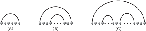
Sparsification is a method tailored to speed up DP-algorithms predicting mfe-secondary structures [spar:07, Backofen:11]. The idea is to prune certain computation paths encountered in the DP-recursions, see Figure . To make the key point, let us consider the case of RNA secondary structure folding. Here sparsification reduces the DP-recursion paths to be based on so called candidates. A candidate is in this case an interval, for which the optimal solution cannot be written as a sum of optimal solutions of sub-intervals, see Figure . Tracing back these candidates gives rise to “irreducible” structures and the crucial observation is here that these irreducibles appear only at a low rate. This means that there are only relatively few candidates, which in turn implies a significant reduction in time and space complexity.
Sparsification has been applied in the context of RNA-RNA interaction structures [Backofen:08] as well as RNA pseudoknot structures [Backofen:10]. In difference to RNA secondary structures, however, not every decomposition rule in the DP-folding of RNA pseudoknot structures is amendable to sparsification. By construction, sparsification can only be applied for calculating mfe-energy structures. Since the computation of the partition function [McCaskill:90, Dirks:03] needs to take into account all sub-structures, sparsification does not work.


For the mfe-folding of RNA secondary structures considerable attention has been paid in order to validate that the set of candidates is small. The idea here is that irreducibles are contained in short, “rainbow”-like arcs. To be precise, the gain is , if secondary structure satisfy the so called polymer-zeta property [Kafri:00, Kabakcioglu:05]: The latter quantifies the probability of an arc of length to be , where , . Note that these arcs confine in case of secondary structures irreducible structures, that is arcs and irreducibility are tightly connected.
In pseudoknotted RNA structures however, we have crossing arcs and the associated notion of irreducible structures differs significantly from that of RNA secondary structures. The polymer-zeta property is theoretically justified by means of modeling the 2D folding of a polymer chain as a self-avoiding walk (SAW) in a 2D lattice [Venderzande:98]. More evidence of the polymer-zeta property for RNA secondary structures has been collected via the NCBI database [NCBI] of mfe-RNA structures.
In this paper we study the sparsification of the decomposition rule that splices an interval [Backofen:10, Backofen:11] in the context of the DP-folding of RNA pseudoknot structures of fixed topological genus. Our paper provides a combinatorial framework to quantify the effects of sparsifying the -decomposition rule.
We shall prove that the candidate set [spar:07, Backofen:10, Backofen:11] is indeed small. Our argument is based on assuming a specific distribution of irreducible structures within mfe-structures. Namely we assume these irreducibles to appear with probability , where we assume to be a fixed parameter and to be a bivariate (energy-filtered) generating function whose associated generation function of irreducibles is .
While this energy-filtration seems to be reparameterization of the notion of “stickiness” [Nebel:03], it is really fundamentally different. This becomes clear when considering loop-based energies which distinguishes energy and arcs. Clearly when folding random sequences one weights the latter around , reminiscent of the probability of two given positions to be compatible. The energy however is fairly independent as it really depends on the particular loop-type.
We obtain these energy-filtered GFs also for RNA pseudoknot structures of fixed topological genus. This provides new insights into the improvements of the sparsification of the concatenation-rule in the presence of cross serial interactions. Our observations complement the detailed analysis of Backofen [Backofen:10, Backofen:11]. We show that although for pseudoknot structures of fixed topological genus [Bon:08, rnag3] the effect of sparsification on the global time complexity is still unclear, the decomposition rule that splits an interval can be sped up significantly.
Sparsification
The general idea of sparsification [spar:07, Backofen:10, Backofen:11] is following: let be a set whose elements are unions of pairwise disjoint intervals. Let furthermore denote an optimal solution (a positive number or score) of the DP-routine over . By assumption is recursively obtained. Suppose the optimal solution is given by , where . Then, under certain circumstances, the DP-routine may interpret either as or as , see Figure . To be precise, this situation is encountered iff
- •
there exists an optimal solution for a sub-structure over where via and is obtained from and via ,
- •
there exists an optimal solution for a sub-structure over where via and is obtained by and via .
Given a decomposition L_v= ⏟ ⏟ L_v_1+L_v_2 _Λ_2+L_v_3 _Λ_1, we call -compatible to if there exists a decomposition rule such that L_v= ⏟ L_v_1+ ⏟ L_v_2+L_v_3 _Λ_3 _Λ_1. Note that if is -compatible to then is -compatible to . To summarize
Definition 1.
(-compatible) Suppose is the optimal solution for over , under decomposition rule . is obtained from two optimal solutions and under rule . Then is called -compatible to if there exist some rule such that and .

Figure depicts two such ways that realize the same optimal solution . Sparsification prunes any such multiple computations of the same optimal value.
We next come to the important concept of candidates. The latter mark the essential computation paths for the DP-routine.
Definition 2.
(Candidates) Suppose is an optimal solution. We call is a -candidate if for any obtained by and , we have
and we shall denote the set of -candidates set by .
Lemma 1.
[spar:07, Backofen:10] Suppose is -compatible to then any optimal solution can be obtained via -candidates.
By construction a -candidate is a union of disjoint intervals such that its optimal solution cannot be obtained via a -splitting. This optimal solution allows to construct a non-unique arc-configuration (sub-structure) over [Zuker:89, Hofacker:94a] and the above -splitting consequently translates into a splitting of this sub-structure. This connects the notion of -candidates with that of sub-structures and shows that a -candidate implies an sub-structure that is -irreducible.
In the case of sparsification of RNA secondary structures we have one basic decomposition rule acting on intervals, namely splices an interval into two disjoint, subsequent intervals. The implied notion of a -irreducible sub-structure is that of a sub-structure nested in an maximal arc, where maximal refers to the partial order iff . This observation relates irreducibility to that or arcs and following this line of thought [spar:07] identifies a specific property of polymer-chains introduced in [Kafri:00, Kabakcioglu:05] to be of relevance for the size of candidate sets:
Definition 3.
(Polymer-zeta property) Let denotes the probability of a structure over an interval under some decomposition rule . Then we say follows the polymer-zeta property if for some constant .
This property is theoretically justified by means of modeling the 2D folding of a polymer chain as a self-avoiding walk (SAW) in a 2D lattice [Venderzande:98].
RNA secondary structures
In this section we recall some results of [spar:07, Backofen:11] on the sparsification of RNA secondary structures. Secondary structure satisfies a simple recursion which gives the optimal solution over by , where denotes the optimal solution in which is a base pair, and denotes the optimal solution obtained by adding the optimal solutions of two subsequent intervals, respectively. Note that the optimal solution over a single vertex is denoted by . We have the recursion equation for and :
where is the score when form a base pair, see Figure. . In case two positions, , in the sequence are incompatible then we have .

An interval is a -candidate if the optimal solution over is given by . Indeed, is a candidate iff is in the candidate set of , and we denote the set by . Suppose the optimal solution is given by and suppose we have . Then since is not a candidate, Lemma shows that we can compute , where is a candidate.
Accordingly, the recursion for can be based on candidates, i.e. . Clearly, the bottleneck for computing the recursion is the calculation of , which requires time. Applying sparsification, this recursion is based on candidates . Suppose we have such candidates, then the time complexity reduces to , since the optimal solution is necessarily based on a candidate. Once the latter is identified the expression requires only time complexity. In the worst case, contains elements.
The polymer-zeta property however implies that the expectation of is given by where and are constants and . We can conclude from the polymer-zeta property that and accordingly the runtime reduces to .
RNA pseudoknot structures
Sparsification can also be applied to the DP-algorithm folding RNA structures with pseudoknots [Backofen:10]. In contrast to the decomposition rule that spliced an interval into two subsequent intervals, we encounter in the grammar for pseudoknotted structures additional more complex decomposition rules [Rivas:99]. As shown in [Backofen:10] there exist some decomposition rules which are not -compatible and which can accordingly not be sparsified at all, see Figure . For instance, given a decomposition rule in pknot-R&E subsequent decomposition rules which are -compatible to are referred to as split type of [Backofen:10].
In the following we will study RNA pseudoknot structures of fixed topological genus, see Section Diagrams, surfaces and some generating functions for details. An algorithm folding such pseudoknot structures, gfold, has been presented in [Reidys:11a]. The decomposition rules that appear in gfold are reminiscent to those of pknot-R&E but as they restrict the genus of sub-structures the iteration of gap-matrices is severely restricted and the effect of sparsification of these decompositions is significantly smaller.

In the following, we restrict our analysis to the decomposition rule which splices an interval into two subsequent intervals. Expressed in combinatorial language, cuts the backbone of an RNA pseudoknot structure of fixed genus over one interval without cutting a bond.
Methods
Diagrams and genus filtration
In this section we recall some facts about diagrams and pass from diagrams to surfaces in order to be able to formulate what we mean by an RNA pseudoknot structure of fixed genus . Most of this section is derived from [Zagier:95, rnag3] with the exception of Lemma and Theorem , which are new and key for the subsequent analysis of -candidates.
A diagram is a labeled graph over the vertex set in which each vertex has degree , represented by drawing its vertices in a horizontal line. The backbone of a diagram is the sequence of consecutive integers together with the edges . The arcs of a diagram, , where , are drawn in the upper half-plane. We shall distinguish the backbone edge from the arc , which we refer to as a -arc. A stack of length is a maximal sequence of “parallel” arcs, and is also referred to as a -stack, see Figure .

We shall consider diagrams as fatgraphs, , that is graphs together with a collection of cyclic orderings, called fattenings, one such ordering on the half-edges incident on each vertex. Each fatgraph determines an oriented surface [Loebl:08, Penner:10] which is connected if is and has some associated genus and number of boundary components. Clearly, contains as a deformation retract [Massey:69]. Fatgraphs were first applied to RNA secondary structures in [Waterman:93] and [Penner:03].
A diagram hence determines a unique surface (with boundary). Filling the boundary components with discs we can pass from to a surface without boundary. Euler characteristic, , and genus, , of this surface is given by and , respectively, where is the number of discs, ribbons and boundary components in , [Massey:69]. The genus of a diagram is that of its associated surface without boundary and a diagram of genus is referred to as -diagram.
A -diagram without arcs of the form (-arcs) is called a -structure. A -diagram that contains only vertices of degree three, i.e. does not contain any vertices not incident to arcs in the upper halfplane, is called a -matching. A stack of length is a maximal sequence of “parallel” arcs, ((i,j),(i+1,j-1),…,(i+τ,j-τ)).
A diagram is called irreducible, if and only if it cannot be split into two by cutting the backbone without cutting an arc.
Let and denote the number of -matchings and -structures having -arcs and vertices, respectively, with GF C_g(z)=∑_n=0^∞c_g(n)z^n D_g(z)= ∑_n=0^∞d_g(n)z^n. The GF has been computed the context of the virtual Euler characteristic of the moduli-space of curves in [Zagier:95] and can be derived from by means of symbolic enumeration [rnag3]. The GF of genus zero diagrams is wellknown to be the GF of the Catalan numbers, i.e., the numbers of triangulations of a polygon with sides, C_0(z)= 1- 1-4z 2z . As for we have the following situation [rnag3]
Theorem 1.
Suppose . Then the following assertions hold
(a) is algebraic and
| (1) |
In particular, we have for some constant depending only on and :
| (2) |
(b) the bivariate GF of -structures over vertices, containing exactly arcs, , is given by
| (3) |
Irreducible -structures
In the context of -candidates we observed that irreducible substructures are of key importance. It is accordingly of relevance to understand the combinatorics of these structures. To this end let denote the GF of irreducible -structures.
Lemma 2.
For , the GF satisfies the recursion
For a proof of Lemma , see Section Proofs.
Theorem 2.
For we have
(a) the GF of irreducible -structures over
vertices is given by
| (4) |
where , and are both polynomials with lowest degree at least , and , . In particular, for some constant and :
| (5) |
(b) the bivariate GF of irreducible -structures over vertices, containing exactly arcs, , is given by
| (6) |
where .
We shall postpone the proof of Theorem to Section Proofs.
The main result
In Section Sparsification we observed that sparsification applies to the decomposition rule , which effectively splices off an irreducible sub-structure (diagram). This notion of -irreducibility is indeed compatible by the notion of combinatorial irreducibility introduced in Section Diagrams, surfaces and some generating functions, see Figure . An optimal solution for the original structure is obtained from an optimal solution of the spliced, -irreducible, sub-structure and an optimal solution for the remaining sub-structure.

Folded configurations are energetically optimal and dominated by the stacking of adjacent base pairs [Mathews:99], as well as minimum arc-length conditions [Waterman:78aa] discussed before.
In the following we mimic some form of minimum free energy -structures: inspired by the Nussinov energy model [Nussinov:78] we consider the weight of a -structure over vertices to be given by , where is the number of arcs for some [Nebel:03]. Note that the case corresponds to the uniform distribution, i.e. all -structure have identical weight.
This approach requires to keep track of the number of arcs, i.e. we need to employ bivariate GF. In Theorem (b) we computed this bivariate GF and in Theorem (b) we derived from this bivariate GF , the GF of irreducible -structures over vertices containing arcs.
The idea now is to substitute for the second indeterminant, , some fixed . This substitution induces the formal power series D_g,η(z)=E_g(z,η), which we regard as being parameterized by . Obviously, setting we recover , i.e. we have . Note that for , the polynomial has no real root. Thus we have for the asymptotics
| (7) |
with identical exponential growth rates as long as the supercritical paradigm [Flajolet:07a] applies, i.e. as long as , the real root of minimal modulus of ( η z 2 (η z 2 -z+1) 2 )= 1 4 , is smaller than any singularity of . In this situation affects the constant and the exponential growth rate but not the sub-exponential factor . The latter stems from the singular expansion of . Analogously, we derive the -parameterized family of GF . Assuming a random sequence has on average a probability at most to form a base pair we fix in the following , where is the Euler number. By abuse of notation we will omit the subscript assuming .
The main result of this section is that the set of -candidates is small. To put this size into context we note that the total number of entries considered for the -decomposition rule is given by Ω(n)=∑_m=1^n(n-m+1).
Theorem 3.
Suppose an mfe -structure over an interval of length is irreducible with probability , then the expected number of candidates of -structures for sequences of lengths satisfies
and furthermore, setting we have
where is a constant.
We provide an illustration of Theorem in Figure .

Proof.
We proof the theorem by quantifying the probability of being a -candidate. In this case any (not necessarily unique) sub-structure, realizing the optimal solution , is -irreducible, and therefore an irreducible structure over .
Let , by assumption, the probability that is a candidate conditional to the existence of a substructure over is given by
| (8) |
Note that does not depend on the relative location of the interval but only on the interval-length. Let , then according to Theorem ,
for where and are constants. On the one hand
| (9) |
where is a constant. On the other hand, we have
| (10) |
Setting , we can conclude that , see Fig. .

We next study the expected number of candidates over an interval of length . To this end let X_m= —{[i,j]∣[i,j] is a -candidate of length }—. The expected cardinality of the set of -candidates of length encountered in the DP-algorithm is given by
since there are starting points for such an interval . Therefore, by linearity of expectation, for sufficiently large , with being a small constant. Thus we have
| (11) |
Consequently, the expected size of the -candidate set is . We proceed by comparing the expected number of candidates of a sequence with length with ,
For sufficient large , . Furthermore
from which we can conclude and the theorem is proved. ∎
Loop-based energies
In this section we discuss the more realistic loop-based energy model of RNA secondary structure folding. To be precise we evoke here instead of two trivariate GFs and counting secondary structures over vertices that filter energy and arcs.
This becomes necessary since the loop-based model distinguishes between arcs and energy. The “cancelation” effect or reparameterization of stickiness [Nebel:03] to which we referred to before does not appear in this context. Thus we need both an arc- as well as an energy-filtration.
A further complication emerges. In difference to the GFs and the new GFs are not simply obtained by formally substituting into the power series and as bivariate terms. The more complicated energy model requires a specific recursion for irreducible secondary structures.
The energy model used in prediction secondary structure is more complicated than the simple arc-based energy model. Loops which are formed by arcs as well as isolated vertexes between the arcs are considered to give energy contribution. Loops are categorized as hairpin loops (no nested arcs), interior loops (including bulge loops and stacks) and multi-loops (more than two arc nested), see Figure . An arbitrary secondary structure can be uniquely decomposed into a collection of mutually disjoint loops. A result of the particular energy parameters [Mathews:99] is that the energy model prefers interior loops, in particular stacks (no isolated vertex between two parallel arc), and disfavors multi-loops. Base on this observation, we give a simplified energy model for a loop contained in secondary structure by
- •
if is a hairpin loop,
- •
if is an interior loop,
- •
if is a multi-loop,
where is a loop. The weight for a secondary structure accordingly is given by
| (12) |
Let and be the GFs obtained by setting and in and , where is the Euler number. This means we find a suitable parameterization which brings us back to a simple univariate GF.
Lemma 3.
The weight function of RNA secondary structures, , satisfies
| (13) |
and is uniquely determined by the above equation. Furthermore
| (14) |
Proof.
We first consider the GF whose coefficient of denotes the total weight of irreducible secondary structures over vertexes, where is an arc. Thus it gives a term . Isolated vertex lead to the term z^p ∑_i=0^∞ z^i=z^p 1 1-z , where denotes the minimum number of isolated vertexes to be inserted. Depending on the types of loops formed by , we have
- •
hairpin loops: ,
- •
interior loops: ,
- •
multi-loops: there are at least two irreducible substructures, as well as isolated vertices, thus
We compute F^*_0(z)= 6 16 (e^0.5 z^2 z 1-z +e^1 z^2 ( 1 1-z )^2 F^*_0(z)+e^-5 z^2 ( F 0 * (z) 1 1-z ) 2 1-F 0 * (z) 1 1-z 1 1-z ), which establishes the recursion. The uniqueness of the solution as a power series follows from the fact that each coefficient can evidently be recursively computed.
An arbitrary secondary structure can be considered as a sequence of irreducible substructure with certain intervals of isolated vertexes. Thus F_0(z)= 1 1-z ∑_i=0^∞ 1 1-z F^*_0(z)= 1 1-z 1 1-F 0 * (z) 1 1-z . ∎
Lemma 4.
and have the same singular expansion.
| (15) |
where and are constants and
Proof.
Solving eq. we obtain a unique solution for whose coefficient are all positive. Observing the dominant singularity of it is . is a function of and we examine the real root of minimal modulus of is bigger than . Then by the supercritical paradigm [Flajolet:07a] applying, and have identical exponential growth rates. Furthermore, and have the same sub-exponential factor , hence the lemma. ∎
Theorem 4.
Suppose an mfe secondary structure over an interval of length is irreducible with probability , then the expected number of candidates for sequences of lengths is
and furthermore, setting , we have
where .
Proof.
By Lemma we have where is a constant. The proof is completely analogous to that of Theorem . ∎
We show the distribution of and in Figure .

Results and Discussion
In this paper we quantify the effect of sparsification of the particular decomposition rule . This rule splits and interval and thereby separates concatenated substructures. The sparsification of alone is claimed to provide a speed up of up to a linear factor of the DP-folding of RNA secondary structures [spar:07]. A similar conclusion is drawn in [Backofen:08] where the sparsification of RNA-RNA interaction structures is shown to experience also a linear reduction in time complexity. Both papers [spar:07, Backofen:08] base their conclusion on the validity of the polymer-zeta property discussed in Section Sparsification.
For the folding of pseudoknot structures there may however exist non-sparsifiable rules in which case the overall time complexity is not reduced. The key object here is the set of candidates and we provide an analysis of -candidates by combinatorial means. In general, the connection between candidates, i.e. unions of disjoint intervals and the combinatorics of structures is actually established by the algorithm itself via backtracking: at the end of the DP-algorithm a structure is being generated that realizes the previously computed energy as mfe-structure. This connects intervals and sub-structures.
So, does polymer-zeta apply in the context of RNA structures? In fact polymer-zeta would follow if the intervals in question are distributed as in uniformly sampled structures. This however, is far from reasonable, due to the fact that the mfe-algorithm deliberately designs some mfe structure over the given interval. What the algorithm produces is in fact antagonistic to uniform sampling. We here wish to acknowledge the help of one anonymous referee in clarifying this point.
Our results clearly show that the polymer-zeta property, i.e. the probability of an irreducible structure over an interval of length satisfies a formula of the form
| (16) |
does not apply for RNA structures. The theoretical findings from self-avoiding walks [Kabakcioglu:05] unfortunately do not allow to quantify the expected number of candidates of the -rule in RNA folding.
That the polymer-zeta property does not hold for RNA has also been observed in the context of the limit distribution of the 5’-3’ distances of RNA secondary structures [Hillary:11]. Here it is observed that long arcs, to be precise arcs of lengths always exist. This is of course a contradiction to eq. ().
The key to quantification of the expected number of candidates is the singularity analysis of a pair of energy-filtered GF, namely that of a class of structures and that of the subclass of all such structures that are irreducible. We show that for various energy models the singular expansions of both these functions are essentially equal–modulo some constant. This implies that the expected number of candidates is and all constants can explicitly be computed from a detailed singularity analysis. The good news is that depending on the energy model, a significant constant reduction, around can be obtained. This is in accordance with data produced in [Backofen:11] for the mfe-folding of random sequences. There a reduction by is reported for sequences of length .
Our findings are of relevance for numerous results, that are formulated in terms of sizes of candidate sets [Backofen:10]. These can now be quantified. It is certainly of interest to devise a full fledged analysis of the loop-based energy model. While these computations are far from easy our framework shows how to perform such an analysis.
Using the paradigm of gap-matrices Backofen has shown [Backofen:10] that the sparsification of the DP-folding of RNA pseudoknot structures exhibits additional instances, where sparsification can be applied, see Fig. (B). Our results show that the expected number of candidates is , where the constant reduction is around . This is in fact very good new since the sequence length in the context of RNA pseudoknot structure folding is in the order of hundreds of nucleotides. So sparsification of further instances does have an significant impact on the time complexity of the folding.
Proofs
In this section, we prove Lemma and Theorem .
Proof for Lemma : let and be the bivariate GF , and . Suppose a structure contains exactly irreducible structures, then
| (17) |
and
| (18) |
as well as . Let . Then , whence for ,
| (19) |
and , where . Furthermore, we have and
| (20) |
which implies and
| (21) |
Proof for Theorem
Let denotes the set of compositions of having parts,
i.e. for we have
and .
Claim.
| (22) |
We shall prove the claim by induction on . For we have
| (23) |
whence eq. () holds for . By induction hypothesis, we may now assume that for , eq. () holds. According to Lemma , we have
We next observe
| (24) |
and setting we obtain,
and setting
Consequently, the Claim holds for any .
For any , we have [rnag3] D_g(z) = 1 z 2 -z+1 P g (u) (1-4u) 3g-1/2 , D_0(z) = 1 z 2 -z+1
