Alternating Linearization for Structured Regularization Problems
Abstract
We adapt the alternating linearization method for proximal decomposition to structured regularization problems, in particular, to the generalized lasso problems. The method is related to two well-known operator splitting methods, the Douglas–Rachford and the Peaceman–Rachford method, but it has descent properties with respect to the objective function. This is achieved by employing a special update test, which decides whether it is beneficial to make a Peaceman–Rachford step, any of the two possible Douglas–Rachford steps, or none. The convergence mechanism of the method is related to that of bundle methods of nonsmooth optimization. We also discuss implementation for very large problems, with the use of specialized algorithms and sparse data structures. Finally, we present numerical results for several synthetic and real-world examples, including a three-dimensional fused lasso problem, which illustrate the scalability, efficacy, and accuracy of the method.
keywords
Lasso, Fused Lasso, Nonsmooth Optimization, Operator Splitting1 Introduction
Regularization techniques that encourage sparsity in parameter estimation have gained increasing popularity recently. The most widely used example is lasso (Tibshirani, 1996), where the loss function is penalized by the -norm of the unknown coefficients , to form a modified objective function,
| (1) |
in order to shrink irrelevant coefficients to zero. Many efficient algorithms have been proposed to solve this problem, including (Fu, 1998; Daubechies et al., 2004; Efron et al., 2004) and (Friedman et al., 2007). Some of them are capable of handling massive data sets with tens of thousands of variables and observations.
For many practical applications, physical constraints and domain knowledge may mandate additional structural constraints on the parameters. For example, in cancer research, it may be important to consider groups of interacting genes in each pathway rather than individual genes. In image analysis, it is natural to regulate the differences between neighboring pixels in order to achieve smoothness and reduce noise. In light of these popular demands, a variety of structured penalties have been proposed to incorporate prior information regarding model parameters. One of the most important structural penalties is the fused lasso proposed in (Tibshirani et al., 2005). It utilizes the natural ordering of input variables to achieve parsimonious parameter estimation on neighboring coefficients. Chen et al. (2010) developed the graph induced fused lasso that penalizes differences between coefficients associated with nodes in a graph that are connected. Beck and Teboulle (2009) proposed the total variation penalty for image denoising and deblurring, in a similar fashion to the two-dimensional fused lasso. Similar penalty functions have been successfully applied to several neuroimaging studies (Michel et al., 2011; Grosenick et al., 2011; Grosenick et al., 2013). More recently, Zhang et al. (2012) applied a generalized version of fused lasso to reconstruct gene copy number variant regions. A general structural lasso framework was proposed in (Tibshirani and Taylor, 2011), with the following form:
| (2) |
where is an matrix that defines the structural constraints one wants to impose on the coefficients. Many regularization problems, including high dimensional fused lasso and graph induced fused lasso, can be cast in this framework.
When the structural matrix is relatively simple, as in the original lasso case with , traditional path algorithms and coordinate descent techniques can be used to solve the optimization problems efficiently (Friedman et al., 2007). For more complex structural regularization, these methods cannot be directly applied. One of the key difficulties is the non-separability of the nonsmooth penalty function. Coordinate descent methods fail to converge under this circumstances (Tseng, 2001). Generic solvers, such as interior point methods, can sometimes be used; unfortunately they become increasingly inefficient for large size problems, particularly when the design matrix is ill-conditioned (Chen et al., 2012).
In the past two years, many efforts have been devoted to developing efficient optimization techniques for solving regularization problems using structured penalties. Liu et al. (2010) and Ye and Xie (2011) developed a first-order and a split Bregman scheme, respectively, for solving similar class of problems. Chen et al. (2012) proposed a modified proximal technique for the general structurally penalized problems. It is based on a first order approximation of the nonsmooth penalty function, which can become unstable when dimension is high. Meanwhile, several path algorithms have also been proposed to compute the whole regularization path for the general fused lasso problem. Hoefling (2010) developed a path algorithm for solving (2) when the matrix is nonsingular. This technique is not applicable to cases with large dimension of and small number of observations, such as gene expression and brain imaging analysis. Tibshirani and Taylor (2011) extended the path algorithm to include all design matrices , by computing the regularization path of the dual problem. Although fairly general, this version of the path algorithm does not scale well with data dimension, as the knots of the piecewise linear solution path become very dense. Many of the proposed approaches are versions of the operator splitting methods or their dual versions, alternating direction methods (see, e.g., Boyd et al. (2010); Combettes and J.-C. (2011), and the references therein). Although fairly general and universal, they frequently suffer from slow tail convergence (see (He and Yuan, 2011) and the references therein).
Thus, a need arises to develop a general approach that can solve large scale structured regularization problem efficiently. For such an approach to be successful in practice, it should guarantee to converge at a fast rate, be able to handle massive data sets, and should not rely on approximating the penalty function. In this paper, we propose a framework based on the alternating linearization algorithm of (Kiwiel et al., 1999), that satisfies all these requirements.
We consider the following generalization of (2):
| (3) |
where is a norm in . Our considerations and techniques will apply to several possible choices of this norm, in particular, to the norm , and to the total variation norm used in image processing.
Formally, we write the objective function as a sum of two convex functions,
| (4) |
where is a loss function, which is assumed to be convex with respect to , and is a convex penalty function. Any of the functions (or both) may be nonsmooth, but an essential requirement of our framework is that each of them can be easily minimized with respect to , when augmented by a separable linear-quadratic term , with some vectors , . Our method bears resemblance to operator splitting and alternating direction approaches, but differs from them in the fact that it is monotonic with respect to the values of (4). We discuss these relations and differences later in section 2.2, but roughly speaking, a special test applied at every iteration of the method decides which of the operator splitting iterations is the most beneficial one.
In our applications, we focus on the quadratic loss function and the penalty function in the form of generalized lasso (3), as the most important case, where comparison with other approaches is available. This case satisfies the requirement specified above, and allows for substantial specialization and acceleration of the general framework of alternating linearization. In fact, it will be clear from our presentation that any convex loss function can be handled in exactly the same way.
An important feature of our approach is that problems with the identity design matrix are solved exactly in one iteration, even for very large dimension.
The remainder of the paper is organized as follows. In Section 2, we introduce the alternating linearization method and we discuss its relations to other approaches. Section 3 briefly discusses the application to lasso problems. In section 4 we describe the application to general structured regularization problems. Section 5 presents simulation results and real data examples, which illustrate the efficacy, accuracy, and scalability of the alternating linearization method. Concluding remarks are presented in section 6. The appendix contains details about the algorithms used to solve the subproblems of the alternating linearization method.
2 The alternating linearization method
2.1 Outline of the method
In this section, we describe the alternating linearization (ALIN) approach to minimize (4). It is an iterative method, which generates a sequence of approximations converging to a solution of the original problem (4), and two auxiliary sequences: and , where is the iteration number. Each iteration of the ALIN algorithm consists of solving two subproblems: the -subproblem and the -subproblem, and of an update step, applied after any of the subproblems, or after each of them.
At the beginning we set , where is the starting point of the method. In the description below, we suppress the superscript denoting the iteration number, to simplify notation.
The -subproblem
We linearize at , and approximate it by the function
If is differentiable, then ; for a general convex , we select a subgradient . In the first iteration, this may be an arbitrary subgradient; at later iterations special selection rules apply, as described in (8) below.
The approximation is used in the optimization problem
| (5) |
in which the last term is defined as follows:
with a diagonal matrix , , . The solution of the -subproblem (5) is denoted by .
We complete this stage by calculating the subgradient of at , which features in the optimality condition for the minimum in (5):
Elementary calculation yields the right subgradient :
| (6) |
The -subproblem
Using the subgradient we construct a linear minorant of the penalty function as follows:
This approximation is employed in the optimization problem
| (7) |
The optimal solution of this problem is denoted by . It will be used in the next iteration as the point at which the new linearization of will be constructed. The next subgradient of to be used in the -subproblem will be
| (8) |
The update step
The update step can be applied after any of the subproblems, or after both of them. It changes the current best approximation of the solution , if certain improvement conditions are satisfied. It uses a parameter . In the implementation, we use . The choice of this parameter does not influence the overall performance of the algorithm. We describe it here for the case of applying the update step after the -subproblem; analogous operations are carried out if the update step is applied after the -subproblem.
At the beginning of the update step the stopping criterion is verified. If
| (9) |
the algorithm terminates. Here is the stopping test parameter.
If the the stopping test is not satisfied, we check the inequality
| (10) |
If it is satisfied, then we update ; otherwise remains unchanged.
If the update step is applied after the -subproblem, we use instead if in the inequalities (9) and (10).
The update step is a crucial component of the alternating linearization algorithm; it guarantees that the sequence is monotonic, and it stabilizes the entire algorithm (see the remarks at the end of section 5.2). It is a specialized form of the main distinction between null and serious steps in bundle methods for nonsmooth optimization. The Reader may consult the books Bonnans et al. (2003); Hiriart-Urruty and Lemaréchal (1993); Kiwiel (1985); Ruszczyński (2006) and the references therein for the theory of bundle methods and the significance of null and serious steps in these methods.
2.2 Relation to operator splitting and alternating direction methods
Our approach is intimately related to operator splitting methods and their dual versions, alternating direction methods, which are recently very popular in the area of signal processing (see, e.g., (Boyd et al., 2010; Combettes and J.-C., 2011; Fadili and Peyré, 2011)). To discuss these relations, it is convenient to present our method formally, and to introduce two running proximal centers:
After elementary manipulations we can absorb the linear terms into the quadratic terms and summarize the alternating linearization method as follows.
The Update Test in lines 3 and 8 is the corresponding version of inequality (10). The Stopping Test is inequality (9).
If we assume that the update steps in lines 4 and 9 are carried out after every -subproblem and every -subproblem, without verifying the update test (10), then the method becomes equivalent to a scaled version of the Peaceman–Rachford algorithm (originally proposed by (Peaceman and Rachford, 1955) for PDEs and later generalized and analyzed by (Lions and Mercier, 1979); see also (Combettes, 2009) and the references therein). If with , then we obtain an unscaled version of this algorithm.
If we assume that the update steps are carried out after every -subproblem without verifying inequality (10), but never after -subproblems, then the method becomes equivalent to a scaled version of the Douglas–Rachford algorithm (introduced by (Douglas and Rachford, 1956), and generalized and analyzed by (Lions and Mercier, 1979); see also (Bauschke and Combettes, 2011) and the references therein). As the roles of and can be switched, the method in which updates are carried always after -subproblems, but never after -subproblems, is also equivalent to a scaled Douglas–Rachford method.
Operator splitting methods are not monotonic with respect to the values of the objective function . Their convergence is based on monotonicity with respect to the distance to the optimal solution of the problem (Lions and Mercier, 1979; Eckstein and Bertsekas, 1992).
In contrast, the convergence mechanism of our method is different; it draws from some ideas of bundle methods in nonsmooth optimization (Hiriart-Urruty and Lemaréchal, 1993; Kiwiel, 1985; Ruszczyński, 2006). Its key element is the update test employed in (10). At every iteration we decide whether it is beneficial to make a Peaceman–Rachford step, any of the two possible Douglas–Rachford steps, or none. In the latter case, which we call the null step, remains unchanged, but the trial points and are updated. These updates continue, until or become better than , or until optimality is detected (cf. the remarks at the end of section 5.2). In may be worth noticing that the recent application of the idea of alternating linearization in Goldfarb et al. (2013) removes the update test from the method of Kiwiel et al. (1999), thus effectively reducing it to an operator splitting method.
Alternating direction methods are dual versions of the operator splitting methods, applied to the following equivalent form of the problem of minimizing (4):
| (11) |
In regularized signal processing problems, when with some fixed matrix , the convenient problem formulation is
The dual functional,
has the form of a sum of two functions, and the operator splitting methods apply. The reader may consult (Boyd et al., 2010; Combettes and J.-C., 2011) for appropriate derivations. It is also worth mentioning that the alternating direction methods are sometimes called split Bregman methods in the signal processing literature (see, e.g., (Goldstein and Osher, 2009; Ye and Xie, 2011), and the references therein). Recently, (Qin and Goldfarb, 2012) applied alternating direction methods to some structured regularization problems resulting from group lasso models.
However, to apply our alternating linearization method to the dual problem of maximizing , we would have to be able to quickly compute the value of the dual functions, in order to verify the update condition (10), as discussed in detail in Kiwiel et al. (1999). The second dual function, is rather difficult to evaluate, and it makes the update test time consuming. Without this test, our method reduces to the alternating direction method, which does not have descent properties, and whose tail convergence may be slow. Our experiments reported at the end of section 5.2 confirm these observations.
2.3 Convergence
Convergence properties of the alternating linearization method follow from the general theory developed in (Kiwiel et al., 1999). Indeed, after the change of variables we see that the method is identical to Algorithm 3.1 of (Kiwiel et al., 1999), with . The following statement is a direct consequence of (Kiwiel et al., 1999, Theorem 4.8).
Theorem 1.
For structured regularization problems the assumption of the theorem is satisfied, because both the loss function and the regularizing function are bounded from below, and one of the purposes of the regularization term is to make the set of minima of the function nonempty and bounded.
It may be of interest to look closer at the stopping test (9) employed in the update step.
Lemma 2.
Suppose is the unique minimum point of and let be such that for all . Then the stopping criterion (9) implies that
| (12) |
Proof.
As , inequality (9) implies that
| (13) | ||||
The expression on the left hand side of this inequality is the Moreau–Yosida regularization of the function evaluated at . By virtue of (Ruszczyński, 2006, Lemma 7.12), after setting and with the norm , the Moreau–Yosida regularization satisfies the following inequality:
Combining this inequality with (13) and simplifying, we conclude that
Substitution of the denominator by the upper estimate yields (12). ∎
If is unique then grows at least quadratically in the neighborhood of . This implies that satisfying the assumptions of Lemma 2 exists. Our use of the norm amounts to comparing the function to its diagonal approximation for . The reader may also consult (Ruszczyński, 1995, Lemma 1) for the accuracy of the diagonal approximation when the matrix is sparse.
If the original problem is to minimize (4) subject to the constraint that for some convex closed set , we can formally add the indicator function of this set,
to or to (whichever is more convenient). This will result in including the constraint in one of the subproblems, and changing the subgradients accordingly. The theory of Kiwiel et al. (1999) covers this case as well, and Theorem 1 remains valid.
3 Application to lasso regression
First, we demonstrate the alternating linearization algorithm (ALIN) on the classical lasso regression problem. Due to the separable nature of the penalty function, very efficient coordinate descent methods are applicable to this problem as well (Tseng, 2001), but we wish to illustrate our approach on the simplest case first.
In the lasso regression problem we have
where is the design matrix, is the vector of response variables, is the vector of regression coefficients, and is a parameter of the model.
We found it essential to use , that is, , . This choice is related to the diagonal quadratic approximation of the function , which was employed (for similar objectives in the context of augmented Lagrangian minimization) by Ruszczyński (1995). Indeed, in the -subproblem in the formula (14) below, the quadratic regularization term is a quadratic form built on the diagonal of the Hessian of .
The -subproblem
The -subproblem
The problem (7), after skipping constants, simplifies to the unconstrained quadratic programming problem
| (16) |
Its solution can be obtained by solving the following symmetric linear system in :
| (17) |
This system can be efficiently solved by the preconditioned conjugate gradient method (see, e.g., (Golub and Van Loan, 1996)), with the diagonal preconditioner . Its application does not require the explicit form of the matrix ; only matrix-vector multiplications with and are employed, and they can be implemented with sparse data structures.
The numerical accuracy of this approach is due to the good condition index of the resulting matrix, as explained in the following lemma.
Lemma 3.
The application of the preconditioned conjugate gradient method with preconditioner to the system (17) is equivalent to the application of the conjugate gradient method to a system with a symmetric positive definite matrix whose condition index is at most .
Proof.
By construction, the preconditioned conjugate gradient method with a preconditioner applied to a system with a matrix is the standard conjugate gradient method applied to a system with the matrix . Substituting the matrix from (17), we obtain:
Define . By the construction of , all columns , , of have Euclidean length 1.
The condition index of is equal to
As the matrix is positive semidefinite, . To estimate suppose is the corresponding eigenvector of Euclidean length 1. We obtain the chain of relations:
Therefore, the condition index of is at most . ∎
4 Application to general structured regularization problems
In the following we apply the alternating linearization algorithm to solve more general structured regularization problems including the generalized Lasso (3). Here we assume the least square loss, as in the previous subsection. The objective function can be written as follows:
| (18) |
For example, for the one-dimensional fused lasso, is the following matrix:
and the norm is the -norm , but our derivations are valid for any form of , and any norm .
The -subproblem
The -subproblem can be equivalently formulated as follows:
| (19) |
Owing to the use of , and with , it is a quite accurate approximation of the original problem, especially for sparse (Ruszczyński, 1995).
The Lagrangian of problem (19) has the form
where is the dual variable. Consider the dual norm , defined as follows:
| (20) |
We see that the minimum of the Lagrangian with respect to is finite if and only if (Ruszczyński, 2006, Example 2.94). Under this condition, the minimum value of the -terms is zero and we can eliminate them from the Lagrangian. We arrive to its reduced form,
| (21) |
To calculate the dual function, we minimize over . After elementary calculations, we obtain the solution
| (22) |
Substituting it back to (21), we arrive to the following dual problem:
| (23) |
This is a norm-constrained optimization problem. Its objective function is quadratic, and the specific form of the constraints depends on the norm used in the regularizing term of (3).
The case of the -norm
If the norm is the -norm , then the dual norm is the -norm:
In this case (23) becomes a box-constrained quadratic programming problem, for which many efficient algorithms are available. One possibility is the active-set box-constrained preconditioned conjugate gradient algorithm with spectral projected gradients, as described in (Birgin and Martínez, 2002; Friedlander and Martínez, 1994). It should be stressed that its application does not require the explicit form of the matrix ; only matrix-vector multiplications with and are employed, and they can be implemented with sparse data structures.
An even better possibility, due to the separable form of the constraints, is coordinate-wise optimization (see, e.g., (Ruszczyński, 2006, Sec. 5.8.2)) in the dual problem (23). In our experiments, the dual coordinate-wise optimization method strictly outperforms the box-constrained algorithm, in terms of the solution time.
The solution of the dual problem can be substituted into (22) to obtain the primal solution.
The case of a sum of -norms
Another important case arises when the vector is split into subvectors , and
| (24) |
This is the group lasso model, also referred to as the -norm regularization (see, e.g. Qin and Goldfarb (2012)). A special case of it is the total variation norm is discussed in section 5.4.
We can directly verify that the dual norm has the following form:
It follows that problem (23) is a block-quadratically constrained quadratic optimization problem:
| (25) | ||||
This problem can be very efficiently solved by a cyclical block-wise optimization with respect to the subvectors . At each iteration of the method, optimization with respect to the corresponding subvector is performed, subject to one constraint . The other subvectors, , are kept fixed on their last values. After that, is incremented (if ) or reset to 1 (if ), and the iteration continues. The method stops when no significant improvements over steps can be observed. The dual block optimization method performs well in the applications we are interested in. General convergence theory can be found in (Tseng, 2001).
Again, the solution of the dual problem is substituted into (22) to obtain the primal solution.
The -subproblem
We obtain the update by solving the linear equation system (17), exactly as in the lasso case.
The special case of
If the design matrix in (18), then our method solves the problem in one iteration, when started from . Indeed, in this case we have , , and the first -subproblem becomes equivalent to the original problem (18):
| (26) |
The dual problem (23) simplifies as follows:
| (27) |
It can be solved by the same block-wise optimization method, as in the general case. The optimal primal solution is then .
5 Numerical experiments
In this section, we present results on a number of simulations and real data studies involving a variety of non-differentiable penalty functions. We compare the alternating linearization algorithm (ALIN) with competing approaches in terms of iteration steps, computation time, and estimation accuracy. All these studies are performed on an AMD 2.6GHZ, 4GB RAM computer using MATLAB.
5.1 regularization
In this section, we compare ALIN with some competing methods for solving the regularization problem:
| (28) |
The methods that we are comparing with are: SpaRSA, a type of iterative thresholding method, considered the best method among its variations; FISTA, a variation of the Nesterov method, considered to be state-of-the-art among the first order methods; and SPG, a spectral gradient method. We follow the procedure described by (Wright et al., 2009) to generate a data set for comparisons. The elements of the matrix are generated independently using a Gaussian distribution with mean zero and variance . The dimension of is by , , and . The true signal, , is a vector with randomly placed spikes and zeros elsewhere. The dependent variables are , where is Gaussian noise with variance .
To make a fair comparison between the methods, we run FISTA on each instance of the problem. FISTA is set to run to or iterations, whichever comes first. Then ALIN, SpaRSA, and SPG are set to run until the objective function values obtained are as good as that of FISTA. We set a parameter and chose values of =, , , and . We allow SpaRSA to run its monotone and continuation feature. Continuation is a special feature of SpaRSA for cases when the parameter is small. With this feature, SpaRSA computes the solutions for bigger values of and uses them to find solutions for smaller values of . We did not let SpaRSA use its special feature de-bias since it involves removing zero coefficients to reduce the size of the data set. This feature makes it unfair for the other competing methods. In Table 1, we report the average time elapsed (in seconds) and the standard deviation after runs.
| ALIN | 17.99 | (10.68) | 36.60 | (15.08) | 105.14 | (40.88) | |
|---|---|---|---|---|---|---|---|
| FISTA | 8.58 | (4.00) | 18.63 | (9.35) | 58.73 | (42.01) | |
| SPARSA | 8.18 | (2.34) | 8.18 | (3.80) | 34.23 | (49.55) | |
| SPG | 160.72 | (27.48) | 160.72 | (47.82) | 404.59 | (79.62) | |
| ALIN | 9.35 | (2.99) | 34.01 | (15.18) | 74.06 | (34.27) | |
| FISTA | 16.91 | (4.57) | 36.43 | (16.66) | 131.91 | (33.94) | |
| SPARSA | 20.55 | (10.08) | 36.81 | (19.29) | 169.88 | (73.01) | |
| SPG | 136.26 | (23.30) | 186.94 | (46.56) | 460.71 | (38.93) | |
| ALIN | 6.30 | (2.73) | 21.83 | (10.17) | 65.79 | (39.49) | |
| FISTA | 18.88 | (2.95) | 48.37 | (15.77) | 158.73 | (21.86) | |
| SPARSA | 35.56 | (11.32) | 74.66 | (24.49) | 234.75 | (64.67) | |
| SPG | 140.00 | (23.15) | 190.43 | (45.48) | 473.78 | (6.41) | |
| ALIN | 4.58 | (2.05) | 16.96 | (10.99) | 28.88 | (16.03) | |
| FISTA | 18.85 | (3.04) | 46.58 | (14.91) | 169.94 | (19.76) | |
| SPARSA | 33.52 | (16.10) | 76.69 | (28.18) | 214.85 | (124.56) | |
| SPG | 140.63 | (22.43) | 196.54 | (43.96) | 483.71 | (4.51) | |
| ALIN | 3.68 | (1.20) | 6.67 | (2.43) | 20.16 | (4.31) | |
| FISTA | 18.88 | (2.84) | 45.40 | (14.28) | 162.85 | (36.76) | |
| SPARSA | 19.94 | (12.10) | 39.55 | (27.45) | 92.76 | (102.53) | |
| SPG | 138.73 | (19.56) | 201.74 | (48.09) | 467.91 | (101.32) | |
We can see that the performance of ALIN is comparable to the other methods. In terms of running time, ALIN does better than all competing methods for the range of middle and small values of . For large values of , ALIN does worse than FISTA and SPARSA. For large values of , the solution is fairly close to the starting point , therefore the overhead cost of the update steps and the -subproblem would slow down ALIN. When the value of reduces, the benefits of these steps become more evident, when ALIN outperforms other methods in terms of running time, by factors of two to three. We should also note that the implementation of FISTA was in , and SpaRSA is a very efficient method specially designed for separable regularization. From our numerical studies, for medium and small values of , FISTA makes very small improvement over iterations and SPARSA has to go through many previous values of to reach the desired level of objective function values.
5.2 Fused Lasso regularization
In this experiment, we compare the ALIN algorithm with two different approaches using data sets generated from a linear regression model , with pre-specified coefficients , and varying dimension . The values of are drawn from the normal distribution with zero mean and unit variance. The noise is generated from the normal distribution with zero mean and variance equal to 0.01. Among the coefficients , 10% equal 1, 20% equal 2, and the rest are zero. For instance, with , we may have
The regularization problem we attempt to solve is
| (29) |
| =10,000 | =20,000 | =50,000 | ||||
|---|---|---|---|---|---|---|
| SQOPT | 10 | 1076 | NA | NA | NA | |
| SLEP | 3 | 1 | 2 | 3 | 5 | |
| ALIN | 6 | 0.5 | 1 | 2 | 5 | |
| BREGMAN | 111 | 24 | 25 | 38 | 52 | |
| SQOPT | 9 | 1025 | NA | NA | NA | |
| SLEP | 4 | 99 | 921 | 2661 | 4150 | |
| ALIN | 9 | 31 | 248 | 665 | 1278 | |
| BREGMAN | 114 | 21 | 23 | 30 | 49 | |
| SQOPT | 11 | 1019 | NA | NA | NA | |
| SLEP | 2 | 109 | 400 | 1571 | 6441 | |
| ALIN | 6 | 17 | 77 | 313 | 815 | |
| BREGMAN | 114 | 23 | 57 | 96 | 106 | |
| SQOPT | 11 | 956 | NA | NA | NA | |
| SLEP | 0.4 | 42 | 145 | 508 | 1358 | |
| ALIN | 4 | 22 | 80 | 280 | 387 | |
| BREGMAN | 103 | 471 | 879 | 2133 | 3633 | |
| SQOPT | 11 | 1015 | NA | NA | NA | |
| SLEP | 1 | 47 | 121 | 387 | 2251 | |
| ALIN | 4 | 52 | 100 | 284 | 1360 | |
| BREGMAN | 87 | 492 | 833 | 1543 | 3541 | |
| SQOPT | 11 | 1029 | NA | NA | NA | |
| SLEP | 0.9 | 36 | 111 | 386 | 1584 | |
| ALIN | 3 | 47 | 144 | 371 | 1730 | |
| BREGMAN | 60 | 503 | 924 | 1633 | 3543 |
Table 2 reports the run times of ALIN and three competing algorithms: the generic quadratic programming solver (SQOPT), an implementation of Nesterov’s method, SLEP, of (Liu et al., 2011; Nesterov, 2007), and the split Bregman method of (Ye and Xie, 2011) (BREGMAN). We fix the sample size at =1000 and vary the dimension of the problem from 1000 to 50000. Each method is repeated 10 times for different values of the tuning parameter , and the average running time is reported. SLEP’s stopping parameter “tol” was set to . BREGMAN also uses stopping parameter “tol”= . We stop ALIN runs when the objective function value attained is as good as the last value attained by SLEP. Judging from these results, ALIN clearly outperforms the other methods in terms of speed for most cases. The relative improvements on run time can be as much as 8 folds, depending on the experimental setting, and become more significant, when the data dimension grows. This is particularly significant in view of the fact that ALIN was implemented as a MATLAB code, as opposed to the executables in the other cases. Figure 1 presents the solutions obtained by ALIN and SLEP compared to the known parameters. Both ALIN and SLEP achieve results that are very close to the original , and the objective function values are very similar. BREGMAN performs well when the number of parameters is not significantly larger than the number of observations . When , although BREGMAN has a very good running time, it tends to terminate early and does not provide accurate results. In Fig 1, we can see that the solution obtained by BREGMAN is not as good as those of SLEP and ALIN.
We also investigated how our method approaches the optimal objective function value compared to other methods. Using the above simulated data set with , , and , we run ALIN and SLEP to convergence. At each iteration, we calculated the difference between the optimal value (obtained by SQOPT) and the current function value for each method. Figure 2 displays (in a logarithmic scale) the progress of both methods. It is clear that ALIN achieves the same accuracy as SLEP in a much smaller number of iterations. Furthermore, the convergence of ALIN is monotonic, whereas that of SLEP is not.
In Figure 3 we provide the dependence of the running time of ALIN on the dimensions of the problem, to illustrate its scalability. The efficiency of the method is due mainly to its good convergence properties, but also to the efficiency of the preconditioned conjugate gradient method for solving the subproblems. It employs sparse data structures and converges rapidly. Usually, between 10 and 20 iterations of the conjugate gradient method are sufficient to find the solution of a subproblem.


The update test (10) is an essential element of the ALIN method. For example, in a case with , , and , the update of occurred in about 80 of the total of 70 iterations, while other iterations consisted only of improving alternating linearizations. If we allow updates of at every step, the algorithm takes more than 5000 iterations to converge in this case. Similar behavior was observed in all other cases. These observations clearly demonstrate the difference between the alternating linearization method and the operator splitting methods.
5.3 CGH data example
In this study we present the results on analyzing the CGH data using fused lasso penalty. CGH is a technique for measuring DNA copy numbers of selected genes on the genome. The CGH array experiments return the log ratio between the number of DNA copies of the gene in the tumor cells and the number of DNA copies in the reference cells. A value greater than zero indicates a possible gain, while a value less than zero suggests possible losses. Tibshirani and Wang (2008) applied the fused lasso signal approximator for detecting such copy number variations.
This is a simple one-dimensional signal approximation problem with the design matrix being the identity matrix. Thus the advantage of ALIN over the other three methods is not significant, due to the overhead that ALIN has during the conjugate gradient method implemented in MATLAB. Indeed the solution time of ALIN is comparable to that of Bregman and SLEP.
Figure 4 presents the estimation results obtained by our ALIN method. The green dots shows the original CNV number, and the red line presents the fused lasso penalized estimates.
5.4 Total variation based image reconstruction
In image recovery literature, two classes of regularizers are well known. One is the Tikhonov type of operators, where the regularizing term is quadratic, and the other is the discrete total variation (TV) regularizer. The resulting objective function from the first type is relatively easy to minimize, but it tends to over-smooth the image, thus failing to preserve its sharpness (Wang et al., 2008). In the following experiment, we demonstrate the effectiveness of ALIN in solving TV-based image deblurring problems, with discrete TV, as well as a comparison to the Tikhonov regularizer.
Although of similar form, higher-order fused lasso models are fundamentally different from the one-dimensional fused lasso, as the structural matrix appearing in eq. (3) is not full-rank and is ill-conditioned. This additional complication introduces considerable challenges in the path type algorithms (Tibshirani and Taylor, 2011), and additional computational steps need to be implemented to guarantee convergence. The ALIN algorithm does not suffer from complications due to the singularity of , because the dual problem (23) is always well-defined and has a solution. Even if the solution is not unique, (22) is still an optimal solution of the -subproblem, and the algorithm proceeds unaffected.
Let be an observed noisy image; one attempts to minimize the following objective function:
| (30) |
where is an image variation penalty, and is a linear transformation. When is the identity transformation, the problem is to denoise the image , but we are rather interested in a significantly more challenging problem of deblurring, where replaces each pixel with the average of its neighbors and itself (typically, a 3 by 3 block, except for the border).
The penalty can be defined as the -norm of the differences between neighboring pixels ( -TV),
| (31) |
or as follows (-TV):
| (32) |
It is clear that both cases can be cast into the general form (3), with the operator representing the evaluation of the differences and . The regularizing function (31) corresponds to the -norm of , while the function (32) corresponds to a norm of form (24). In the latter case, we have blocks, each of dimension two, except for the border blocks, which are one-dimensional.
In the following experiments, we apply the -TV to recover noisy and blurred images to their original forms. The resulting regularization problems are rather complex. Deblurring a 256 by 256 image results in solving a very large generalized lasso problem (the matrix has dimensions of about ). The -subproblem is solved using the block coordinate descent method and the -subproblem is solved using the conjugate gradient method with , as discussed previously. The fact that and are sparse matrices makes the implementation very efficient, as demonstrated in the numerical study.
First, we blur the image, by replacing each pixel with the average of its neighbors and itself. This operation defines the kernel operator used in the loss function . Then we add noise to each pixel. Clearly, for image deblurring, the design matrix is no longer the identity matrix, thus the problem is more complicated than the image denoising problem. The deblurring results on a standard example (“Lena”) are shown in Figure 5; similar deblurring results from ALIN and FISTA are observed.

Next, we run the image deblurring on a 1 Megapixel image. We compare the result of image deblurring using the -TV and a quadratic Tiknonov regularization approach, which corresponds to formula (32) without the square root operations:
| (33) |
The results are shown in Figure 6. It is seen that the -TV recovers a sharper image than the quadratic penalty. Deblurring with the two-dimensional fused lasso penalty yields an MSE of 7.2 with respect to the original image, while that of Tikhonov regularization is 9.3. Deblurring with the regularizer (31) has an almost identical effect as with (32).
There have been many efficient iterative methods proposed to solve this problem. Two outstanding general frameworks are a variation of Nesterov’s gradient method (Nesterov, 2007) and the method of alternating direction (ADMM). SLEP is a variation of Nesterov method like FISTA, although it was specifically implemented for fused-lasso penalty. It is not directly applicable for total variation deblurring problem. We pick two algorithms to compare with ALIN in this numerical study: FISTA of Beck and Teboulle (2009), a very efficient first-order method for discrete total variation based image processing; and TVAL, a method based on Augmented Lagrangian and Alternating Direction algorithm. TVAL solves a model equivalent to (30), but with a coefficient in front of the least-squares term, instead of at the regularization.
In the first comparison, we pick random grayscale images with small size, typically , or approximately pixels. Following the same procedure as described in (Beck and Teboulle, 2009) the image is blurred using a kernel and a Gaussian noise with variance is added. The deblurring procedure is run with a few different values for . We let FISTA runs iterations with the feature, which keeps the objective function decrease monotonically, and the tolerance is set to . Then we run ALIN to the same objective function value. For TVAL, unfortunately, we cannot proceed similarly. Thus we let TVAL run iterations or to , whichever comes first. To compare the quality of the restored image, we use the signal-to-noise (SNR) ratio defined as
| (34) |
where is the original image, is the mean intensity of the original image, and is the restored image. In Table 3, we report the running time to produce the best quality restored image, where the regularization parameter , similar to what was suggested by (Li et al., 2013). We also report SNR and the mean squared error (MSE).
| Method | CPU time (secs) | SNR | MSE |
|---|---|---|---|
| FISTA | 9.19 | 11.00 | 4.21 |
| ALIN | 6.85 | 11.03 | 4.18 |
| TVAL | 3.03 | 10.56 | 4.57 |
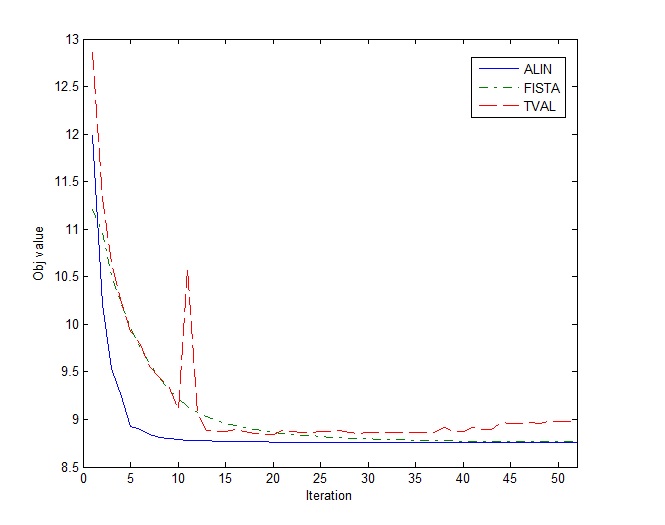
Although TVAL has superior performance in terms of running time, when compared to FISTA and ALIN, it produces an image of lower quality. With the same value of parameter , TVAL was not able to obtain the same objective function value as FISTA and ALIN. This makes the SNR of the TVAL-restored image lower and the error higher than those of ALIN and FISTA. ALIN and FISTA have similar performance in terms of image quality, but ALIN is more efficient than FISTA. In Figure 7, we plot the progression in terms of objective function values for all three methods. TVAL takes only 52 iterations to terminate. In this plot, ALIN and FISTA are set to terminate in 52 iterations.
In the second comparison, we pick random grayscale images with medium size, ranging from to pixels. The experiment is carried out in the same manner as the previous one. The results are reported in Table 4, and we observe the same pattern as in the previous comparison.
| Method | CPU time (secs) | SNR | MSE |
|---|---|---|---|
| FISTA | 65.41 | 12.14 | 5.98 |
| ALIN | 41.28 | 12.14 | 5.97 |
| TVAL | 7.18 | 8.30 | 14.36 |
5.5 Application to a narrative comprehension study for children
With high dimensional fused lasso penalty, the constrained optimization problem with identity design matrix is already difficult to solve, and a large body of literature has been devoted to solving this problem. When the design matrix is not full rank, the problem becomes much more difficult. In this section, we apply the three-dimensional fused lasso penalty to an regression problem where the design matrix contains many more columns than rows.
Specifically, we perform regularized regression between the measurement of children’s language ability (the response ) and voxel level brain activity during a narrative comprehension task (the design matrix ). Children develop a variety of skills and strategies for narrative comprehension during early childhood years (Karunanayaka et al., 2010). This is a complex brain function that involves various cognitive processes in multiple brain regions. We are not attempting to solve the challenging neurological problem of identifying all such brain regions for this cognitive task. Instead, the goal of this study is to demonstrate ALIN’s ability for solving constrained optimization problems of this type and magnitude.
The functional MRI data are collected from 313 children with ages 5 to 18 (Schmithorst et al., 2006). The experimental paradigm is a 30-second block design with alternating stimulus and control. Children are listening to a story read by adult female speaker in each stimulus period, and pure tones of 1-second duration in each resting period. The subjects are instructed to answer ten story-related multiple-choice questions upon the completion of the MRI scan (two questions per story). The fMRI data were preprocessed and transformed into the Talairach stereotaxic space by linear affine transformation. A uniform mask is applied to all the subjects so that they have measurements on the same set of voxels.
The response variable is the oral and written language scale (OWLS). The matrix records the activity level for all the 8000 voxels measured. The objective function is the following:
where
and , , and .

While the main purpose of this study is to demonstrate the capability of the ALIN algorithm for solving penalized regression problems with 3-d fused lasso, there are also some interesting neurological observations. One objective of this study is to identify the voxels that are significant for explaining the performance score . These voxels constitute active brain regions that are closely related to the OWLS. Figure 8 presents the results of fitted coefficients using combined lasso and fused lasso penalty. The highlighted regions shown in the maps are areas with more than 10 voxels (representing clusters of size 10 and above). The left plot in the figure is the optimal solution obtained using ten-fold cross validation. The optimal tuning parameters are 0.2 for both fused lasso and lasso penalties. Roughly speaking, five brain regions have been identified. The yellow area to the rightmost side of the brain is situated in the wernicke area, which is one of the two parts of the cerebral cortex linked to speech. It is involved in the understanding of written and spoken language. The only difference between the left and right plots is the value of the tuning parameter for the lasso penalty, which is 0.2 and 0.6 respectively. Clearly, the right plot shrinks more coefficients to zero, which results in a reduced number of significant regions, as compared to the left plot.

We further study this regularization problem using only lasso penalty and Tiknonov type penalty similar to (33). Figure 9 shows the fitted maps. The left plot is the case where only lasso penalty is applied. Comparing this with Figure 8, we see that the 3-d fused lasso penalty imposes smoothing constraints on the neighboring coefficients, thus allowing to identify larger areas significant for the response variable . The simple lasso penalty imposes shrinkage on the coefficients individually, resulting in rather disjoint significant voxels. Such scatterness is much less informative for neurologists than larger areas identified by the three-dimensional fused lasso penalty. Meanwhile, the Tiknonov type regularization generates too many significant regions as shown in the right plot. This is partially due to the over smoothing of the image as discussed in the previous section.
For comparison, we have considered a couple of methods designed to solve this particular problem. Genlasso is the path algorithm designed for the Generalized Lasso in the original paper. However, it was unable to handle an instance of this magnitude.
Another method is the Augmented Lagrangian and Alternating Direction method. The problem of interest
| (35) |
can be reformulated as
| (36) |
The Augmented Lagrangian is:
| (37) |
where is the penalty coefficient. This formulation can be solved by the Alternating Direction method. We implemented this method in Matlab. The update step for requires minimizing a quadratic function. The iterative method of choice to solve the sub-problems is the conjugate gradient method built in Matlab. The performance of this method strongly depends on the choice of the penalty parameter . As suggested in (Wahlberg et al., 2012), we choose to keep the algorithm stable for the implementation. It is known that the method has a nice decrease in the function values but slow tail convergence and an iteration of ADMM for this particular problem is rather expensive so we let it run for iterations and let ALIN run until it reached the same objective function value. The running times for different values of are reported in Table 5.
| Method | |||||
|---|---|---|---|---|---|
| CPU time (secs) | CPU time (secs) | CPU time (secs) | CPU time (secs) | CPU time (secs) | |
| ALIN | 20.68 | 12.19 | 18.58 | 23.45 | 129.81 |
| ADMM | 72.86 | 94.69 | 68.13 | 74.43 | 267.01 |
We also implemented FISTA for this particular problem. For each iteration of FISTA, the following optimization problem is solved:
| (38) |
where is Gaussian loss function and . The parameter is the Lipschitz constant of . This problem is similar to the f-subproblem of ALIN, so we utilize our own block-coordinate descent method to solve this problem. Since the Lipschitz constant cannot be computed efficiently, we use back-tracking to find the proper . Back-tracking is a popular method to find the right step size for FISTA iterations, however it can slow down the algorithm significantly. We observe that in each iteration, back-tracking will have to solve the sub-problem to times to find a good approximation to the Lipschitz constant of . Normally, this quantity is approximated by the maximum eigenvalue of . However, in the setting, it is not computationally efficient to estimate eigenvalues. When FISTA is applied to this data set with 3-d fused lasso penalty, it needs around iterations to reach the same objective function value as ADMM, and the running time is more or less an hour. This is also in line with what we observe from the implementation of FISTA for 1-d fused lasso penalty in the package SPAMS.
6 Conclusion
The alternating linearization method is a specialized nonsmooth optimization method for solving structured nonsmooth optimization problems. It combines the ideas of bundle methods and operator splitting methods, to define a descent algorithm in terms of the values of the function that is minimized. We have adapted the alternating linearization method to structured regularization problems by introducing the idea of diagonal quadratic approximation and developing specialized methods for solving subproblems. As a result, a new general method for a variety of regularization problems has been obtained, which has the following theoretical features:
- •
It deals with nonsmoothness directly, not via approximations,
- •
It is monotonic with respect to the values of the function that is minimized,
- •
Its convergence is guaranteed theoretically.
Our numerical experiments on a variety of structured regularization problems illustrate the applicability of the alternating linearization method and indicate its practically important virtues: speed, scalability, and accuracy. It clearly outperforms extant methods, and it can solve problems which were unsolvable otherwise.
Its efficacy and accuracy follow from the use of the diagonal quadratic approximation and from a special test, which chooses in an implicit way the best operator splitting step to be performed. The current approximate solution is updated only if it leads to a significant decrease of the value of the objective function.
Its scalability is due to the use of highly specialized algorithms for solving its two subproblems. The algorithms do not require any explicit matrix formation or inversion, but only matrix–vector multiplications, and can be efficiently implemented with sparse data structures.
References
- Bauschke and Combettes (2011) H. H. Bauschke and P. L. Combettes. Convex analysis and monotone operator theory in Hilbert spaces. CMS Books in Mathematics/Ouvrages de Mathématiques de la SMC. Springer, New York, 2011.
- Beck and Teboulle (2009) A. Beck and M. Teboulle. A fast iterative shrinkage-thresholding algorithm for linear inverse problems. SIAM Journal on Imaging Sciences, 2(1):183–202, 2009.
- Birgin and Martínez (2002) E. G. Birgin and J. M. Martínez. Large-scale active-set box-constrained optimization method with spectral projected gradients. Comput. Optim. Appl., 23(1):101–125, 2002.
- Bonnans et al. (2003) J.-F. Bonnans, J. C. Gilbert, C. Lemaréchal, and C. Sagastizábal. Numerical Optimization. Theoretical and Practical Aspects. Springer-Verlag, Berlin, 2003.
- Boyd et al. (2010) S. Boyd, N. Parikh, E. Chu, B. Peleato, and J. Eckstein. Distributed optimization and statistical learning via the alternating direction method of multipliers. Foundations and Trends in Machine Learning, 3(1):1–122, 2010.
- Chen et al. (2010) X. Chen, S. Kim, Q. Lin, J. Carbonell, and E. Xing. Graph-structured multi-task regression and an efficient optimization method for general fused lasso. technical report 1005.3579v1, arXiv, 2010.
- Chen et al. (2012) X. Chen, Q. Lin, S. Kim, J. Carbonell, and E. Xing. Smoothing proximal gradient method for general structured sparse regression. Ann. Appl. Stat., 6(2):719–752, 2012.
- Combettes (2009) P. L. Combettes. Iterative construction of the resolvent of a sum of maximal monotone operators. J. Convex Anal., 16(3-4):727–748, 2009.
- Combettes and J.-C. (2011) P. L. Combettes and Pesquet J.-C. Proximal splitting methods in signal processing. In Fixed-Point Algorithms for Inverse Problems in Science and Engineering, Springer Optimization and Its Applications, pages 185–212. Springer, 2011.
- Daubechies et al. (2004) I. Daubechies, M. Defrise, and C. De Mol. An iterative thresholding algorithm for linear inverse problems with a sparsity constraint. Comm. Pure Appl. Math, 57(11):1413–1457, 2004.
- Douglas and Rachford (1956) J. Douglas and H. H. Rachford. On the numerical solution of heat conduction problems in two and three space variables. Trans. Amer. Math. Soc., 82:421–439, 1956.
- Eckstein and Bertsekas (1992) J. Eckstein and D. P. Bertsekas. On the Douglas-Rachford splitting method and the proximal point algorithm for maximal monotone operators. Math. Programming, 55(3, Ser. A):293–318, 1992.
- Efron et al. (2004) B. Efron, T. Hastie, I. Johnstone, and R. Tibshirani. Least angle regression. Annals of Statistics, 32(2):407–451, 2004.
- Fadili and Peyré (2011) J.M. Fadili and G. Peyré. Total variation projection with first order schemes. IEEE Transactions on Image Processing, 20(3):657 –669, 2011.
- Friedlander and Martínez (1994) A. Friedlander and J. M. Martínez. On the maximization of a concave quadratic function with box constraints. SIAM J. Optim., 4(1):177–192, 1994.
- Friedman et al. (2007) J. Friedman, T. Hastie, H. Hoefling, and R. Tibshirani. Pathwise coordinate optimization. Annals of Applied Statistics, 1(2):302–332, 2007.
- Fu (1998) W. Fu. Penalized regressions: the bridge vs. the lasso. Journal of Computational and Graphical Statistics, 7(3):397–416, 1998.
- Goldfarb et al. (2013) D. Goldfarb, S. Ma, and K. Scheinberg. Fast alternating linearization methods for minimizing the sum of two convex functions. Mathematical Programming, (141):349–382, 2013.
- Goldstein and Osher (2009) T. Goldstein and S. Osher. The split Bregman method for -regularized problems. SIAM J. Imaging Sci., 2(2):323–343, 2009.
- Golub and Van Loan (1996) G. H. Golub and C. F. Van Loan. Matrix Computations. Johns Hopkins Studies in the Mathematical Sciences. Johns Hopkins University Press, Baltimore, MD, third edition, 1996.
- Grosenick et al. (2011) L. Grosenick, B. Klingenberg, B. Knutson, and J. Taylor. A family of interpretable multivariate models for regression and classification of whole-brain fmri data. 2011.
- Grosenick et al. (2013) L. Grosenick, B. Klingenberg, K. Katovich, B. Knutson, and J. Taylor. Interpretable whole-brain prediction analysis with graphnet. Neuroimage, 2013.
- He and Yuan (2011) B. He and X. Yuan. On the convergence rate of alternating direction method. Technical report, Optimization On-Line, 2011.
- Hiriart-Urruty and Lemaréchal (1993) J.-B. Hiriart-Urruty and C. Lemaréchal. Convex analysis and minimization algorithms. II, volume 306 of Grundlehren der Mathematischen Wissenschaften [Fundamental Principles of Mathematical Sciences]. Springer-Verlag, Berlin, 1993.
- Hoefling (2010) H. Hoefling. A path algorithm for the fused lasso signal approximator. Journal of Computational and Graphical Statistics, 19(4), 2010.
- Karunanayaka et al. (2010) P. Karunanayaka, V. J. Schmithorst, J. Vannest, J. P. Szaflarski, E. Plante, and S. K. Holland. A group independent component analysis of covert verb generation in children: A functional magnetic resonance imaging study. Neuroimage, 51:472–487, 2010.
- Kiwiel et al. (1999) K. Kiwiel, C. Rosa, and A. Ruszczyński. Proximal decomposition via alternating linearization. SIAM Journal on Optimization, 9:153–172, 1999.
- Kiwiel (1985) K. C. Kiwiel. Methods of descent for nondifferentiable optimization, volume 1133 of Lecture Notes in Mathematics. Springer-Verlag, Berlin, 1985.
- Li et al. (2013) C. Li, W. Yin, H. Jiang, and Y. Zhang. An efficient augmented lagrangian method with applications to total variation minimization. Computational Optimization and Applications, 56(3), 2013.
- Lions and Mercier (1979) P.-L. Lions and B. Mercier. Splitting algorithms for the sum of two nonlinear operators. SIAM J. Numer. Anal., 16(6):964–979, 1979.
- Liu et al. (2010) J. Liu, L. Yuan, and J. Ye. An efficient algorithm for a class of fused lasso problems. ACM SIGKDD Conference on Knowledge Discovery and Data Mining, 2010.
- Liu et al. (2011) J. Liu, L. Yuan, and J. Ye. SLEP: Sparse learning with efficient projections. technical report, Computer Science Center, Arizona State University, 2011.
- Michel et al. (2011) V. Michel, A. Gramfort, G. Varoquaux, E. Eger, and B. Thirion. Total variation regularization for fmri-based prediction of behavior. IEEE Transactions on Medical Imaging, 30(7):1328–1340, 2011.
- Nesterov (2007) Yu. Nesterov. Gradient methods for minimizing composite objective function. discussion paper 2007/76, ECORE, 2007.
- Peaceman and Rachford (1955) D. W. Peaceman and H. H. Rachford. The numerical solution of parabolic and elliptic differential equations. J. Soc. Indust. Appl. Math., 3:28–41, 1955.
- Qin and Goldfarb (2012) Z. Qin and D. Goldfarb. Structured sparsity via alternating direction methods. Journal of Machine Learning Research, pages 1435–1468, 2012.
- Ruszczyński (1995) A. Ruszczyński. On convergence of an augmented Lagrangian decomposition method for sparse convex optimization. Math. Oper. Res., 20(3):634–656, 1995.
- Ruszczyński (2006) A. Ruszczyński. Nonlinear optimization. Princeton University Press, Princeton, NJ, 2006.
- Schmithorst et al. (2006) V. Schmithorst, S. Holland, and E. Plante. Cognitive modules utilized for narrative comprehension in children: a functional magnetic resonance imaging study. Neuroimage, 29:254–266, 2006.
- Tibshirani (1996) R. Tibshirani. Regression shrinkage and selection via the lasso. Journal of The Royal Statistical Society Series B, 58(1):267–288, 1996.
- Tibshirani and Taylor (2011) R. Tibshirani and J. Taylor. The solution path of the generalized lasso. Annals of Statistics, 39(3), 2011.
- Tibshirani and Wang (2008) R. Tibshirani and P. Wang. Spatial smoothing and hot spot detection for cgh data using the fused lasso. Biostatistics, 9(1):18–29, 2008.
- Tibshirani et al. (2005) R. Tibshirani, M. Saunders, J. Zhu, and S. Rosset. Sparsity and smoothness via the fused lasso. Journal of The Royal Statistical Society Series B, 67:91–108, 2005.
- Tseng (2001) P. Tseng. Convergence of block coordinate descent method for nondifferentiable minimization. Journal of Optimization Theory and Applications, 109:474–494, 2001.
- Wahlberg et al. (2012) B. Wahlberg, S. Boyd, M. Annergren, and Y. Wang. An admm algorithm for a class of total variation regularized estimation problems. arXiv:1203.1828, 2012.
- Wang et al. (2008) Y. Wang, J. Yang, W. Yin, and Y. Zhang. A new alternating minimization algorithm for total variation image reconstruction. SIAM Journal on Imaging Sciences, 1(3):248–272, 2008.
- Wright et al. (2009) S. Wright, R. Nowak, and M. Figueiredo. Sparse reconstruction by separable approximation. IEEE Transactions on Signal Processing, 57(7), 2009.
- Ye and Xie (2011) G.-B. Ye and X. Xie. Split Bregman method for large scale fused Lasso. Comput. Statist. Data Anal., 55(4):1552–1569, 2011.
- Zhang et al. (2012) Z. Zhang, K. Lange, and C. Sabatti. Reconstructing dna copy number by joint segmentation of multiple sequences. BMC Bioinformatics, 13(205), 2012.