Topologies and Price of Stability of Complex Strategic Networks with Localized Payoffs : Analytical and Simulation Studies
Abstract
Several real-world networks exhibit a complex structure and are formed due to strategic interactions among rational and intelligent individuals. In this paper, we analyze a network formation game in a strategic setting where payoffs of individuals depend only on their immediate neighbourhood. We call these payoffs as localized payoffs. In this network formation game, the payoff of each individual captures (1) the gain from immediate neighbors, (2) the bridging benefits, and (3) the cost to form links. This implies that the payoff of each individual can be computed using only its single-hop neighbourhood information. Based on this simple and appealing model of network formation, our study explores the structure of networks that form, satisfying one or both of the properties, namely, pairwise stability and efficiency. We analytically prove the pairwise stability of several interesting network structures, notably, the complete bi-partite network, complete equi-k-partite network, complete network and cycle network, under various configurations of the model. We validate and further extend these results through extensive simulations. We then characterize topologies of efficient networks by drawing upon classical results from extremal graph theory and discover that the Turan graph (or the complete equi-bi-partite network) is the unique efficient network under many configurations of parameters. We next examine the tradeoffs between topologies of pairwise stable networks and efficient networks using the notion of price of stability, which is the ratio of the sum of payoffs of the players in an optimal pairwise stable network to that of an efficient network. Interestingly, we find that price of stability is equal to for almost all configurations of parameters in the proposed model; and for the rest of the configurations of the parameters, we obtain a lower bound of on the price of stability. This leads to another key insight of this paper: under mild conditions, efficient networks will form when strategic individuals choose to add or delete links based on only localized payoffs.
I Introduction
Several real world networks such as the Internet, social networks, organizational networks, biological networks, food webs, co-authorship networks, citation networks, and many more exhibit complex network structures. Complex networks, generally modeled as graphs in most of the mathematical literature, have been extensively studied in recent years and they are pervasive in today’s science and technology [1, 2, 3, 4]. Studying the properties of the complex network structures helps to understand the underlying phenomena and developing new insights into the system such as small-world phenomena, scale-free topology, and structural holes [5, 6, 4, 7, 8].
Complex networks have also been studied extensively in the social sciences [4, 9, 10, 11] (and the references therein). These studies reveal that complex social networks play an important role in spreading information [12, 13, 14, 15, 16, 17]. Individuals that participate in the process of information dissemination in such networks receive various kinds of social and economic incentives and at the same time they also incur costs in forming and maintaining the contacts (i.e. links) with other individuals in terms of time, money, and effort. For this reason, individuals do act strategically while selecting their neighbors. Thus, in several contexts, the behavior of the system is driven by the strategic actions of a large number of individuals, each motivated by self-interest and optimizing an individual objective function. Thus, it is important to study the dynamics of strategic interaction among the individuals in complex social networks in order to understand how such networks form and this is the primary motivation for this paper.
Many recent studies on network formation have used game theoretic approaches [18, 19, 20, 21, 22, 23, 24, 25, 26] based on the observation that individuals are strategic and are interested in maximizing their payoffs from the social interactions. These models capture the strategic interactions among individuals and the analysis of these models satisfactorily deduces the topologies of equilibrium networks. In this domain, networks that are enforced by a central authority are known as efficient networks. Understanding the compatibility between equilibrium networks and efficient networks has been the primary focus of research in network formation [27, 19, 20, 28, 29, 30, 31, 32].
The crux of most of the models for network formation in the literature [27, 33, 34, 35, 36, 30, 31] is the underlying strategic form game where the players, strategies, and utilities (also termed as payoffs) are defined as follows: (i) the individual agents in the complex network are the players, (ii) the strategy of each agent is a subset of other agents with which it wishes to form links, and (iii) the utility of each agent depends on the structure of the network.
Another key aspect of most of the existing work in the literature is that the process of network formation is modeled in a decentralized fashion where the individuals in the network take autonomous decisions regarding whether to form or delete links with other agents. However, most of these models require the agents to know the complete global structure (that is, information about all nodes as well as all the links between the nodes) of the network to compute their respective payoffs. In many practical scenarios, this will be a very demanding requirement making the utility computation a cumbersome and often intractable task. Moreover, empirical evidence [8, 37] has clearly shown that a significant fraction of the perceived social and economic benefits for the individuals is derived from their -hop or -hop neighborhood. Motivated by this, a few models of network formation have been investigated that use local information (such as information about -hop or -hop neighborhood). For instance, Kleinberg and co-authors [38] propose a network formation model where the utility function of each node is based on -hop neighborhood information. However, in several real-world examples, we observe that complete knowledge about -hop information may be infeasible and nodes may need to get a reasonably accurate estimate of their payoffs by using just their immediate neighborhood (or -hop) information. In fact, we can observe such constraints in several real-world examples like distributed sensor networks and real-life social networks. In distributed sensor networks, coalitions of sensors can work together to track targets of interest and each sensor knows only its immediate neighborhood. In real-life social networks, it may not be possible for an individual to know all the friends of his/her immediate friends. Note that individuals can know partial information about their -hop neighborhood (i.e. friends of friends); however, this partial information is inadequate to accurately compute the payoffs of the individuals. Hence, in such settings, it becomes important to study the network formation process using only single hop neighborhood information and this is the primary motivation behind our work in this paper.
In this paper, we explore a novel model of network formation process from an economic perspective in which individuals derive payoffs (consisting of benefits from immediate neighbors as well as structural holes and the costs to form links) using purely local neighbourhood information and we refer to this setting as network formation with localized payoffs. The primary contribution of our work is to come up with a game theoretic model in the above setting and study the topologies of the equilibrium networks and efficient networks that emerge in such a network formation process. We next examine the tradeoffs between topologies of equilibrium networks and efficient networks using the notion of price of stability [35]. Informally, price of stability is the ratio of the sum of payoffs of the players in an optimal (in terms of sum of payoffs of the players) pairwise stable network to that of an efficient network. Interestingly, we find that price of stability is for almost all configurations of the parameters in the proposed model; and for the rest of the configurations of the parameters in the proposed model, we obtain a lower bound of on price of stability. This indicates that, when some mild conditions are satisfied, efficient networks will form when strategic individuals choose to add or delete links based on localized payoffs.
We note that our model assumes that a link forms with the consent of both the individuals (refer to Section II), as social contacts usually emerge in this manner. This assumption is widely considered in several models of network formation in the literature [29, 33, 28, 39, 40, 41]. In such situations, an appropriate choice for the notion of equilibrium is pairwise stability [33]. Informally, we call a network pairwise stable if no agent can improve its utility by deleting any link and no two unconnected individuals can form a link to improve their respective payoffs. We call a network efficient if the sum of payoffs of the individuals is maximal. In this framework, our objective is to investigate the tradeoff between topologies of pairwise stable and efficient networks. In the rest of the paper, we use the terms graph and network interchangeably. We thus use the terms nodes and individuals interchangeably throughout the paper. As a game-theoretic approach is used, we sometimes use the terms players and individuals interchangeably throughout the paper.
I-A Relevant Work
The field of network formation has been extensively studied in diverse fields such as sociology, physics, computer science, economics, mathematics and biology [19, 20, 21, 22, 28, 29, 42, 43, 38, 44, 45, 46, 24, 23, 31, 33, 32, 47, 48, 39, 49, 50, 25, 26]. In this section, we have included a discussion of the models that are most relevant to our work.
The modeling of strategic formation in a general network setting was first studied in the seminal work of Jackson and Wolinsky [33]. They basically consider a value function and an allocation rule model where the value function defines a value to each network and the allocation rule distributes this value to the nodes in the network. They investigate whether efficient networks will form when self-interested individuals can choose to form links and/or break links. The authors define two stylized models. For these models, the authors observe that for high and low costs the efficient networks are pairwise stable, but not always for medium level costs. They also examine the tension between efficiency and stability and derive various conditions and allocation rules for which efficiency and pairwise stability are compatible. An important feature their model does not capture is that of the intermediary benefits that nodes gain by being intermediaries lying on the paths between non-neighbor nodes. In particular, they do not capture the benefits due to structural holes.
Hummon [28] carries out several interesting investigations to unravel more specific topologies using a specific model proposed by Jackson and Wolinsky [33]. Two different agent-based simulation approaches, the multi-thread model and the discrete event simulation model, are used in the analysis done by Hummon [28] to explore the dynamics of network evolution based on a model proposed in Jackson and Wolinsky [33]. Hummon identifies certain pairwise stable structures that are more specific than those anticipated by the formal analysis of Jackson and Wolinsky [33]. Doreian [29] explores the same issue in a systematic manner and establishes the conditions under which different pairwise structures are generated. Some gaps in the analysis of Doreian [29] are addressed by Xie and Cui [40, 41].
Jackson [39] reviews several models of network formation in the literature with an emphasis on the tradeoffs between efficiency with stability. This work also studies the relationship between pairwise stable and efficient networks in a variety of contexts and under three different definitions of efficiency. A later paper by Jackson [47] presents a family of allocation rules (for example, networkolus) that incorporate information about alternative network structures when allocating the network value to the individual nodes. The author provides a general method of defining allocation rules in network formation games.
Goyal and Vega-Redondo [43] propose a non-cooperative game model in which a node can benefit from serving as an intermediary between a pair of nodes and . In their model, a node could lie on an arbitrarily long path between and . The authors assume, however, that the benefits from farther nodes are not subject to decay. They also assume that the benefit of communication between any pair of nodes is always unit. This unit is distributed to the two communicating nodes and only to certain so called essential nodes [43] on the paths between the two communicating nodes. In this setting, the authors show that a star graph is the only non-empty robust equilibrium graph. The authors also study the implications of capacity constraints in the ability of individual nodes to form links to other nodes and show that a cycle network emerges.
Ramasuri and Narahari [51] propose a generic model of network formation that essentially builds on the model of Jackson-Wolinsky [33]. This model simultaneously captures four key determinants of network formation: (i) benefits from immediate neighbors through links, (ii) costs of maintaining the links, (iii) benefits from non-neighboring nodes and decay of these benefits with distance, and (iv) intermediary benefits that arise from multi-step paths. The authors [51] analyze the proposed model to determine the topologies of stable and efficient networks.
The aforementioned models of network formation have the limitation that each individual (or node) needs to know global information about the structure of the network in order to compute its utility. A few recent models [42, 52, 38] in the literature make an attempt to overcome the above limitation.
- •
Buskens and van de Rijt [42] propose a model that requires each individual agent to know just its immediate neighbors (or -hop neighborhood) to optimize its own utility. However, the model captures only the cost to nodes and ignores various benefits that nodes can derive from the network such as direct benefits from the neighbors and the bridging benefits.
- •
Arcaute, Johari, and Mannor [52] study the myopic dynamics in network formation games. A key aspect of the dynamics studied in this model is the local information and the authors show that these dynamics converge to efficient or near efficient outcomes. However, the model does not characterize the topologies of equilibrium and efficient networks. Moreover, the model works with Pareto efficiency whereas we work with a more natural notion of efficiency, namely maximizing the sum of payoffs of all the nodes.
- •
Kleinberg and co-authors [38] characterize the structure of stable networks with Nash equilibrium as the notion of stability. The authors propose a polynomial time algorithm for a node to determine its best response in a given graph as nodes can choose to link to any subset of other nodes. They also show that stable networks have a rich combinatorial structure. However, the model needs each individual agent to know its -hop neighborhood (the set of all individuals that are reachable within two hops) to compute and optimize its own utility. The model works with Nash equilibrium while our proposed model works with the more natural notion of pairwise stability as the notion of equilibrium. Also, our model considers only single hop neighbourhood which is more appropriate for certain kinds of social networks as already explained. Moreover, the model [38] does not study the tradeoff between the topologies of stable networks and the topologies of efficient networks.
I-B Our Contributions
To the best of our knowledge, our current study is the first one to comprehensively explore the tradeoff between pairwise stability and efficiency using the notion of price of stability in the context of strategic network formation with localized payoffs, while taking into account several key factors such as link costs, link benefits, and bridging benefits. The following are the specific contributions of our paper.
- •
Section II: An Elegant Model for Network Formation with Localized Payoffs: We propose a strategic form game to model the process of network formation with localized payoffs and we term the game as network formation (game) with localized payoffs (NFLP). The utility of each player in the proposed game takes into account not only the benefits () that arise from routing information to and from its neighbors but also the cost () to maintain a link to each of its neighbors.
- •
Section III: Analytical Characterization of Topologies of Pairwise Stable Networks: We first analytically characterize the topologies of the pairwise stable networks using the NFLP model. Some of the networks that we consider for analysis include the cycle, star, complete and null networks. In addition, we also derive pairwise stability conditions for certain classes of k-partite networks namely bipartite complete networks, complete equi-tri-partite networks and complete equi-k-partite networks. We note that our findings extend the possible topologies for pairwise stable networks compared to that of other models in the literature.
- •
Section IV: Simulation of Network Formation Process and Additional Insights: Next, we simulate strategic dynamics in NFLP to understand how pairwise stable networks evolve over time. Our simulation results validate our analytical deductions and also reveal additional interesting insights on the topologies of pairwise stable networks. In addition, we study the emergent pairwise stable topologies during the network formation process and study the evolution of pairwise stable network and its properties like the clustering co-efficient, convergence time, etc. over different configuration parameters.
- •
Section V: Analytical Characterization of Topologies of Efficient Networks: Next, we analytically characterize topologies of efficient networks by drawing upon classical results from extremal graph theory. Our work leads to sharp deductions about the efficient networks in NFLP. A striking discovery of our study here is that the equi-bi-partite graph (popularly known as the Turan graph) emerges as the unique efficient network under many regions of values of and .
- •
Section VI: Price of Stability Investigations: The quality of optimal (in terms of the sum of payoffs of the individuals in the network) pairwise stable networks is best understood through the notion of price of stability (PoS). PoS allows us to explore the middle ground between centrally enforced solution and completely unregulated anarchy [35]. In most real-world applications, the nodes are not completely unrestricted in their strategic behavior but rather agree upon a prescribed equilibrium solution. In such scenarios, the prescription can be chosen to be the best equilibrium thus making the price of stability an important issue to study. We study the PoS in NFLP to reveal tradeoffs between pairwise stable networks and efficient networks. Intriguingly, we find that PoS is for almost all configurations of and . For the remaining configurations of and , we obtain a lower bound of on PoS. This implies, under mild conditions on and , that the proposed NFLP model produces pairwise stable networks that are efficient.
II A Model for Network Formation with Localized Payoffs
We model network formation using a strategic form game [18]. We consider a network setup with players denoted by . A strategy of a player is any subset of players with which the player would like to establish links. We assume that the formation of a link requires the consent of both the players. Assume that is the set of strategies of player . Let be a profile of strategies of the players. Also let be the set of all such strategy profiles. Each strategy profile leads to an undirected graph and we represent it by . If there is no confusion, we just use . If players and form a link in a graph , then we represent the new graph by . We assume that players in the network communicate using shortest paths - this is a standard assumption used in the literature for ease of modeling. In the rest the paper, we use the terms players, nodes, and agents interchangeably.
Degree of Node: The degree of node represents the number of neighbors of node .
Costs: If nodes and are connected by a link, then we assume that the link incurs a cost to each node. That is, if the degree of node is , then node incurs a cost of .
Benefits from Immediate Neighbors: Assume that . If node is connected to a node by a direct link, then we assume that node gains a benefit of . That is, if the degree of node is , then node gains a benefit of from its immediate neighbors.
Bridging Benefits: Consider a node . Assume that nodes and are two neighbors of node such that and are not connected by a direct link. Suppose that nodes and communicate using the length path through node , then (i) we assume that a benefit of arises due to this communication, and (ii) we also assume that the benefit entirely goes to node . We refer to as the bridging benefit to node . The main motivation for this kind of bridging benefits is by sociological studies suggesting that in practice most of the bridging benefits arise from bridging the communication between pairs of non-neighbor nodes in the network [53].
In this framework, we define the utility of node such that it depends on the benefits from immediate neighbors, the costs to maintain links to these immediate neighbors, and the bridging benefits. More formally, for any , the utility of node in an undirected graph is defined as follows:
| (1) |
where is the number of links among the neighbors of node in . There are two terms in this utility function. The first term specifies the net benefit to node from its immediate neighbors. The second term specifies the sum of bridging benefits to node . Here is the fraction of pairs of neighbors of node that are non-neighbors and normalizes the level of bridging benefits that node gains in the network.

For example, the fraction of pairs of neighbors of node that are non-neighbors in both and in Figure 1 is . However the degree of node in is and the degree of node in is . The normalization term ensures that the bridging benefit for node is higher in than in . Note that the bridging benefit of our proposed model can also be altered by introducing an arbitrary increasing, real-valued function of (call it ). In this case, the utility model (Equation 1) becomes as follows:
For ease of analysis, we work with throughout this paper.
Note: Assume that node bridges the communication between and ; and a benefit of is generated. In the literature, there are three well known ways of distributing the benefit to nodes , , and : (i) only node gets entire , (ii) node gets , and (iii) nodes , , and get equal share of . In this paper, we work with scenario (i). A similar approach is utilized in [38] as well. We note that the analysis that we perform using scenario (i) can be easily extended to other two scenarios.
II-A The Network Formation Game
The above framework defines a strategic form game that models network formation with localized payoffs. We refer to this as network formation game with localized payoffs (NFLP). The following example illustrates NFLP.
Example 1
Assume that is the set of players. If , , , , , , then the resultant graph is the star graph as shown in Figure 1.(i). Note that an edge forms with the consent of both the nodes.
Following the NFLP model, the payoffs of the players in the star graph are as follows: and .
If , , , , , , then the resultant graph is the wheel graph as shown in Figure 1.(ii). Following the NFLP model, the payoffs of the players in the wheel graph are as follows: and .
On similar lines, if , , , , , , then the resultant graph is the cycle graph as shown in Figure 1.(iii). Following the NFLP model, the payoffs of the players in the cycle graph are as follows: .
III Analytical Deductions on Topologies of Pairwise Stable Networks
In this section, we first recall the notion of pairwise stability. Then, we characterize the topologies of pairwise stable networks. To begin with, we note that the notion of pairwise stability is defined by Jackson and Wolinsky [33]. Formally, we call an undirected graph pairwise stable [33] if (i) and , (ii) , if then .
We now focus on characterizing the topologies of the pairwise stable networks that may emerge following the framework in NFLP. Characterizing pairwise stable networks under various network formation models has been addressed in the literature [19], [20], [42], [43], [38], [36], [30], [31], [33], [29], [49], [50]. In our approach, we consider the topologies of certain standard networks (such as complete network, cycle network, star network, multi-partite networks) and then study whether such topologies are pairwise stable following the framework of NFLP. We now present few results to establish certain standard networks are pairwise stable in the framework of NFLP.
Proposition 1
If and , then the complete bipartite network is pairwise stable.
Proof:
Consider a complete bipartite network, , with and
nodes respectively in the two partitions. The utility of node
in a partition with nodes is
. This proposition can be
proved in two steps.
Step 1: Let us now add the edge to and call the
resultant graph . It can be readily checked that
.
Since we are given that , we get that
. That
is, no pair of non-neighbor nodes is better off by forming a
link in .
Step 2: Assume that node severs an edge in and call
the resultant graph . It can be shown that
. Since we
are given that , it is immediately seen
that . Node is not better off by
severing a link in .
Note that we can apply similar analysis with respect to each node in the other partition. Hence the complete bipartite network is pairwise stable. ∎
Proposition 2
(a) The complete network is pairwise stable if (b) The cycle network is pairwise stable if , (c) The null (empty) network is pairwise stable if .
The result can be proved easily by using arguments similar to that in Proposition 1.
Proposition 3
For , the complete -partite network is pairwise stable if (i) , and (ii) where is the number of nodes in partition in -partite network and is any positive integer.
Proof:
We start with a -partite graph, , satisfying condition (ii) given in the statement of this proposition. Consider a node in the partition of where . We construct the proof in two steps.
Step 1 (edge addition): We can see that, in , the only link that can be added from node is to a node in the partition. Let be the network obtained after a new link is added to . For pairwise stability, we need . This implies
where is the number of links among the neighbours of node in and is the number of links among the neighbours of node in . Note that since nodes and belong to the same partition in . Now we get that . Simplifying, we get
| (2) |
Since the term lies in the interval and the fact that (given in the statement of this proposition), we get that expression (2) is non-positive. This implies that no pair of nodes can form a link to improve their respective payoffs.
Step 2 (edge deletion): In , consider that node deletes a link to a node in the partition where and . Let be the network obtained after the link has been deleted from . For pairwise stability, we need . This implies
where denotes the number of links among the neighbours of node in . We can see that . Simplifying,
| (3) |
Claim: .
Proof of the Claim: We know that . Now, we derive an expression for .
| (4) |
Now, we show that . The proof is by contradiction. Suppose .
| (5) |
From condition (2) in Proposition 3, we have and . Also, using Equation (4) in Equation (5) and simplifying, we have
| (6) | ||||
Let . As we know that the function is a decreasing function of (as derivative of with respect to is ), we can write
So, clearly we can conclude that for (i.e., and ) and for .
Now we will examine what happens when and . Substituting in Equation (6) and simplifying, we get which is absurd. Substituting in Equation (6) and simplifying, we get which violates the hypothesis that . Hence, by the above arguments, . This completes the proof of the claim.
Note that we are given that . Thus, from Equation (3),
Thus, node does not have any incentive to add an edge to or delete an edge from when the conditions given in the statement of the proposition are satisfied. As node is chosen arbitrarily from , we have that is pairwise stable. ∎
Using a similar approach, we can prove the stability results for other standard networks. We summarize these results in Table I11 1 Note that the legends in the figure correspond to the numbering specified in Table I and the graphical illustration of these results is depicted in Figure 2.
|
Parameter
Additional
P.S.11
1
Any correspondence can be addressed to rohithdv@gmail.com
Region
Conditions
networks
Complete
Complete
C.B.P 44footnotemark:
4
C.E.T.P 66footnotemark:
6
Complete
C.B.P
Complete, Null,
(2)
C.B.P,
C.E.K.P55footnotemark:
5
Null
C.B.P
Null
(3)
Cycle
Null
C.E.T.P
Null
C.B.P
11footnotemark:
1
P.S: Pairwise Stable
44footnotemark:
4
C.B.P: Complete BiPartite55footnotemark:
5
C.E.K.P: Complete Equi -Partite66footnotemark:
6
C.E.T.P: Complete Equi Tri-Partite
Table I: Characterization of pairwise stable
network topologies in the proposed utility model |
![[Uncaptioned image]](1201.0067v1/GraphicalIllustration_latest.png) Figure 2: Graphical Illustration
Figure 2: Graphical Illustration
|
IV Simulation: Validation and Additional Insights on Topologies
In this section, we investigate various aspects of the network formation game through extensive simulations. The main purpose of this exercise is to get a better understanding of the network formation process as theoretical analysis has limited scope in enabling the understanding of the cumulative effects of many of the parameters like the initial network density, cost-benefit values, scheduling order of the nodes, etc that influence the network formation process.
In the network formation process, starting from some initial configuration of a network, the resultant topology of pairwise stable network may not be any of the standard networks considered in the previous section. In other words, these simulation results reveal that there could exist certain other topologies that satisfy pairwise stability apart from these standard networks.
Starting with some initial network (the null network, for example), the network structure changes with time as various nodes in the network add or remove links to their neighbors, so as to maximize their own individual utility from the network. It would be interesting to determine if, in the long run, the network reaches a stable state (an equilibrium or a near-equilibrium state). If the network does reach a stable state, it would be interesting to know the structure (i.e. shape) of the stable network and if this stable network is unique. One way of approaching this is to start with the initial network and model the dynamics of the system as a function of time (or an analogous parameter) and analytically study the asymptotic network structure in the limit as time tends to infinity. However, the dynamics of the system can become very complex even in a moderately sized network, making such an approach infeasible. Further, such results would only be valid for those particular initial networks.
Another approach is to analyze the stability of some of the standard networks (complete network, cycle network, star network etc.) under our utility model (as presented in Table I). It would then mean that if the network reaches any of these standard stable networks, it is guaranteed to not deviate from this network. However, one problem with this approach is that starting from some initial network, we may not reach any of these standard networks. That is, some non-standard networks could be stable and the dynamic network could emerge into one of these non-standard networks.
IV-A Simulation Setup
We built a custom simulator using the C++ programming language in order to model the network formation process under our proposed network model. To implement the standard graph routines, we used the BOOST C++ libraries [54] which has efficient implementations of fundamental graph data structures and routines. We start with a random initial network consisting of nodes. The number of edges between these nodes is determined by the parameter . For example, if , we start with an empty network; if , we start with a network that contains of the possible edges. These edges are chosen uniformly at random. As noted in Section II, a node obtains a benefit of and incurs a cost ( ) for maintaining a direct relationship (represented by an edge) with another node. In addition, each node reaps additional indirect benefit because of its potential to bridge its unconnected neighbors (determined by sparsity of relationships among his neighbors).
IV-B The Simulation Process
We run the simulations for each combination of possible values of and as shown in Table II given below. A single simulation run refers to a simulation with a particular value of of and . Further, each simulation run is repeated multiple times as per the Num-Repetitions parameter. We now describe the details of a single simulation run below.
In a particular simulation run, each node is given an opportunity to act, based on a random schedule. Each node, when scheduled, considers three actions - namely, add an edge to a node that it is not directly connected to, delete an existing edge to a node, or do nothing. Each node chooses the action that maximizes its individual payoff (which is based on the parameters and ), breaking ties randomly. Node , when adding an edge to node , may be allowed to do so only if it is beneficial to both or if node is at least not worse off (mutual add (MA)). Similarly, node , when deleting an existing edge to node , may be allowed to do so unilaterally (unilateral delete). We study pairwise stable network evolution under these conditions.
Table II lists the various simulation parameters. At some stage in the simulation, the network could evolve into a stable state where no node has any incentive to modify the network. One iteration in which no node modifies the network is an idle iteration, and the parameter Num-Idle-Terminate indicates the number of idle iterations before we conclude that the network has reached a stable state. This is the case of normal termination of a simulation run. However, there may be cases where the network does not emerge into a stable state and cycles through previously visited states even after many iterations (the case of dynamic-equilibrium as noted in Hummon [28]). The parameter Max-Iterations indicates the number of iterations before we forcibly terminate the simulation run. However, we have observed that all the simulation runs achieved convergence much before the maximum iterations allowed indicating that the formation of dynamic equilibrium is not possible in our utility model. However, we leave the formal proof of this observation as a future work. The parameter Num-Repetitions indicates the number of times each simulation run was repeated. The simulations were averaged out over different initial conditions and random schedules.
| Parameters Values N 3, 4, 5, 10, 20 Cost (c) 0.05 to 1, in steps of 0.05 Benefit () 0.05 to 1, in steps of 0.05 Density () 0, 0.35, 0.7 Experiment Mutual-Add, Unilateral-Delete Num-Iterations 1000 Num-Repetitions 100 Num-Idle-Terminate 30 Table II: Simulation parameters and Values |
![[Uncaptioned image]](1201.0067v1/classify.png) Figure 3: A stylized 5-node network
Figure 3: A stylized 5-node network
|
IV-C Metrics Recorded
At the end of Num-Repetitions number of repetitions, a number of metrics were recorded. The following lists some of the important metrics recorded.
- 1.
The network structure (shape) for each repetition
- 2.
The frequency with which each of the network structures in Section IV-D resulted (across all repetitions)
- 3.
The mean utility of the final network (across all repetitions)
- 4.
The mean time to reach the final network (across all repetitions)
- 5.
The mean number of acts to reach the final network (across all repetitions)
Before we present the results, we briefly describe the classification criteria used to identify pairwise stable networks.
IV-D Classification of Pairwise Stable Network Structures
Once the network reaches a stable state, we classify the network structure as one of the network structures shown in Table III. As in Hummon [28], we use the sorted (descending order) degree vector to characterize the structure of the stable network. For example, the Null network has a sorted degree vector of (0, 0, …, 0), the Star network (n-1, 1, 1, …, 1) and the Complete network (n-1, n-1, …, n-1). We refer to a network structure a shared network if it is a regular network (i.e., all nodes have same degree) of some uniform degree. For example, a cycle is a -regular graph and hence is a shared network.
Also as in Hummon [28], we use total mean squared deviation (MSD) to classify the resultant stable network as Near-“standard network” (for example, Near-complete network). Further, if the mean squared deviation is above a certain threshold () then we know its not close to any of the above topologies, we then color the graph using a greedy coloring algorithm [54] and then classify it either as a general k-partite graph (where equals the number of colors required to color the graph) or any of the other network structures shown in Table III. In our simulations, we use the maximum deviation () for calculating the , i.e., .
Note that whenever we classify a network as any type of K-Partite network, we implicitly mean that . The case of is the same as bipartite network and is handled as a separately as shown in Table III. Turan network refers to a complete bipartite network with the sizes of the two partitions to be as equal as possible. If is even, then the Turan network has equal sized partitions whereas if is odd, the size of one partition is one less than the other partition.
For classification of a sorted degree network as a near-shared network, we first need to calculate the order of the regular network with which this degree vector needs to be compared. As in Hummon [28], to compute the total mean squared deviation for the shared structure, the ideal order is defined by average number of ties in the in-out degree vector, rounded to the nearest whole tie. In this example, if the degree vector is (3,2,1,1,1), the average is 1.6, and the ideal type shared structure is (2,2,2,2,2). However, note that a cycle network is necessarily a shared network but a shared network need not always be a cycle network.
| NULL | STAR | SHARED | COMPLETE |
|---|---|---|---|
| NEAR-NULL | NEAR-STAR | NEAR-SHARED | NEAR-COMPLETE |
| BI-PARTITITE-COMPLETE | TURAN | EQUI-K-PARTITE-COMPLETE | EQUI-K-PARTITE |
| K-PARTITE-COMPLETE | K-PARTITE |
The following example clarifies this procedure: Consider the -node network as shown in Figure 3. Suppose that we would like to classify this network as one of the following standard networks : Null, Star, Shared, Complete, Near-Null, Near-Star, Near-Shared or Near-Complete. This is done as follows. Note that the given network does not classify as any of the first four networks in the list given above. Hence, we try to classify the given network as one of the remaining four networks (i.e., the ‘near’ type networks).
We know that the sorted degree vector is for the given network. The ideal order for the shared network comparison is calculated by taking the average degree (which is ) and rounding to the nearest integer (which gives ). This means we have to compare the network to a -regular network. The total MSD from the shared network is thus . The total MSD of this network from Star network is . Similarly, the total MSD from Null network is , and the total MSD from the Complete Network is . The value being the least among these and less than of maximum deviation , we classify the above network structure as Near-Shared.
IV-E Multiple Classification of Pairwise Stable Structures
We note that the classification of pairwise stable network structures according to Table III is not mutually exclusive. There can exist networks which can be classified as more than one of the types described in Table III. We illustrate a couple of interesting network structures that we encountered during our simulations here. Figure 4(a) refers to a pairwise stable network that emerged when we ran the simulation with random_seed . We observed that this network is both a Near-Shared network as well as a Tri-partite complete network whose parititions are . In such cases, we classify the network structure as a K-Partite Complete network.

|

|
| (a) | (b) |
Another example is shown in Figure 4(b) which is obtained when running simulations with random_seed . We observe that this graph can be classified as a regular (or Shared) network with degree=. However, it turns out that this graph is also an equi-partitioned bipartite network with partitions . In such cases, we classify the graph as equi-bipartite network (or the Turan network).
IV-F Interpretation of Pairwise Stability
In a pairwise stable network, if a node adds a link to another node and gains strictly from it, the other node should lose strictly. Hence, the addition of the link becomes infeasible in this case. However, nodes in a pairwise stable network can still add links if adding these links does not change the payoffs of either of the nodes. In this case, the nodes are indifferent about adding the link. In the case of deletion, a node will delete a link from the current network unilaterally if it strictly benefits from doing so. We use this interpretation of pairwise stability during the course of our simulations.
IV-G Model Validation
We now proceed to understand some of the results of our simulations. First, in this section, we focus on the validation of our theoretical results on pairwise stability as shown in Figure 5. We are interested in knowing the following aspects in the simulations.
- •
Do the pairwise stable networks identified in Table I actually emerge in the simulation process?
- •
If so, under what values of and do they emerge?
- •
Do the conditions match with the theoretical results?

|

|

|
|
| (a) | (b) | (c) | (d) |

|

|

|

|
| (e) | (f) | (g) | (h) |

|

|

|

|
| (i) | (j) | (k) | (l) |

|

|

|

|
| (m) | (n) | (o) | (p) |

|

|
||
| (q) | (r) |
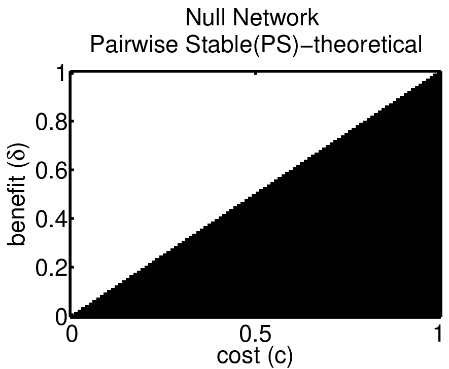
We conducted our simulations for all combinations of and as explained before. Figure 5(a)-Figure 5(r) validate the analytical results derived in Table I . The vertical axis of each plot in Figure 5 is the benefit value (), ranging from to , and the horizontal axis represents the cost parameter (), ranging from to . In general, given a particular value of and , there may be multiple network structures that may be pairwise stable. The type of network structure emerging in the network formation process depends on a number of factors like the initial network, the scheduling order of the nodes along with the parameters of and . Hence, we run each simulation run Num-Repetitions times each time starting with random schedules and starting with different initial networks with the hope of getting all possible pairwise stable networks. In particular, we start with three different initial networks with densities respectively as shown in Table II.
We plot the pairwise stable regions for different networks namely bipartite complete network, null network, complete network, etc and compare with the theoretical predictions. Figure 5(a)-(d) show theoretical results and Figure 5(e)-(r) show the results from the simulations.
Figure 5(e) shows the regions where the Bipartite Complete (BPC) network emerged as one of the pairwise stable network when the simulation run was started with number of nodes () and initial network with density(). Clearly, we can see that BPC does not emerge as pairwise stable in the regions where as the null network (which coincides with the initial network) is also pairwise stable and the nodes prefer not to add any links to the initial network. However, Figure 5(f) and Figure 5(g) show that if the starting network is already having some existing links then nodes try to form BPC network even in the regions where . This shows the importance of the initial network in the network formation process. Figure 5(h) is obtained by merging all the regions of Figure 5(e)-(g) and this closely corresponds to the theoretical predictions of BPC stability shown in Figure 5(a). Figure 5(i)-(l) similarly show results for . In this case, however, we observe that Figure 5(l) is not as close to Figure 5(a) which is due to the fact that there may be many more pairwise stable topologies that may emerge as the number of nodes increase which illustrates a fundamental difficulty in characterizing all pairwise stable networks for every possible value of number of nodes ().
Another observation is that the complete network is theoretically proven to be the unique pairwise stable network in the region shown in Figure 5(c). We can clearly see the simulation results in Figure 5(h) and Figure 5(l) that this region is clearly excluded from the BPC stable region as starting with any initial network, only the complete graph emerges as unique the pairwise stable network in the region specified by Figure 5(c).
We similarly show the stability regions for complete and null networks in Figure 5(m) and Figure 5(o) respectively which corresponds to the theoretical predictions of Figure 5(b) and Figure 5(d) respectively. As explained earlier, Figure 5(n) again illustrates the importance of initial network in making the null network as the pairwise stable network.
As shown in Proposition 3, the equi-kpartite network is stable when and Figure 5(p) shows that indeed in this region, the equi-kpartite network does emerge as the pairwise stable network when . Proposition 3 was only a sufficient condition, we observe from the figure that there are other regions of and (which we have not analytically characterized) at which equi-kpartite network emerges as the pairwise stable network.
As explained earlier, our characterization of pairwise stable network structures as shown in Table I is not exhaustive and hence, we used simulations to depict the region of stability for important types of network structures namely the near-shared network and k-partite complete network. We show the results in Figure 5(q) and Figure 5(r).
IV-H Emergent Network Topologies During Simulations

|

|

|

|

|

|
Figure 6 shows the simulation results for -node and -node networks. The exact parameter configurations and the initial network densities are marked in Figure 6. The vertical axis of each plot in Figure 6 is the benefit value (), ranging from to , and the horizontal axis represents the cost parameter (), ranging from to . As noted earlier, for a pair, we repeat the simulation for Num-Repetitions. Each repetition for the simulation results in a network that can be classified as one of the structures mentioned in the theoretical analysis. We plot the most frequent (modal ) network structure as determined by the frequency with which each of the network structures resulted in Num-Repetitions simulation runs. The experiment was repeated starting with different network densities, . We list some of the abbreviations used in the legends of the plots in Table 6.
| TUR_GRA | Turan Graph | BIPARCOMP | BiPartite Complete |
|---|---|---|---|
| NRSHARED | Near-Shared | KPARCOMP | KPartite Complete |
In each of the plots in Figure 6, we observe that the complete graph is the resultant pairwise stable network (when , ) which concurs with the theoretical deductions that the complete graph is the unique pairwise stable network in this region (Table I and Figure 5(c)).
We can also infer from Figure 5(a), Figure 5(b) and Figure 5(d) that there is an overlap in the stability regions among complete and complete bipartite and also between null and complete bipartite networks. However, as observed through simulations (Figure 6), we see that the complete bipartite network emerges as the modal pairwise stable network in its regions of overlap with the aforementioned networks. This can be attributed to the fact there are a large number of possible bipartite graphs whereas there is only one null network and one complete network. Hence, the likelihood of the null and complete emerging in a region where the bipartite network is also pairwise stable, is small.
We also observe from some of the plots in Figure 6 that Near-Shared and K-Partite Complete networks emerge as pairwise stable networks under some regions of the parameters. As explained in earlier sections, this can be attributed to the fact that our analytical results (as shown in Table I) is not exhaustive and there exist some new topologies ( which we characterize as Near-Shared or K-Partite Complete networks) which are also pairwise stable.
IV-I Network Evolution
Having studied the macroscopic behaviour of our simulations, we investigate the network formation process from a microscopic viewpoint. We examine various snapshots during the network formation process of a single simulation run which is repeated just once for a fixed parameter of and . We consider as our parameter configuration. We can observe from the our proposed utility model (Equation 1) that for this configuration the benefits from direct links is and so, nodes try to maximize the benefits due to bridging behavior. The nodes form/delete links such that they emerge as a bridge in connecting their unconnected neighbors. Hence, we would expect the final pairwise stable network to be consisting of nodes who are filling the positions of structural holes in the network. In other words, the emergent pairwise stable graph should be a triangle-free as nodes form links with nodes who are themselves are not connected with each other.
We depict the snapshots of network formation process in Figure 7. We can see that initially the nodes are forming links in such a way that triangles are not present but eventually triangles eventually do form due to the cumulative action of other nodes in the network. When triangles emerge in the neighbourhood of a node, it leads to deletion of links from that node (as the node will benefit strictly from deletion) and the final emergent network (Figure 7(l)) is a bipartite complete network (which is triangle-free) with alternate nodes in the ring layout depiction in Figure 7(l) belonging to the same partition.

|

|

|
| (a) | (b) | (c) |

|

|

|
| (d) | (e) | (f) |

|

|

|
| (g) | (h) | (i) |

|

|

|
| (j) | (k) | (l) |
In complex network literature, the number of triangles in the network is a important parameter which was first studied by Watts and Strogatz [5] by definition the notion of clustering, sometimes also known as network transitivity. Clustering refers to the increased propensity of pairs of people to be acquainted with one another if they have another acquaintance in common. Watts and Strogatz [5] define a clustering coefficient (denoted by ) that measures the degree of clustering in a undirected unweighted graph.
The factor three accounts for the fact that each triangle can be seen as consisting of three different connected triples, one with each of the vertices as central vertex, and assures that . A triangle is a set of three vertices with edges between each pair of vertices; a connected triple is a set of three vertices where each vertex can be reached from each other (directly or indirectly), i.e. two vertices must be adjacent to another vertex (the central vertex).
It can be observed from the utility model proposed in equation (1) in Section II that component in the utility model corresponds to the clustering coefficient of node . Thus, in our utility model, nodes benefit from having lesser clustering coefficient as this will lead to the formation of structural holes, which in turn leads to increase in the payoff for the node. We elaborate more on this when we discuss efficient network topologies in Section V.

|

|
| (a) | (b) |
We now study how the clustering coefficient changes as the network evolves through the different phases shown in Figure 7. We plot this result in Figure 8(a). We see that upto time epoch clustering coefficient is . Later there is a increase in the value which is followed by the reduction in the clustering coefficient back to (at time epoch ) when the pairwise stable network emerges. As explained before, this is indeed the expected behaviour during the network formation process for the parameters .
We also study the average clustering co-efficient in all the pairwise stable networks that emerge for different values of and . We take the average over running Num-repetitions number of times. The result is shown in the 3d plot in Figure 8 (b). We can see that the clustering coefficient assumes value of in the regions where the complete network is stable and when the null network is stable. In other regions, the clustering coefficient value is between and which indicates a tradeoff between the benefits from direct links and the benefits from bridging benefits to the nodes in the network.

|

|

|
| (a) | (b) | (c) |
IV-J Average Number of Actions before Convergence
In this section, we will study the effect the initial network density has on the effort needed by the nodes to achieve convergence to a pairwise stable network. A single addition of an edge or a single deletion of an edge by a node is considered to be a single ‘act’ by that player. We now study the mean number of acts performed by the players to converge to a pairwise stable network starting from various initial random networks. We can see from Figure 9(a) that the number of changes to the network is more when the region and this is because the initial network is a null network and the players need to perform a lot more additions/deletions to the network before reaching the final stable network which is the complete network. When , the players need not perform any change to the network as the initial null network is already pairwise stable. In fact, we can observe from the Figure 9 that the number of acts needed to reach the complete network is maximum (about ) when starting with null network than when compared to other scenarios of and (mean acts is about ).
We observe a reversal of the work needed to reach null network in Figure 9(c) where more number of changes is needed to reach null network than reaching the complete network. This can be attributed to the fact that the initial network is already a dense network to start with and it takes relatively less effort to reach the complete network than the null network under appropriate configurations of and .
Initial network density of corresponds to a medium-dense network (Figure 9(b)) and hence there is a non-zero effort to reach any of the pairwise stable network under any parameter configuration. However, as in Figure 9(a), it takes more effort for players to reach the complete network than the null network.
V Analytical Characterization of Topologies of Efficient Networks
In this section, we study the structure of efficient networks, i.e., networks that maximize the overall utility, under various conditions of and . First, we begin by introducing a few useful classical results in extremal graph theory and we use these results later in our analysis.
V-A Triangles in a Graph
If three nodes , , and in are such that and , and , and are connected by edges, then we say that nodes form a triangle in . The number of triangles in a simple graph plays a crucial role in the computation of payoffs to the nodes and we state here some classical results. We know from Turan’s theorem [55], that it is possible to have a triangle free graph if the following holds:
| (7) |
Here denotes the number of edges and the number of vertices of the graph. Moreover, from [56], we know that the number of triangles, , can be lower bounded, if the number of edges exceed the above value , by
| (8) |
In what follows, we refer to the graph having maximum number of edges with no triangles as the Turan Graph and we represent it by . It is easy to verify that such a graph is a complete bipartite graph, and the the number of vertices in each partition differs at most by .
V-B Finding the Efficient Graph
Definition 1 (Efficient Graph)
The utility ( of a given network is defined as the sum of payoffs of all the nodes in that network. That is,
| (9) |
A graph that maximizes the above expression (i.e. sum of payoffs of nodes) is called an efficient graph.
We now present a series of results on the topologies of efficient networks using the proposed framework. These results are based on different ranges for the values of and .
Proposition 4
When and , the null graph is the unique efficient graph.
Proof:
For any node , implies that the utility of that node is negative thus reducing the overall network utility. This follows from being negative. ∎
Proposition 5
When , the Turan graph is the unique efficient graph.
Proof:
We will analyze the efficiency of an arbitrary graph (denoted by ) as follows.
| (10) |
where, is the number of triangles in the graph . The last step of the above simplification is due to the fact that the number of links among the neighbours of a node is the number of triangles in the graph in which node is one of the vertices of the triangle. The factor in the last step is due to the fact that every triangle contributes to the of nodes. We know that, for an efficient graph, Equation (10) should be maximized and that happens when the number of triangles in a graph is minimized while simultaneously maximizing the number of edges in the graph.
The Turan graph (refer Equation (7)) is a graph with maximum edges that has no triangles. So an efficient graph must have an efficiency greater than or equal to that of a Turan graph. Thus, it is clear that there is no need to consider graphs with edges lesser than that of a Turan graph. Let us consider the case when a graph (denoted by ) has more edges than the Turan graph. Let have edges where . From Equation (10), we know that
| (11) |
where is the number of triangles in . From Equation (8), we have
| (12) |
Since , the efficiency of the Turan graph is:
| (13) |
The change in efficiency () between the two graphs is
| (14) |
which is clearly negative for any . This implies that the Turan graph is the unique efficient graph. ∎
Proposition 6
When and , the Turan graph is the unique efficient graph.
Proof:
We prove this by contradiction. Assume that is any graph other than the Turan graph and is efficient. We show below that cannot have lesser number of edges than ,
And observe, if has same number of edges as and is different from it, it can contain triangles and will have an utility less than that of , as the benefit from bridging would go down and the benefit from direct links would remain unchanged.
Thus contains more edges than . Observe, that the benefit from direct links is negative , and has an higher utility compared to that of . It has to be that the bridging benefits in has to be greater than that of the Turan graph, as the utility due to direct links term has become more negative compared to its value in
This implies that this graph would give a higher utility for the case, as the first term is there. This contradicts Theorem 5 and so our assumption must be wrong. Hence the Turan graph is efficient. ∎
| Parameter Range | Efficient Topologies |
|---|---|
| and | Null network |
| and | Turan network |
| Turan network | |
| and | Turan network |
| and | Complete network |
Proposition 7
When and , the Turan graph is the unique efficient graph.
Proof:
Let be the efficient graph. Using a similar analysis that lead to Equation (12), we can see that
| (15) |
For the Turan graph, it can also be seen by simple analysis that
| (16) |
Thus, when , the Turan graph is the unique efficient graph. ∎
Proposition 8
When and , the complete graph is the efficient graph.
Proof:
It can be shown that starting with an arbitrary graph (which is not a complete graph), adding an edge between two nodes and (with smallest degree) increases the cumulative utility of these two nodes by at least . At the same time, there is a decrease in utility of a common neighbour of nodes and , say node , as there is a decrease in the bridging benefits of node . It can be shown that the cumulative decrease in utility of all such common neighbours formed is which is less than equal to . Repeating the above process, we get the complete network. ∎
Conjecture 1
When and , the Turan graph is the efficient graph.
Conjecture 2
When and :
(i) if , then the complete graph is the efficient graph.
(ii) if , then the Turan graph is the efficient graph.
We summarize the above results on efficiency in Table V.
VI Price of Stability (PoS) of the Proposed Model
Recall that PoS [35] is the ratio of the sum of payoffs of the players in a best pairwise stable network to that of an efficient network. In NFLP, a best pairwise stable network means a pairwise stable network with a maximum value of the sum of payoffs of the players. By invoking the results derived in the previous sections, we now present our results on PoS for the proposed model.
Theorem 1
The price of stability (PoS) is in each of the following
scenarios:
(i) and ,
(ii) , and ,
(iii),
(iv) and .
Note: Since the null network is the only efficient network when and , PoS is not defined in this region.
In view of Conjecture 1, the following result presents bounds on PoS.
Proposition 9
When and , PoS .
Proof:
We know that, under the conditions and , the pairwise stable graph with the highest utility is the Turan graph (as seen from Table I). Let Conjecture 1 be false. In this scenario, let us denote the efficient graph by . We will now evaluate an upper bound on the maximum efficiency of . has to have more direct links than the Turan graph (as ) to be a candidate for efficient graph. Let have edges where .
Since can be at most ,
By Equation (8), we have
Since , we have
The Turan graph is pairwise stable under these conditions (refer Table I). Hence we get the following:
This implies that . ∎Remark: In view of Conjecture 2, it can be noted that a similar bound can be obtained in the region and . The details are not provided here due to space constraints.
VII Conclusions and Future Work
In this paper, we proposed a network formation game with localized payoffs (NFLP) and studied the topologies of pairwise stable and efficient networks. We gained additional insights about the network formation process through detailed simulations. We also studied the tradeoff between pairwise stability and efficiency using the notion of PoS. In particular, we computed the PoS of the proposed NFLP. Except for a few configurations of and , we have shown that PoS is . This means that, under mild conditions, that NFLP produces efficient networks that are pairwise stable.
In the utility function we defined in Section II, the payoff of any node had two components - benefit from direct links and benefit from bridging. The pairwise stable network topologies of our model (Section III) shows that there are no bridges in the equilibrium networks. Bridges can also be considered as bottlenecks of information flow. Since every node is striving to obtain a bridging position there are no bridges in the equilibrium networks, this suggests that the proposed utility model avoids bottlenecks in decentralized network formation. Here are a few pointers for future work. First, the framework in this paper can be extended to the case of directed graphs and weighed graphs. This involves certain challenges such as defining the utility model appropriately. Second, the setting in this paper can be extended by varying the notions of stability and efficiency. We note that there are several possible notions of stability and efficiency that exist in the literature. The choice of an appropriate notion of stability as well as efficiency is a topic of debate.
Further, our model gives us some valuable hints at the networks formed in real world as well. Some noted work in complex network literature has observed the emergence of bipartite graphs in real world scenarios [6, 57]. An important example has been the class of collaboration networks. It has been observed that the network of actors basically is a uni-mode bipartite graph [57]. Other important examples of real world bipartite networks include boards of directors of companies, co-ownership networks of companies and collaboration networks of scientists and movie actors. In the analysis of our proposed model in this paper, we have seen the emergence of important graph structures like the Turan graph and in general, bipartite graphs and -partite graphs during the network formation process under many configurations. Though our model does not precisely solve the difficult problem of identification of all parameters affecting network formation, it nevertheless offers valuable hints about some of the important parameters affecting real world network formation. The studies on our utility model of network formation also offers strong evidence that incorporation of important game theoretic concepts like pairwise stability is vital to the understanding of complex network formation behaviour.
It is the goal of our future work to expand the horizon of our understanding of other class of real world networks namely the Internet (or the world wide web), epidemic networks, friendship networks, power grid networks, etc, and propose suitable strategic complex network formation models that, at least, approximately imitate the formation behaviour of some of these important real world networks.
References
- (1) A. Barrat, M. Barthlemy, and A. Vespignani, Dynamical Processes on Complex Networks. New York, NY, USA: Cambridge University Press, 2008.
- (2) M. Newman, A.-L. Barabasi, and D. J. Watts, The Structure and Dynamics of Networks: (Princeton Studies in Complexity), 1st ed. Princeton University Press, Apr. 2006. [Online]. Available: http://www.worldcat.org/isbn/0691113572
- (3) S. H. Strogatz, “Exploring complex networks.” Nature, vol. 410, no. 6825, pp. 268–76, 2001. [Online]. Available: http://www.ncbi.nlm.nih.gov/pubmed/11258382
- (4) M. E. J. Newman, “The structure and function of complex networks,” SIAM Review, vol. 45, no. 2, p. 58, 2003. [Online]. Available: http://arxiv.org/abs/cond-mat/0303516
- (5) D. J. Watts and S. H. Strogatz, “Collective dynamics of “small-world” networks.” Nature, vol. 393, no. 6684, pp. 440–442, 1998. [Online]. Available: http://www.ncbi.nlm.nih.gov/pubmed/9623998
- (6) A. Reka and Barabási, “Statistical mechanics of complex networks,” Rev. Mod. Phys., vol. 74, pp. 47–97, Jun. 2002. [Online]. Available: http://arxiv.org/abs/cond-mat/0106096
- (7) C. Song, S. Havlin, and H. A. Makse, “Self-similarity of complex networks,” Nature, vol. 433, no. 7024, pp. 392–5, 2005. [Online]. Available: http://www.ncbi.nlm.nih.gov/pubmed/15674285
- (8) R. S. Burt, Structural Holes: The Social Structure of Competition. Harvard University Press, 1992, vol. 58, no. 1. [Online]. Available: http://isbndb.com/d/book/structural_holes
- (9) D. Easley and J. Kleinberg, Networks, Crowds, and Markets: Reasoning About a Highly Connected World. Cambridge University Press, 2010. [Online]. Available: http://www.cs.cornell.edu/home/kleinber/networks-book/
- (10) U. Brandes and T. Erlebach, Network Analysis: Methodological Foundations, B. U and T. Erlebach, Eds. Springer, 2005, vol. 3418. [Online]. Available: http://www.springerlink.com/openurl.asp?genre=issue&issn=0302-9743&volume=3418
- (11) S. Wasserman and K. Faust, Social Network Analysis: Methods and Applications. Cambridge University Press, 1994, vol. 24, no. 1. [Online]. Available: http://books.google.com/books?hl=en&lr=&id=CAm2DpIqRUIC&pgis=1
- (12) S. A. Boorman, “A combinatorial optimization model for transmission of job information through contact networks,” Bell Journal of Economics, vol. 6, no. 1, pp. 216–249, 1975. [Online]. Available: http://econpapers.repec.org/RePEc:rje:bellje:v:6:y:1975:i:spring:p:216-249
- (13) T. C. Schelling, Micromotives and Macrobehavior. Norton, 1978. [Online]. Available: http://www.amazon.ca/exec/obidos/redirect?tag=citeulike09-20&path=ASIN/0393329461
- (14) E. M. Rogers, Diffusion of Innovations, E. M. Rogers, Ed. Free Press, 2003, vol. 27, no. 6. [Online]. Available: http://www.ncbi.nlm.nih.gov/pubmed/12369480
- (15) R. L. Cooper, Language spread : studies in diffusion and social change. Indiana University Press, Center for Applied Linguistics, Bloomington, Washington, D.C., 1982.
- (16) T. W. Valente, Network Models of the Diffusion of Innovations, G. A. Barnett, Ed. Hampton Press, 1995, vol. 2, no. 2. [Online]. Available: http://www.springerlink.com/content/m2r3860j5mg44756
- (17) D. Strang and S. A. Soule, “Diffusion in organizations and social movements: From hybrid corn to poison pills,” Annual Review of Sociology, vol. 24, no. 1, pp. 265–290, 1998. [Online]. Available: http://arjournals.annualreviews.org/doi/abs/10.1146/annurev.soc.24.1.265
- (18) R. B. Myerson, Game Theory: Analysis of Conflict. Harvard University Press, 1991. [Online]. Available: http://www.amazon.ca/exec/obidos/redirect?tag=citeulike09-20&path=ASIN/0674341163
- (19) M. O. Jackson, Social and Economic Networks. Princeton University Press, Aug. 2008. [Online]. Available: http://www.worldcat.org/isbn/0691134405
- (20) S. Goyal, Connections: an introduction to the economics of networks. Princeton University Press, 2007.
- (21) G. Demange and M. Wooders, Eds., Group Formation in Economics: Networks, Clubs and Coalitions. Cambridge University Press, 2005.
- (22) M. Slikker and A. Nouweland, Social and economic networks in cooperative game theory, ser. Theory and decision library: Game theory, mathematical programming, and operations research. Kluwer Academic Publishers, 2001. [Online]. Available: http://books.google.com.pe/books?id=szsKrGbhPNwC
- (23) M. O. Jackson and B. Dutta, “original papers : The stability and efficiency of directed communication networks,” Review of Economic Design, vol. 5, no. 3, pp. 251–272, 2000. [Online]. Available: http://ideas.repec.org/a/spr/reecde/v5y2000i3p251-272.html
- (24) A. v. d. N. B. Dutta and S. Tijs.
- (25) C. Borgs, J. T. Chayes, J. Ding, and B. Lucier, “The hitchhiker’s guide to affiliation networks: A game-theoretic approach,” in Proceedings of the 2nd Symposium on Innovations in Computer Science (ICS), 2011, pp. 389–400.
- (26) M. Brautbar and M. Kearns, “A clustering coefficient network formation game,” in Proceedings of the 4th international conference on Algorithmic game theory, ser. SAGT’11. Berlin, Heidelberg: Springer-Verlag, 2011, pp. 224–235. [Online]. Available: http://dl.acm.org/citation.cfm?id=2050805.2050833
- (27) J. Elias, F. Martignon, K. Avrachenkov, and G. Neglia, “A game theoretic analysis of network design with socially-aware users,” Computer Networks, vol. 55, pp. 106–118, January 2011. [Online]. Available: http://dx.doi.org/10.1016/j.comnet.2010.07.014
- (28) N. P. Hummon, “Utility and dynamic social networks,” Social Networks, vol. 22, no. 3, pp. 221 – 249, 2000. [Online]. Available: http://www.sciencedirect.com/science/article/pii/S0378873300000241
- (29) P. Doreian, “Actor network utilities and network evolution,” Social Networks, vol. 28, no. 2, pp. 137–164, May 2006. [Online]. Available: http://dx.doi.org/10.1016/j.socnet.2005.05.002
- (30) J. Corbo and D. Parkes, “The price of selfish behavior in bilateral network formation,” in Proceedings of the twenty-fourth annual ACM symposium on Principles of distributed computing, ser. PODC ’05. New York, NY, USA: ACM, 2005, pp. 99–107. [Online]. Available: http://doi.acm.org/10.1145/1073814.1073833
- (31) A. Galeotti, S. Goyal, and J. Kamphorst, “Network formation with heterogeneous players☆,” Games and Economic Behavior, vol. 54, no. 2, pp. 353–372, Feb. 2006. [Online]. Available: http://dx.doi.org/10.1016/j.geb.2005.02.003
- (32) M. O. Jackson and A. Watts, “The evolution of social and economic networks,” Journal of Economic Theory, vol. 106, no. 2, pp. 265–295, October 2002. [Online]. Available: http://ideas.repec.org/a/eee/jetheo/v106y2002i2p265-295.html
- (33) M. Jackson and A. Wolinsky, “A Strategic Model of Social and Economic Networks,” Journal of Economic Theory, vol. 71, no. 1, pp. 44–74, Oct. 1996. [Online]. Available: http://dx.doi.org/10.1006/jeth.1996.0108
- (34) E. Anshelevich, A. Dasgupta, Éva Tardos, and Tom, “Near-optimal network design with selfish agents,” in Proceedings of the 35th Annual ACM Symposium on Theory of Computing (STOC), 2003, pp. 511–520.
- (35) E. Anshelevich, A. Dasgupta, J. Kleinberg, E. Tardos, T. Wexler, and T. Roughgarden, “The price of stability for network design with fair cost allocation,” SIAM J. Comput., vol. 38, pp. 1602–1623, November 2008. [Online]. Available: http://dl.acm.org/citation.cfm?id=1653932.1653949
- (36) A. Fabrikant, A. Luthra, E. Maneva, C. H. Papadimitriou, and S. Shenker, “On a network creation game,” in Proceedings of the twenty-second annual symposium on Principles of distributed computing, ser. PODC ’03. New York, NY, USA: ACM, 2003, pp. 347–351. [Online]. Available: http://doi.acm.org/10.1145/872035.872088
- (37) R. S. Burt, “Secondhand brokerage : Evidence on the importance of local structure for managers , bankers , and analysts,” Academy of Management Journal, vol. 50, no. 1, pp. 119–148, 2007. [Online]. Available: http://www.crossref.org/deleted_DOI.html
- (38) J. Kleinberg, S. Suri, E. Tardos, and T. Wexler, “Strategic network formation with structural holes,” in Proceedings of the 9th ACM conference on Electronic commerce, ser. EC ’08. New York, NY, USA: ACM, 2008, pp. 284–293. [Online]. Available: http://doi.acm.org/10.1145/1386790.1386835
- (39) M. O. Jackson, “The Stability and Efficiency of Economic and Social Networks,” in Networks and Groups: Models of Strategic Formation, B. Dutta and M. O. Jackson, Eds. Springer–Verlag, Heidelberg, 2003.
- (40) F. Xie and W. Cui, “Cost range and the stable network structures,” Social Networks, vol. 30, no. 1, pp. 100 – 101, 2008. [Online]. Available: http://www.sciencedirect.com/science/article/pii/S0378873307000536
- (41) ——, “A note on the paper ‘cost range and the stable network structures’,” Social Networks, vol. 30, no. 1, pp. 102 – 103, 2008. [Online]. Available: http://www.sciencedirect.com/science/article/pii/S0378873307000573
- (42) V. Buskens and A. Van De Rijt, “Dynamics of networks if everyone strives for structural holes,” American Journal of Sociology, vol. 114, no. 2, pp. 371–407, 2008. [Online]. Available: http://www.journals.uchicago.edu/doi/abs/10.1086/590674
- (43) S. Goyal and F. Vega-Redondo, “Structural holes in social networks,” Journal of Economic Theory, vol. 137, no. 1, pp. 460–492, November 2007. [Online]. Available: http://ideas.repec.org/a/eee/jetheo/v137y2007i1p460-492.html
- (44) R. P. Gilles and C. Johnson, “Spatial social networks,” Review of Economic Design, vol. 5, no. 3, pp. 273–299, 2000. [Online]. Available: http://econpapers.repec.org/RePEc:spr:reecde:v:5:y:2000:i:3:p:273-299
- (45) F. Bloch and M. O. Jackson, “The formation of networks with transfers among players,” Journal of Economic Theory, vol. 133, no. 1, pp. 83–110, March 2007. [Online]. Available: http://ideas.repec.org/a/eee/jetheo/v133y2007i1p83-110.html
- (46) A. Calvo-Armengol, “Job contact networks,” Journal of Economic Theory, vol. 115, no. 1, pp. 191–206, March 2004. [Online]. Available: http://ideas.repec.org/a/eee/jetheo/v115y2004i1p191-206.html
- (47) M. O. Jackson, “Allocation rules for network games,” Games and Economic Behavior, vol. 51, no. 1, pp. 128–154, April 2005. [Online]. Available: http://ideas.repec.org/a/eee/gamebe/v51y2005i1p128-154.html
- (48) M. O. Jackson and A. van den Nouweland, “Strongly stable networks,” Games and Economic Behavior, vol. 51, no. 2, pp. 420–444, 2005. [Online]. Available: http://econpapers.repec.org/RePEc:eee:gamebe:v:51:y:2005:i:2:p:420-444
- (49) P. Doreian, “A note on actor network utilities and network evolution,” Social Networks, vol. 30, no. 1, pp. 104 – 106, 2008. [Online]. Available: http://www.sciencedirect.com/science/article/pii/S037887330700055X
- (50) ——, “Actor utilities, strategic action and network evolution,” Network Strategy, Advances in strategic management - J.A.C. Baum and T.J. Rowley (editors), vol. 25, pp. 247–271, 2008.
- (51) R. Narayanam and Y. Narahari, “Topologies of strategically formed social networks based on a generic value function - allocation rule model,” Social Networks, vol. 33, no. 1, pp. 56 – 69, 2011. [Online]. Available: http://www.sciencedirect.com/science/article/pii/S0378873310000535
- (52) E. Arcaute, R. Johari, and S. Mannor, “Local two-stage myopic dynamics for network formation games,” in Proceedings of the 4th International Workshop on Internet and Network Economics, ser. WINE ’08. Berlin, Heidelberg: Springer-Verlag, 2008, pp. 263–277. [Online]. Available: http://dx.doi.org/10.1007/978-3-540-92185-1_33
- (53) R. S. Burt, “Secondhand brokerage : Evidence on the importance of local structure for managers , bankers , and analysts,” Academy of Management Journal, vol. 50, no. 1, pp. 119–148, 2007. [Online]. Available: http://www.crossref.org/deleted_DOI.html
- (54) Boost C++ Libraries, http://www.boost.org/.
- (55) P. Turan., “On an extremal problem in graph theory,” Matematikai es Fizikai Lapok, 1941.
- (56) E. Nordhaus and B. Stewart, “Triangles in ordinary graph,” Canadian Journal of Mathematics, vol. 15, no. 1, pp. 33–41, 1963.
- (57) M. E. Newman, S. H. Strogatz, and D. J. Watts, “Random graphs with arbitrary degree distributions and their applications.” Physical Review E - Statistical, Nonlinear and Soft Matter Physics, vol. 64, no. 2 Pt 2, p. 026118, 2001. [Online]. Available: http://link.aps.org/doi/10.1103/PhysRevE.64.026118