All-sky Observational Evidence for An Inverse Correlation between Dust Temperature and Emissivity Spectral Index
Abstract
We show that a one-component variable-emissivity-spectral-index model (the free- model) provides more physically motivated estimates of dust temperature at the Galactic polar caps than one- or two-component fixed-emissivity-spectral-index models (fixed- models) for interstellar dust thermal emission at far-infrared and millimeter wavelengths. For the comparison we have fit all-sky one-component dust models with fixed or variable emissivity spectral index to a new and improved version of the 210-channel dust spectra from the COBE-FIRAS, the m maps from the COBE-DIRBE, and the 94 GHz dust map from the WMAP. The best model, the free- model, is well constrained by data at GHz over 86 per cent of the total sky area. It predicts dust temperature () to be () K, the emissivity spectral index () to be (), and the optical depth () to range at GHz (m) with a 23 per cent uncertainty. Using these estimates, we present all-sky evidence for an inverse correlation between the emissivity spectral index and dust temperature, which fits the relation with and . This best model will be useful to cosmic microwave background experiments for removing foreground dust contamination and it can serve as an all-sky extended-frequency reference for future higher resolution dust models.
Keywords:
dust, extinction – infrared: ISM – submillimetre: ISM – Galaxy: general – methods: data analysis – technique: spectroscopic.1 Introduction
An accurate model of thermal dust emission at the far-infrared and millimetre wavelengths is important for cosmic microwave background (CMB) anisotropy studies because it helps to remove one of the three major diffuse foreground contaminants. In the last decade, experiments such as the Wilkinson Microwave Anisotropy Probe (WMAP, Bennett et al. 2003a) have precisely measured the angular variations in CMB signal in order to understand the global geometry and expansion of the universe. However, studying variations that are the strength of the principal signal is difficult, and the removal of contaminating signals in the data needs to be done accurately. For these experiments, a dust template, such as one extrapolated from the Finkbeiner, Davis & Schlegel (1999) (FDS) study of interstellar dust in the far-infrared has been used to remove thermal dust contribution from sky measurements (Bennett et al., 2003b; Hinshaw et al., 2007; Gold et al., 2009).
Among major efforts to derive an all-sky dust model from observational data, Reach et al. (1995) use dust spectra derived from measurements of the Far Infrared Absolute Spectrophotometer (FIRAS, FIRAS Explanatory Supplement (1997)) instrument on board the Cosmic Background Explorer (COBE, Mather 1982) satellite to constrain dust models with emissivity proportional to . They found that dust emission is best described by a three-component dust model: a warm ( K) and a cold ( K) component that are present everywhere in the sky, and an intermediate temperature ( K) component that exists only at the Inner Galaxy. In 1996, Boulanger et al. independently derived another set of dust spectra using the FIRAS measurements and fit to it a one-component emissivity dust model. They found that the average spectrum of dust associated with HI gas had an averaged temperature of K. In 1998, Lagache et al. used DIRBE bands at 100, 140 and 240 m to decompose FIRAS spectra at into a cirrus and a cold component. For 61 per cent of the sky where the cold emission was negligible, they found that the cirrus had a mean temperature of 17.5 K with a dispersion of 2.5 K. For the 3.4 per cent sky where both cirrus and cold components were present, the two components were both assumed to follow a emissivity law, with the cirrus component found to have a temperature of K, and the cold component with a temperature of K. A widely used dust model in CMB studies was obtained by Finkbeiner et al. (1999). Their best model (Model #8) to the FIRAS dust spectra consisted of two components: a cold component following a emissivity law with temperature at K, and a warm component following a emissivity law with temperature at K. A decade later, the Planck Collaboration (Planck Collaboration, 2011a) used the Planck-HFI (350 m–2mm) and IRAS 100 m data to derive all-sky dust temperature and optical depth maps using a one-component model with emissivity proportional to . They found that the median temperature of the sky at 10∘ above and below the Galactic plane was 17.7 K, see also Liang (2011).
The above results highlight the diverse findings in the study of thermal dust emission at far-infrared and millimetre wavelengths. They show that the derived dust properties depend as much on the fitting method and the functional form of the model as on the data. With added new and more sensitive data from the WMAP, we now can constrain model parameters with much greater accuracy.
A second reason for our work is to present fit results from applying variable spatial averaging to increase signal-to-noise of the spectra. Since low intensity measurements often come with large uncertainties, when such data are used directly to constraint a model, results are highly uncertain parameters. At times this problem is treated with averaging data within a predefined sky region. This approach has the disadvantage of using a presupposed dust distribution in the derivation of a solution while figuring out the distribution is part of the research question. Here we make no assumption of the dust distribution but instead use the signal-to-noise of the data to determine the amount of spatial averaging needed for the data. The results are higher spatial resolution for regions with good signal-to-noise and less averaging for the original data set.
A third motivation for our work is to understand whether dust optical properties (Draine & Lee, 1984) are the same at far-infrared and millimetre wavelengths from the perspective of empirical model fitting. That far-infrared dust emissivity follows a power law has been widely accepted (see list above), yet the validity of such an extrapolation has not been proven by theory, laboratory experiment, or empirical model fitting. In fact, reports of laboratory measurements by Agladze et al. (1996); Mennella et al. (1998); Boudet et al. (2005); Coupeaud et al. (2011) have shown that emissivity of amorphous silicate and carbon grains differed from a power law and had a significant temperature dependence. This inconsistency between laboratory measurements and modeling of astronomical observations means that our understanding of dust emission in the far-infrared and millimetre is incomplete. In this work, we attempt to fill this gap by first deriving best-fitting dust models with emissivity spectral index fixed at different values and as a variable, and then comparing the quality-of-fit of these models. Based on our findings, we argue that dust emissivity differs in the far-infrared and millimetre from the optical.
Finally, regarding the many empirical models we now know, e.g. the ones listed above, one cannot help but ask: How do we test the validity of these models? Beside having good constraints on model parameters, are there physically motivated tests we can use to verify predictions of these models? Here, we propose one: to compare dust temperature distribution with the distribution of dust heating source at the Galactic poles. We conduct an independent and comprehensive test on all-sky one-component models, and show that all but the one-component free- model fail this test.
The structure of our manuscript is as follows. In Section 2, we review observations by the COBE satellite’s DIRBE and FIRAS experiments and the WMAP satellite that are used in our model construction. In Section 3 we detail procedures taken to deduce a new set of FIRAS dust spectra and to unify calibrations of the data sets. In Section 4, we present results and analysis from fitting one-component dust models with fixed and variable emissivity spectral index to the data. In Section 5, we compare temperature predictions of the free- model with those of the fixed- models and show that only the free- model gives physically motivated predictions of dust temperature at the Galactic polar caps. We also discuss the implications of the free- model on the inverse correlation between emissivity spectral index and dust temperature. Conclusions along with suggestions for how to use our results are presented in Section 6.
2 Observations
2.1 COBE DIRBE
The DIRBE instrument was a cryogenically cooled 10-band absolute photometer designed to measure the spectral and angular distribution of the diffuse infrared background. It had a 07 beam and covered the wavelength range from 1.25 to 240 m. During its lifetime, the DIRBE achieved a sensitivity of 10-9 W m-2 sr-1 at most wavelengths (Boggess et al., 1992; Silverberg et al., 1993; DIRBE Explanatory Supplement, 1998).
We use the 1997 “Pass 3b” Zodi-Subtracted Mission Average (ZSMA) Maps at bands 100, 140, and 240 m. These maps measure the Galactic and extragalactic diffuse infrared emission and have been calibrated to remove zodiacal light (zodi). They are available at the Legacy Archive for Microwave Background Data Analysis (LAMBDA)11 1 The LAMBDA Web site is http://www.lambda.gsfc.nasa.gov/.
2.2 COBE FIRAS
The FIRAS instrument was a polarizing Michelson interferometer designed to precisely measure the difference between the CMB and a blackbody spectrum. The FIRAS had a 7∘ beam and covered the frequency range from cm-1 at 0.45 cm-1 resolution (Boggess et al., 1992; Fixsen et al., 1994a; FIRAS Explanatory Supplement, 1997).
We derive a new set of dust spectral maps from the Destriped Sky Spectra of the Pass 4 final data release using procedures described in Section 3. The 210 6063-pixel maps comprise the main body of spectral information in our model fitting.
Six types of uncertainties have been characterized by the FIRAS Team. The instructions on how to treat each of them are documented in Fixsen et al. (1994b); FIRAS Explanatory Supplement (1997); Mather et al. (1999). Since we want to build models that respond to both spectral and spatial variations of dust emission, our analysis includes all six FIRAS uncertainties: detector noise (D), emissivity gain uncertainties (PEP), bolometer parameter gain uncertainties (JCJ), internal calibrator temperature errors (PUP), absolute temperature errors (PTP), and destriper errors (). Section 7.10 of FIRAS Explanatory Supplement (1997) provides very helpful instructions on how to assemble the covariance matrix. For example, the D and matrices vary only among pixels, while the PEP, JCJ, PUP and PTP matrices differ for different frequencies. Interested readers are referred to the FIRAS Explanatory Supplement (1997) for details.
2.3 WMAP
The Wilkinson Microwave Anisotropy Probe was designed to determine the geometry, content and evolution of the universe by measuring temperature anisotropy of the CMB radiation. It consisted of two back-to-back offset Gregorian telescopes and used 20 high electron mobility transistor (HEMT) based differential radiometers to measure the brightness difference between two lines of sight that were 141∘ apart. At five frequency bands: 23, 33, 41, 61, and 94 GHz, the WMAP made full sky measurements, which were analyzed by the data processing pipeline and formed 13 FWHM HEALPix22 2 For definition and applications of the HEALPix projection, refer to Górski, Hivon & Wandelt (1999), Górski et al. (2005), Calabretta & Roukema (2007) and http://healpix.jpl.nasa.gov. pixelization maps. The spin motion of the observatory and its scanning strategy symmetrized the WMAP beams. Beam sizes were estimated using square-root of the beam solid angle. In the order of increasing frequencies, they were: 0.88, 0.66, 0.51, 0.35, and 0.22∘ (Jarosik et al., 2003; Page et al., 2003; Hinshaw et al., 2003; Jarosik et al., 2007; WMAP Five-Year Explanatory Supplement, 2008; Hinshaw et al., 2009; Hill et al., 2009).
We use the dust temperature map (at 94 GHz) derived from the “base model” in WMAP’s Five-Year foreground modeling analysis by Gold et al. (2009). In the same study, Gold et al. used different models to account for the diffuse foreground emission at different WMAP bands, with nonthermal synchrotron, thermal bremsstrahlung, and thermal dust as the standard components and tested the possible existence of steepening synchrotron and/or spinning dust. Their likelihood analysis has shown that the basic model with just three main foreground components would be sufficient to remove foregrounds from sky maps at high Galactic latitudes.
| 1/ | |||
|---|---|---|---|
| (m) | (cm-1) | (GHz) | |
| DIRBE | 100 | 100 | 2998 |
| 140 | 71 | 42 | |
| 240 | 42 | 1249 | |
| FIRAS | |||
| WMAP | 3189 | 3 | 94 |
3 Data Preparation
Since our objective has been to model both spectral and spatial variations of dust emission, we unified different hardware constraints and calibration standards to ensure that different data sets are compared on an equal footing. In Section 3.1 we explain the deduction of FIRAS dust spectra. In Sections 3.2 – 3.7 we explain treatments on the DIRBE and WMAP data to make sure that they have the same physical attributes as the FIRAS dust maps. Among procedures presented in this section, those pertaining to beam differences, map projections, spatial resolutions, DIRBE-FIRAS absolute calibrations, and temperature-flux conversion are applied to both signal and noise maps. Procedures on zodi zero-point corrections and FIRAS systematic errors are applied to noise maps only. The uncertainties used in our analysis are the quadratic sums of the uncertainties of data sets and models described in this section. More specifically, when we are given uncertainties of the parameters, we use
to generate uncertainties of intensity predictions.
3.1 Deducing FIRAS dust spectral maps
The FIRAS dust spectra on LAMBDA exhibit a “jump” between the low- and high-band data due to an inconsistent CMB monopole temperature subtraction. In addition, the Pass 4 data were released with an early calibration, making it necessary that we derive a new set of dust spectra. In the following we describe procedures to subtract from the Destriped Sky Spectra a blackbody spectrum for the CMB, a dipole of the Earth’s motion with respect to the CMB, a zodi model, and contribution from the cosmic infrared background (CIB). Examples of the new dust spectra are plotted in red in Fig. 1. For comparison, corresponding dust spectra provided by the FIRAS Team are plotted in purple.

3.1.1 CMB monopole and dipole
The CMB temperature has been extensively treated in Mather et al. (1990); Fixsen et al. (1994b); Mather et al. (1994); Fixsen et al. (1996); Mather et al. (1999); Fixsen & Dwek (2002); Fixsen (2009). The appropriate correction for the Pass 4 data set is a 2.7278 black body spectrum.
A WMAP-determined dipole (Hinshaw et al., 2009) has been removed from the Destriped Spectra. Specifically, mK and . Higher order variations in the CMB temperature were ignored because they were insignificant for this study.
3.1.2 Zodi
Zodi is the thermal emission and scattered light from interplanetary dust in our solar system. Kelsall et al. (1998) derived a time-dependent parametric model for its emission, and the FIRAS Team extended those results to the entire FIRAS frequency coverage (FIRAS Explanatory Supplement, 1997; Fixsen & Dwek, 2002). Derivation of the zodi model for FIRAS hinged on the fact that FIRAS measurements overlap with DIRBE bands at 140 and 240 m. Therefore, the DIRBE model predictions for these two bands were coadded and fitted with a power law emissivity model and extrapolated to the frequency coverage of FIRAS. The zodi model used here is among FIRAS data products on LAMBDA. For further details of the model derivation, see Fixsen & Dwek (2002).
3.1.3 Emission lines
The FIRAS detected 18 molecular and atomic lines emitted by interstellar gas. Since the FIRAS frequency resolution is much larger than the width of each of these lines, each line profile is effectively FIRAS’s instrument response to a delta function. Among these 18 detected emission lines, not all of them have a discernible presence over the full sky. Most notable are the [C II] and [N II] lines, which exhibit a distinct gradient of intensity from the centre of the Galaxy to higher latitudes. Other emission lines, though detected, are weak in most of the sky except at the Inner Galaxy. By Inner Galaxy we mean the inner Galactic disk about half the distance to the edge of the Galaxy.
Since the derivation of FIRAS line intensity maps on LAMBDA used their Galactic dust spectra, the FIRAS line intensity maps cannot be used here to remove emission line contribution. Instead, intensities of [C II] and [N II] emission were fit as parts of the overall model.
3.1.4 Cosmic infrared background
We removed the isotropic CIB signal from sky spectra by using results from three studies: For DIRBE measurements at 140 and 240 m, we used estimates given by Hauser et al. (1998) at 15 and 13 nW m-2 sr-1. For the DIRBE band at 100 m, we use the estimate given in Finkbeiner et al. (2000) at 25 nW m-2 sr-1, see also Lagache et al. (2000). To remove the CIB from FIRAS sky spectra, we used the CIB model in Fixsen et al. (1998).
3.2 Beam difference
The three instruments that produced the data used in this study had different beam patterns. For example, the FIRAS used a quasi-optical multimode horn antenna to collect radiation from a 7∘ field of view (Mather et al., 1986). The horn was designed in a trumpet bell shape to reduce response to off-axis radiation. As a result, when the beam profile was measured on the ground and in flight, it was found to have very low sidelobes over the two decades of frequency measured by FIRAS. The central portion of the beam (5) was approximated by a top hat since any slight azimuthal asymmetry should have been smoothed out by the rotation of the instrument along its own axis (Mather et al., 1993) during its operation.
On the other hand, DIRBE was built with a goal to reject stray light to measure the absolute spectrum and angular distribution of the CIB. This goal was met by using a series of optical elements and baffle protections, among which the last field stop set the instantaneous field of view for all spectral bands (Silverberg et al., 1993; DIRBE Explanatory Supplement, 1998). To construct the ZSMA maps, the DIRBE Team calculated the zodiacal light intensity using the IPD model by Kelsall et al. (1998) and subtracted it off from each weekly measurement. The remaining signal was averaged over time. In this way, the ZSMA maps preserved the original angular resolution of the sky observation.
The dust map from the WMAP was one of the products derived from Markov chain Monte Carlo fitting of temperature and polarization data (Gold et al., 2009). Since their analysis used the band-averaged maps that were smoothed by a 1∘ Gaussian beam, the dust map had the same angular resolution.
Since the FIRAS beam had the lowest common angular resolution achievable among all three data sets, we convolved the higher resolution DIRBE and WMAP maps with the FIRAS beam to make them all 7∘ maps. Additionally, since Fixsen et al. (1997b) found that the FIRAS beam was elongated in the scan direction by 24, we matched that pattern in the degraded DIRBE and WMAP maps by convolving those data with an effective FIRAS beam.
3.3 Map projection and spatial resolution
Both DIRBE and FIRAS maps are organized in COBE quadrilateralized spherical cube format (quad-cube, Chan & O’Neill 1975, O’Neill & Laubscher 1976, White & Stemwedel 1992, and Calabretta & Greisen 2002). While the DIRBE maps are in quad-cube resolution level 9 (res9, 1943 per pixel), the FIRAS maps are in quad-cube resolution level 6 (res6, 259 per pixel). Different from the FIRAS or the DIRBE maps, the WMAP dust map is in HEALPix (Górski, Hivon & Wandelt 1999, Górski et al. 2005, and Calabretta & Roukema 2007) resolution level 6 (res6, 5497 per pixel). One way to reconcile these different formats and spatial resolutions is to carry out analysis in COBE quad-cube res6. With this decision we hope to retain maximum amount of information contained in the original data sets and to achieve the highest common resolution possible.
We re-binned DIRBE maps to res6. The WMAP dust map was first converted into a quad-cube res9 map and then re-binned to res6. During WMAP’s dust map conversion, we checked to make sure that no excessive artificial noise was introduced to the final map: By comparing the original HEALPix-projection map with the re-binned quad-cube-projection map, we found that 98.6 per cent of the 49,152-coordinate pairs sampled gave no difference between the quad-cube and the HEALPix values. When there was a difference, the maximum was 0.0059 mK, which amounted to a 0.11 per cent noise increase for the original HEALPix map.
3.4 Gradient correction
Since the production of FIRAS dust maps involved coadding interferograms, the value reported for each pixel is generally defined for a location within the pixel other than its defined centre. This positional difference requires additional correction to prepare the quad-cube res6 DIRBE and WMAP maps. Details of this technique are described in Fixsen et al. (1997b). In summary, we fit a second-degree surface function to the intensity and location information of a pixel and its immediate neighbors in one of the converted maps. We then use this function to predict emission at the FIRAS mean position for that particular pixel. Overall, we measure a 5 per cent rms correction to each of the DIRBE maps at 100, 140 and 240 m and to the WMAP dust map.
3.5 Color correction
In accordance with the IRAS convention (IRAS Explanatory Supplement, 1988), DIRBE photometric measurements were reported in MJy sr-1 at nominal wavelengths, assuming the source spectrum to be . Since each DIRBE band has a much wider bandwidth than a FIRAS channel, spectral shape could have changed enough that at the nominal wavelength the real intensity was significantly different from the normalized intensity. As a result, we include color corrections in the overall model, i.e., model predictions are compared with DIRBE measurements using the relation , where is the color correction factor defined as
| (1) |
In this equation, is the specific intensity of the sky normalized to the intensity at frequency and is DIRBE relative system response at frequency . The values of are documented in DIRBE Explanatory Supplement (1998) Section 5.5.
3.6 DIRBE uncertainties
The DIRBE photometric system was maintained to 1 per cent accuracy by monitoring the internal stimulator during 10 months of cryogenic operation and observing the bright stable celestial sources during normal sky scans. It was absolutely calibrated against Sirius, NGC7027, Uranus, and Jupiter.
Among different types of uncertainties identified by the DIRBE Team, those relevant to this work are standard deviations of intensity maps, detector gain and offset uncertainties, and zodi model uncertainties (Hauser et al., 1998; Kelsall et al., 1998; Arendt et al., 1998). For bands 8–10, respectively, we use detector gains estimates at 0.135, 0.106 and 0.116 nW m-2 sr-1, detector offsets at 0.81, 5 and 2 nW m-2 sr-1, and zodi model uncertainties at 6, 2.3 and 0.5 nW m-2 sr-1 (Arendt et al., 1998). The process of re-binning the high resolution DIRBE maps into FIRAS resolution affects the standard deviations of the original maps only. The final uncertainty is the quadrature sum of the individual noise components.
3.7 Temperature-intensity conversion
Foreground maps of the WMAP production are reported in antenna temperature, , in mK. On the other hand, maps produced by the DIRBE and the FIRAS Teams are reported in spectral intensity, , in MJy sr-1. In the following analysis, the WMAP dust map is converted into flux density values following , where is the effective frequency (93.5 GHz) of the dust map (Gold et al., 2009; Jarosik et al., 2003) and is Boltzmann’s constant.
4 Results and Analysis
4.1 Overview of model fitting strategy
The thermal emission of a dust grain can be modeled by a modified blackbody function:
where is the blackbody spectrum at temperature , is the emissivity with spectral index , and is the optical depth normalized to frequency GHz.
In addition to measuring thermal dust emission, the prepared FIRAS spectra retain contributions from [C II] and [N II] emission due to the lack of precise all-sky templates. As a result, the two emission lines are modeled as:
and
where is the synthetic line profile determined by FIRAS response to a delta-function signal. Together, the full model has the form
| (2) |
Each full model is fit to the data by minimizing a three-part with each part corresponding to one of the three data sets:
| (3) |
where
| (4) |
Here, is the observed spectral intensity, is the model prediction, and M is the covariance matrix of the respective data set.
In the following sections, we fit one-component dust models to spectra of fixed (Section 4.2) and different (Section 4.3) size sky regions. In the former case, spectra retain the 7∘ angular size of FIRAS pixels; in the latter case, the 7∘ spectra are averaged by various amounts to increase signal-to-noise of the final spectra. Chi-square per degree of freedom values, , are used to assess the quality-of-fit of a model to each spectrum. In particular, the one-component fixed- models have degrees of freedom while the free- model has 209 degrees of freedom. Adopting a 10 per cent probability cut-off, it corresponds to a for both fixed- and free- models.
4.2 Fitting spectra of 7∘ sky regions
We fit to the spectrum at each pixel one-component models with fixed in the range at 0.1 increment. The fits have acceptable values () over most of the sky except at the Galactic plane.
4.2.1 Quality-of-fit of models
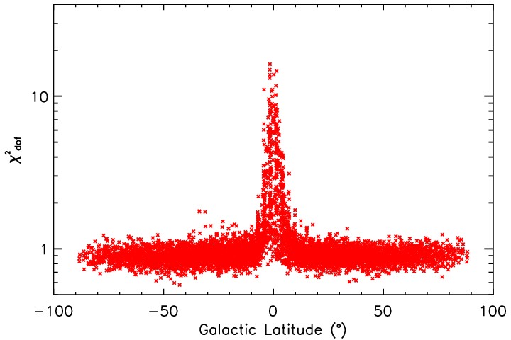
As an example, Fig. 2 presents as a function of Galactic latitude for the model. It shows that most fits at have and that fits at have a . Fig. 3 compares the distribution of at with the distribution of for the entire sky. That both distributions are well approximated by a Gaussian indicates that the fits don’t have a significant systematic bias. The widths of the distributions are as expected ( 0.1) for a distribution of random data with 210 degrees of freedom. That the distributions center at 0.93 means that statistical errors of the data are slightly overestimated by , and that the cutoff is really at with a probability of . Because the uncertainties of the FIRAS data include some systematic effects, we do not feel at liberty to reduce the uncertainty. Based on the cut, the model is a good fit to the data for over 87 per cent of the full sky area and is rejected by the data at the Galactic plane.
Readers interested in the best-fitting parameters (, , [C II] and [N II] intensities), their uncertainties and correlations for each of the aforementioned models are referred to Liang (2011).

4.2.2 Dependence of best-fitting parameters on the signal-to-noise of data
Figs. 4 and 5 present , and of the best-fitting models for two spectra: one has high signal-to-noise (HSN) and is at a low Galactic latitude; the other one has low signal-to-noise (LSN) and is at a high Galactic latitude. For both cases, plots of vs. show that models with a wide range of different values can fit the data well. In the HSN case, a curve fit to as a function of is a concave up parabola, with the minimum at . The difference between at and that at is . At 210 degrees of freedom, this means a of , a 2-sigma difference. In the LSN case, the best-fitting curve to vs. is a much flatter parabola over with the minimum at . The difference between at and is .
Although models with different have only a small difference in , the best-fitting and are different significantly in the HSN case: At , the best-fitting dust temperature is K, compared to K at . This difference in temperature is larger than the sum of their errors. Similarly, the difference in of the two models is larger than the sum of their errors. On the contrary, in the LSN case, the difference in the best-fitting and of and models are well within the uncertainties of the respective parameters.
These results demonstrate the sensitivity of the fits to measurement errors. The existence of measurement noise inevitably causes a high degree of degeneracy between emissivity spectral index and dust temperature in the fits. While it is difficult to break this degeneracy, high signal-to-noise data help. Fitting data with high signal-to-noise results in well constrained parameters, which means that the choice of an model can cause statistically significant differences in the predictions of these parameters. On the other hand, fitting low signal-to-noise spectra results in small difference in and large error bars of the best-fitting parameters. The results cannot be used to differentiate models with different fixed values of . This is demonstrated in Fig. 6, which shows that the 68 and 95 per cent confidence contours of a HSN fit enclose much smaller regions in the - space than those of a LSN fit.
Figs. 7 shows sky maps of and that correspond to the minimum- model among all models tested at each pixel. Both maps show greater consistency in value at low latitudes and more fluctuations around the Galactic poles. That consistent values appear in the region surrounding the Inner Galaxy is reasonable because star formation as the most important heat source for dust takes place in the Galactic disk and at the bulge. That large fluctuations appear near the poles, on the other hand, has to do with lower signal-to-noise data in these regions compared to those measured at lower latitudes. This happens because few dust grains exist at high latitudes, and they do not emit as strongly as those close to the Galactic disk.


 |
 |
Since low signal-to-noise data cannot give adequate constraint to model parameters and exacerbates the degeneracy between dust temperature and spectral index, in order to construct the best dust model, we need to find ways to increase the signal-to-noise of the data.
4.3 Fitting averaged spectra of different-size sky regions
Taking average of the high-latitude spectra based on latitudinal or longitudinal divisions of the sky can tighten the constraint on model parameters. However, such divisions are based on our expectations of the distribution of Galactic dust. They are not optimal because our knowledge of the dust distribution is incomplete. In our experiments (Liang, 2011), of regional fits are much higher than of fits to the individual spectra that comprise the regional averages. Since larger sky regions include different types of dust emission spectra, the steep increase in value means that the averaging has achieved a sufficient signal-to-noise ratio and that spectral variation has become statistically important. In order to preserve information on spectral variation in the model, the amount of spatial averaging needs to reflect the signal-to-noise of the data.
One way to do this is to base the amount of spectral averaging on signal-to-noise of the averaged spectrum. Starting with the base level, where a pixel’s own spectrum is used to fit a model, if the fit does not give well constrained parameters due to inadequate signal-to-noise, the procedure goes on to fit the average of the original spectrum and its eight immediate neighbors. This process of involving more of the adjacent spectra to form a new average goes on until the derived parameters are sufficiently constrained. In this way, results from fits done at the base level have a spatial resolution of 6.71 . At the next level, results have a spatial resolution of 60.37 , and so on.
4.3.1 constraint on fixed- models
 |
 |
All-sky one-component fixed- models with in the range and lower limit of at 5, 10, 20 and 40 are obtained separately. In general, one-component fixed- models with different lower limits on the values can fit most spectra except those at the Galactic plane. A more restricted lower limit on the values requires a greater amount of spatial averaging. As dust spectra with refined differences in shape are binned together and the uncertainties of the averaged spectrum are reduced, we subject the comparison between the averaged spectrum and the modified blackbody function to an increasingly restricted standard. The result is a steep increase in value. The lower plot of Fig. 8 demonstrates this relation by plotting as a function of Galactic latitude for the case of . Note that of high-latitude () fits move from to as lower limit on starts with none and increases to 40.
Histograms of the all-sky collections of for different limits on are presented in the upper plot of Fig. 8. For the case of 5, 10 and 20, the three histograms have the shape of a Gaussian, peak at 0.93, 0.94 and 0.96 respectively, and all have a width of 0.10. At 40 the histogram peaks at 1.00, has a width of 0.12, and a thick tail in the range . This means that at the level of 40, it is no longer adequate to use a modified blackbody function to describe variations in the dust spectral shape.
Imposing a more stringent limit on leads to a variety of spatial resolutions in each all-sky collection of fits. A more stringent requirement on means lower spatial resolutions for fits at high latitudes. For the one-component model with , only 0.59 per cent of the total sky area require fits with a 60.37 resolution instead of the default 6.71 . For a 10 per cent constraint on , 0.47 per cent area of the full sky require fits to be at 167.70 resolution, 7.24 per cent at 60.37 resolution, and the rest at 6.71 resolution. A balance between having adequate constraint on parameters, preserving as many valid models as possible, and keeping regional sizes low can be achieved at the 10 level.
A plot of distributions for 13 all-sky fixed- models with in the range at 0.1 increment and is presented in Fig. 9. The high- tails of these distributions show that models with the largest (2.6) and smallest (1.4) values of have more fits with large . The plot of excess for these all-sky models is presented in Fig. 9. It shows that the all-sky model can fit the largest amount of data (87.6 per cent area of the full sky). Fig. 10 presents sky maps of , spatial resolution, dust temperature, optical depth, and the signal-to-noise of parameters from fitting the one-component model. Each of the 6063 fits presented there satisfies the requirement with the least amount of spatial averaging. In the parameter maps, if a fit has less than 10 per cent probability (i.e., ), then its corresponding pixel is masked in white. Fit results for other models at different levels of constraint on are provided in Liang (2011).
 |
 |
One-component fits with
 |
 |
 |
 |
 |
 |
4.3.2 constraint on a free- model
We apply a similar strategy to constrain fits that use a free- model. Instead of focusing on the signal-to-noise of the dust temperature, we now use signal-to-noise of the emissivity spectral index to gauge the amount of spectral averaging. As an example, sky maps of the best-fitting parameters and their signal-to-noise for the free- model with are presented in Fig. 11.
One-component free- fits with
 |
 |
 |
 |
 |
 |
 |
 |
| Level | Regional size of fits | Percentage of the full sky at a regional average | ||
|---|---|---|---|---|
| () | ||||
| 1 | 6.71 | 40.01 | 30.63 | 22.09 |
| 2 | 60.43 | 23.14 | 24.53 | 22.51 |
| 3 | 167.86 | 11.87 | 11.07 | 10.60 |
| 4 | 329.00 | 4.61 | 8.59 | 6.41 |
| 5 | 543.86 | 3.53 | 3.48 | 5.53 |
| 6 | 812.44 | 2.18 | 2.78 | 4.62 |
| 7 | 1134.73 | 1.01 | 2.12 | 3.30 |
| 8 | 1510.73 | 1.92 | 2.59 | |
| 9 | 1940.45 | 1.22 | 2.23 | |
| 10 | 2423.88 | 2.08 | ||
| 11 | 2961.03 | 1.90 | ||
| 12 | 3551.89 | 1.53 | ||
| 13 | 4196.47 | 0.72 | ||
| 14 | 4894.76 | 0.23 | ||
| Total | 87.66 | 87.19 | 86.34 | |
Notice that with spatial averaging the dust temperature map has more consistent values at high latitudes near the Galactic poles than that obtained from the 7∘-pixel fits in Fig. 7. The uncertainty of is less than 7.4 per cent as a result of the constraint on , and the uncertainty of has a maximum of 23.25 per cent. The spatial resolution of these fits are presented in an all-sky map in Fig. 11 and summarized in Table 2.
The upper panel in Fig. 12 compares distributions of fits that use no constraint on any parameter and those that satisfy 5.0, 6.7, and 10.0. The shape of the distributions again resemble a Gaussian, and the constrained distributions all centre around 0.95. This means that there is no apparent systematic bias in the fits and the error estimates for the data is about right.
The plot of vs. Galactic latitude, lower panel of Fig. 12, shows that at , continues to be as is the case of fitting all-sky one-component fixed- models. At high latitudes, do not flare up with increasing constraint on , as oppose to that which happens when requirements are imposed on a fixed- model.
Fig. 13 presents distributions of and of one-component free- fits that use no constraint on any parameter and those that satisfy 5.0, 6.7, and 10.0. The centres of the distributions are at 1.80, 1.83, 1.85, and 1.88, respectively. This plot shows that the requirement has the effect of moving from below 1.5 to higher values. With even a moderate amount of constraint on , the range of values quickly reduces to between 1 and 3, an indication that values outside this range are rare in nature.
Also shown in Fig. 13, the distributions do not peak at a single value. Instead, there is a range of most popular temperatures between 17 and 20 K. Compared to the unconstrained case, the requirement smooths out the high-temperature points and effectively replaces them with values at or below 20 K.
| Constraint on | |||
|---|---|---|---|
| (K) | (K) | ||
| min | max | ||
| 10.11 | 23.83 | 2.67 | |
| 10.12 | 22.69 | 1.95 | |
| 13.69 | 22.69 | 1.26 | |
| Constraint on | |||
| min | max | ||
| 1.08 | 4.71 | 0.91 | |
| 1.08 | 4.80 | 0.71 | |
| 1.24 | 3.13 | 0.31 | |
| Constraint on | |||
| (per cent) | |||
| min | max | ||
| 0.33 | 46.15 | 62.83 | |
| 0.45 | 46.15 | 49.02 | |
| 0.61 | 46.15 | 23.25 | |
The amounts of constraint on dust temperature, optical depth and emissivity spectral index for various levels of constraint on are summarized in Table 3. In order to place adequate constraint on each parameter and to keep the regional sizes low, we adopt the constraint as our standard.


5 Discussion
5.1 Dust temperature at high Galactic latitudes
Dust temperature is not measured directly in astronomical observations. Instead, one derives dust temperature from intensity measurements of dust emission and a model that describes the emission process. That dust temperature decreases with the increase in Galactic latitude is supported by observations which identify thermal dust to be the origin of the Galaxy’s diffuse emission, observations which show that the diffuse emission decreases from low to high Galactic latitudes following a cosecant law, observations of the cosecant law for dust reddening and extinction in the Galaxy with respect to Galactic latitude, and observations of the decreasing number of bright stars toward the Galactic polar caps. Substantial amount of work has been carried out over the last four decades, we mention only a few as examples:
In reviewing global properties of dust in the Galaxy, Stein & Soifer (1983) point out that “the far-infrared luminosity in the Galaxy is associated with regions where stars are now or were recently forming,” and so “even in the galactic center region, much of the far-infrared luminosity is associated with ongoing or recent star formation activity.” Using far-infrared luminosity as a measure of the current rate of star formation, dust acts as “a frequency converter which absorbs the short wavelength photons emitted by the newly formed stars and re-emitting the energy at far-infrared wavelengths.”
That dust grains are heated by the general interstellar radiation field (ISRF) which follows a cosecant law to the Galactic poles and has a stellar origin have been confirmed by many research groups. For instance, by fitting spectra of diffuse emission from the Galactic plane Mezger et al. (1982) and Mathis et al. (1983) identify two main contributors to the diffuse emission at wavelengths m: dust heated by O stars (60%) and dust associated with diffuse atomic intercloud gas heated by the general interstellar radiation field (40%). They conclude that dust associated with clouds containing no luminous sources of heating such as OB stars contributes less than 7% of the total diffuse far-infrared/sub-millimeter emission. In 1986, Cox, Krüegel & Mezger showed that the total luminosity of the re-radiated dust emission from the Galactic disk is about 40% of the total stellar luminosity. Their best-fitting dust model predicts that 90% of the total Galactic infrared luminosity come from three components: a cold dust ( K) component associated with atomic hydrogen, a very cold dust ( K) component associated with molecular hydrogen and located inside quiescent molecular clouds, and a warm dust ( K) component associated with ionized gas in extended low density HII regions heated by O and B stars. The first two components are heated by the general ISRF generated by both young and old stellar populations. They dominate the sub-millimeter part of the spectrum and have a total luminosity of of the total Galactic infrared luminosity. The luminosity of the warm dust component, on the other hand, accounts for of the total Galactic IR luminosity. Using the first all-sky infrared measurements taken by the Infrared Astronomical Satellite (IRAS, IRAS Explanatory Supplement (1988)), Boulanger & Pérault (1988) show that Galactic emission exists at Galactic latitude at 12, 25, 60 and 100 m and that the emission comes mainly from dust heated by the ISRF associated with atomic gas and diffuse ionized gas. More specifically, they show that the Galactic latitude profiles of the IRAS all-sky measurements at 60 and 100 m follow a cosecant law from 10∘ to the poles. This means that dust emission decreases from low to high latitudes in the manner as would be expected for a plane-parallel configuration.
Not only does the strength of the ISRF decreases with increasing latitude, but the amount of dust at high Galactic latitudes also decreases following a cosecant law. Distribution of dust at high Galactic latitudes can be inferred from studies of dust reddening and extinction. For example, McClure & Crawford (1971) use 207 late-type stars (K giants) near the north Galactic pole to calculate a reddening law and find that it is consistent with the cosecant law (), where the Sun is assumed to be in a cylindrical hole of an absorbing layer in the Galactic plane. They conclude that there is almost no absorption from the pole down to 50∘. de Vaucouleurs & Buta (1983) studies high-latitude extinction in extragalactic objects using five independent methods: counts of faint galaxies, counts of distant galaxy clusters, mean surface brightness of bright galaxies, hydrogen-luminosity ratio measured by the HI index for bright galaxies, and total color indices of bright galaxies. They show that extinction derived from each of these methods supports the cosecant law from to the poles in each Galactic hemisphere.
Finally, we know that stars are the power houses in the Galaxy for both the ISRF and interstellar dust grains and that all-sky surveys have shown that the Galactic polar regions have fewer and cooler stars (sky maps in IRAS Explanatory Supplement 1988; Arendt et al. 1998; Voges et al. 1999; Gudennavar et al. 2012). With the observations of less intense emission, fewer dust particles and fewer sources of energy at the Galactic polar regions, we thus expect that dust temperature in those regions to be lower accordingly.
5.2 Comparing dust temperature predictions of different models
The crucial test to any model is comparison with observations. In this section, we present all-sky maps of dust temperature obtained from the literature and those from our study. We argue that since dust temperature distribution should generally decrease with the increase in Galactic latitude, models that fail such a test are unphysical.
 |
 |
 |
 |
 |
 |
Fig. 14 presents dust temperature predictions by the two-component model of Reach et al. (1995), the two-component and Model #8 of Finkbeiner et al. (1999), the one-component model with , and the one-component free- model with . The last two models are the ones derived in Section 4. We do not have Planck Collaboration’s dust temperature predictions (Planck Collaboration, 2011a), but since their one-component dust model has the emissivity spectral index at 1.8, we use the temperature map of our one-component model to approximate their results.
Notice the difference in dust temperature predictions at the Galactic polar caps relative to lower latitude regions in these maps. In the first three cases, where emissivity spectral indices of the models are fixed, temperature estimates around the Galactic polar caps are noticeably higher or at about the same level compared to those at lower latitudes. On the other hand, the free- model predicts the polar caps to have the lowest temperature of the entire Galaxy.

To perform the comparison in a more quantitative manner, we plot vs. Galactic latitude for the different models in Fig. 15. One may notice that data points corresponding to the one-component model flare up at most dramatically among all models. One may also notice that the two temperature components of Model #8 share the same distributions and that their values are approximately independent of Galactic latitude. In the southern hemisphere, one may notice that the two dust components of the Reach model consistently have higher temperatures at the Galactic polar caps than at mid latitudes. In fact, temperature of the cold dust at the southern polar cap is the highest that cold dust experiences throughout the entire Galaxy. In comparison to these three models, the free- model is the only model which predicts a decrease in dust temperature with respect to Galactic latitude.

We investigate the possibility that dust temperature predictions are biased positively when signal-to-noise of data decreases. Fig. 16 plots as a function of as given by the two-component model of Reach et al. (1995), the one-component model, and the one-component free- model. Model #8 is not included because FDS study does not provide error estimates for their models. Notice that while signal-to-noise of the fits vary by over one, sometimes two, order of magnitude, values change by less than 70 per cent, so is approximately independent of the signal-to-noise of the fits. More specifically, within the set of points for each model, in comparison to the (, ) pairs, the existence of lower and lower pairs or higher and higher pairs shows that the data do not support a definitive causal relation between low signal-to-noise and high temperature prediction. Based on these observations, we conclude that any potential bias to the fits due to low signal-to-noise cannot be the main reason for high temperature predictions seen at the Galactic polar caps by fixed- models.
Since we have checked temperature predictions of models with spectral index at the range of most likely values between 1.4 and 2.6 (Liang, 2011), and they all exhibit higher temperature at the Galactic polar caps than at lower latitudes, we suspect that such a phenomenon is an inherent artifact resulted from fixing the emissivity spectral index at a particular value. As a result, we argue that the temperature predictions of these fixed- models are unphysical.
In addition to predicting reasonable temperature distribution at the Galactic polar caps, the free- model predicts regions with known heating sources to have higher temperature than their surrounding environment. For instance, we can identify, off the Galactic plane, high temperature regions that correspond to the Ophiuchus region, Centauri, the Large Magellanic Cloud and the Orion region. At the Galactic plane, model predictions show that dust temperature decreases with increasing Galactocentric distance, consistent with observations of the DIRBE experiment (Sodroski et al., 1994). On top of this temperature gradient the temperature map shows the Outer Galaxy to be asymmetrically interspersed with strong infrared emission regions, such as NGC 7538 at , Cas A at , W3/4/5 at , Cygnus region at , and the Gum Nebula at . These regions at the Outer Galaxy are currently masked under the criterion that of the fit be 1.13. For these regions we believe that complex emission sources in addition to thermal dust have contributed to our prepared spectra. This challenges our model’s assumption that only thermal dust can contribute to the continuous emission. If true, then our model is no longer sufficient.


Fig. 17 present samples of fits to the average dust spectra by each of the aforementioned models at different Galactic latitudes. While most models are able to simulate the data with various degrees of success, the free- model is consistently able to trace the data points closely at all Galactic latitudes. Fig. 18 compares the normalized difference between data and intensity predictions for the same set of models and the same sky regions. It shows that the free- model is able to match the data within 1-sigma for majority of the channels while the other models are less consistent at predicting close to measurement values across frequency and Galactic latitude. That the normalized differences of the model are comparable to those of the free- model demonstrates the limitation of relying on a single number to evaluate a multifaceted operation, such as using the normalized difference or the to differentiate models. Here, the free- model and the model have about the same value, but one of them has a strong connection with other facts we know of the Galaxy and the other does not.
5.3 Relation between dust temperature and emissivity spectral index
The existence of an anti-correlation between the emissivity spectral index and dust temperature has been a subject of debate in the last decade. For example, Veneziani et al. (2010) did not find a clear inverse correlation between the two parameters in BOOMERANG’s measurements of the Galactic cirrus. Planck Collaboration (2011a) derived all-sky dust temperature using a fixed value of the emissivity spectral index due to degeneracy between temperature and spectral index in a free- fit (Shetty et al., 2009a; Shetty et al., 2009b). And Planck Collaboration (2011c) carried out analysis of dust properties at high Galactic latitudes using the same fixed spectral index model in order to maintain consistency within the Collaboration.
On the other hand, Dupac et al. (2001); Dupac et al. (2002); Dupac et al. (2003) of the ProNaOS experiment reported evidence of the inverse correlation in their observations of M42, M17 and NGC891, Désert et al. (2008) of the Archeops experiment confirmed the correlation on 300 Galactic point sources, Paradis (2010) confirmed the existence of the correlation in two Hi-GAL fields at the Galactic plane, and Planck Collaboration (2011b) concluded that observation of objects in the Early Cold Core Catalogue were not consistent with a constant value of the spectral index over all temperature.
The strongest argument for the existence of a temperature dependent power-law emissivity spectral index comes from laboratory measurements. Agladze et al. (1996) measured absorption spectra of crystalline and amorphous silicate grains at 0.7 – 2.9 mm at 1.2 – 30 K and found that the wavelength dependent absorption coefficients of the amorphous grains can be modeled with power laws, and the exponents of which vary with temperature. Agladze et al. attributed the correlation to a two-level population effect found in the low-lying tunneling states in bulk glasses. Mennella et al. (1998) measured the absorption coefficients of crystalline and amorphous carbon and silicate grains at 20 m – 2 mm at 4 – 295 K and found that the absorption coefficient followed a power law with the spectral index depending on grain temperature. They attributed the observed pattern to the dominance of two-phonon difference processes. In 2001, Chihara et al. measured far-infrared absorption spectra of crystalline circumstellar dust analogues between 20 – 80 m at 4.2 K and at 295 K. They also reported a higher value of the spectral index at 4.2 K than at 295 K. In 2005, Boudet et al. measured the mass absorption coefficients of amorphous silicates between 100 m – 2 mm at 10 – 30 K and found that the power law spectral index had a strong temperature and wavelength dependence. More specifically, the anti-correlation between spectral index and grain temperature was more pronounced at 500 m – 1 mm than at 100 – 250 m. Comparing their measurements with the temperature-spectral index relation deduced from synthesis of the ProNaSO observations, Boudet et al. found a comparable anti-correlation between temperature and spectral index between observations and laboratory measurements when the spectral index is between 1 and 2.7. They attributed the origin of the relation to the tunneling processes in two level systems. Bringing together evidence from laboratory measurements and astronomical observations, Meny et al. (2007) proposed a model that relates the emission spectrum’s dependence on temperature and internal structure of the grains. Additional evidence in support of the explanation that internal grain structures give rise to the apparent correlation between dust temperature and spectral index came in when Coupeaud et al. (2011) reported that mass absorption coefficients of synthesized analogues of interstellar amorphous silicate grains decreased with temperature and that the local spectral index anti-correlated with grain temperature. These laboratory results strengthen our confidence that the anti-correlation between dust temperature and spectral index seen in astronomical observations is not spurious but instead grounded on the physical properties of interstellar dust grains.
To test the possibility of an inverse correlation between emissivity spectral index and dust temperature in our data, we fit the best-fitting and values of the free- model with to the hyperbolic function and obtain and with a . Fig. 19 presents the data and the - relations identified by this and other works. Notice that our best-fitting - relation overlaps with all but that of the Hi-GAL field at . Since the (, ) pairs we used to constrain the hyperbolic function come from all over the sky except for about 13 per cent of the total sky area in the Inner Galaxy, the overlap with other experiments’ results confirms that our - correlation has a broad representation. That it is within one-sigma of the - relation identified in Paradis (2010) for the field may have to do with one or both of the following reasons. First, the physical properties of dust may have changed from the Inner Galaxy to regions far away from active star formation. If so, then our set of (, ) values is not a good representation of dust properties in the field since fits of the Inner Galactic spectra are not included. Secondly, one may understand the isolation of the curve for Hi-GAL field at from explanation given in Paradis (2010), which points to the fact that data from the field challenge their model’s single-temperature assumption. Finally, that our set of (, ) values marginally overlap with the relation from the Planck study of cold cores in the Galaxy (Planck Collaboration, 2011b) may have to do with the fact that there is only a small overlap between the two data sets: While the 7608 cold cores in the Planck Collaboration (2011b) analysis largely distribute along the Galactic plane, our model’s target regions are at mid and high latitudes and part of the Outer Galaxy. In addition, the 7608 cold cores form a selective group of objects. To be selected, an object has to be a compact source colder than the surrounding envelope and a 17-K diffuse Galactic background. This last criterion would have excluded over 73 per cent of our data points. Fig. 20 presents the constant contours, corresponding to confidence intervals with 68, 95 and 99.99 per cent probability. It shows that a temperature independent model is rejected by the data with more than 99.99 per cent probability, an indication for a real dependence between and .
We present a summary of the best-fitting and for other levels of constraint on the fits in Table 4. The exact functional form of the temperature-dependent spectral index cannot be established by our data alone. However, that a physically sensible fit to the all-sky data requires a free- model and that an inverse relation fits the and values well give strong support to the anti-correlation between the emissivity spectral index and dust temperature.
| constraint on fits | number of data points | |||
|---|---|---|---|---|
| no constraint | 5421 | 0.72 | ||
| 5386 | 0.83 | |||
| 5357 | 0.88 | |||
| 5305 | 0.99 |


The observed correlation between emissivity spectral index and dust temperature in our data is likely to be intrinsic rather than from noise. In 2009, Shetty et al. showed that the accuracy of parameter estimation depends on the wavelength range of the spectra used in model fitting. They show that for dust temperature K, fits using spectra at m are not sensitive to noise. However, if 40 K K, a 5 per cent noise in a data set of different and the same may generate a pattern in the best-fitting vs. plot that can be confused with a true anti-correlation in the two parameters. Since our spectra, coming at m, well sample the Rayleigh-Jeans tail of the peak of the K modified blackbody spectrum, our best-fitting parameters are good approximates of the true values.
As the quality of data improves, the free- model will allow future studies to pinpoint the values of and with greater accuracy. In Fig. 21 we present vs. of the all-sky collections of fits with different amounts of constraint on . It shows that the uncertainty in and are directly proportional while is more susceptible to errors than . That is, with more sensitive data one will be able to reduce uncertainty in and at the same time.
6 Conclusions
We have examined models of interstellar dust thermal emission at far-infrared and millimeter wavelengths. Starting with deducing a new and improved version of dust spectra from FIRAS calibrated measurements and unifying them with measurements of the DIRBE and the WMAP, one-component dust models with fixed and variable emissivity spectral index are fit to 6063 214-channel spectra at fixed and variable spatial resolutions.
We show that the free- model can predict more physically motivated dust temperature than models with fixed emissivity spectral index. With observations showing that the intensity of dust emission and the amount of dust decrease with the increase in Galactic latitude and that fewer and weaker stars exist at higher Galactic latitudes, dust temperature is expected to be lower at the Galactic polar caps than at lower latitudes. Among all-sky dust models found in the literature and the one-component dust models constructed in our study, we demonstrate that only the free- model passes this test. All fixed- models predict higher or the same temperatures at the Galactic polar caps as at lower latitudes.
Our best dust model is the one-component free- model with . It fits dust spectra over 86 per cent area of the full sky. Dust temperature is predicted to be () K, emissivity spectral index to be (), and optical depth to range at GHz (m) with a 23.25 per cent uncertainty. Our model has the 7∘ angular resolution of FIRAS and uses variable spatial averaging at high latitudes. It supports the interpretation of an anti-correlation between emissivity spectral index and dust temperature. We fit the relation to the and values and obtained and . A temperature independent model () is rejected by the data with more than 99.99 per cent probability, an indication that a real dependence between and .
The free- model can be used to remove dust contamination in CMB measurements. It can also serve as an all-sky extended-frequency-range reference for other experiments. With higher resolution data sets, such as those from Planck, one will be able to further refine our knowledge of interstellar dust grains and their interaction with other constituents in the Galaxy.
Acknowledgments
Some of the results in this paper have been derived using the HEALPix (K.M. Górski et al., 2005, ApJ, 622, p759) package.
We thank the anonymous reviewer for many invaluable suggestions which help improve the quality of this manuscript. ZL thanks Professor Charles Bennett for enlightening discussions, intuitive guidance and generous support, all of which made this work possible. ZL also thanks Drs. Janet Weiland, David Larson and Domenico Tocchini-Valentini for very helpful discussions.
References
- Agladze et al. (1996) Agladze N.I., Sievers A.J., Jones S.A., Burlitch J.M., Beckwith S.V.W., 1996, ApJ, 462, 1026
- Arendt et al. (1998) Arendt R.G. et al., 1998, ApJ, 508, 74
- Bennett et al. (2003a) Bennett C.L. et al., 2003a, ApJ, 583, 1.
- Bennett et al. (2003b) Bennett C.L. et al., 2003b, ApJS, 148, 97
- Boggess et al. (1992) Boggess N.W. et al., 1992, ApJ, 397, 420
- Boudet et al. (2005) Boudet N. et al., 2005, ApJ, 633, 272
- Boulanger & Pérault (1988) Boulanger F., Pérault M., 1988, ApJ, 330, 964
- Boulanger et al. (1996) Boulanger F., Abergel A., Bernard J.P., Burton W.B., Desert F.X., Hartmann D., Lagache G., Puget J.L., 1996, A&A, 312, 256
- Calabretta & Greisen (2002) Calabretta M.R., Greisen E.W., 2002, A&A, 395, 1077-1122
- Calabretta & Roukema (2007) Calabretta M.R., Roukema B.F., 2007, MNRAS, 381, 865
- Chan & O’Neill (1975) Chan F.K., O’Neill E.M., 1975, EPRF Technical Report 2 - 75 (CSC). Computr Science Corporation, Silver Springs, Maryland
- Chihara et al. (2001) Chihara H., Koike C., Tsuchiyama A., 2001, PASJ, 53, 243
- Coupeaud et al. (2011) Coupeaud A. et a., 2011, A&A, 535, A124
- Cox, Krüegel & Mezger (1986) Cox P., Krüegel E., Mezger P. G., 1986, A&A, 155, 380
- de Vaucouleurs & Buta (1983) de Vaucouleurs G., Buta R., 1983, AJ, 88, 939
- Désert et al. (2008) Désert F.X. et al., 2008, A&A, 481, 411
- DIRBE Explanatory Supplement (1998) COBE Diffuse Infrared Background Experiment (DIRBE) Explanatory Supplement. 1998, in Hauser M.G., Kelsall T., Leisawitz D., Weiland J., eds, COBE Ref. Pub. No. 98-A, Greenbelt, MD: NASA/GSFC
- Draine & Lee (1984) Draine B.T., Lee H.M., 1984, ApJ, 285, 89
- Dupac et al. (2001) Dupac X. et al., 2001, ApJ, 553, 604
- Dupac et al. (2002) Dupac X. et al., 2002, A&A, 392, 691
- Dupac et al. (2003) Dupac X. et al., 2003, A&A, 404, L11
- Finkbeiner et al. (1999) Finkbeiner D.P., Davis M., Schlegel D.J., 1999, ApJ, 524, 867
- Finkbeiner et al. (2000) Finkbeiner D.P., Davis M., Schlegel D.J., 2000, ApJ, 544, 81
- FIRAS Explanatory Supplement (1997) COBE Far Infrared Absolute Spectrophotometer (FIRAS) Explanatory Supplement. 1997, in Brodd S., Fixsen D.J., Jensen K.A., Mather J.C., Shafer R.A., eds, COBE Ref. Pub. No. 97-C. Greenbelt, MD: NASA/GSFC
- Fixsen (2009) Fixsen D.J., 2009, ApJ, 707, 916
- Fixsen & Dwek (2002) Fixsen D.J., Dwek, E., 2002, ApJ, 578, 1009
- Fixsen & Mather (2002) Fixsen D.J., Mather J.C., 2002, ApJ, 581, 817
- Fixsen et al. (1994a) Fixsen D.J. et al., 1994a, ApJ, 420, 445
- Fixsen et al. (1994b) Fixsen D.J. et al., 1994b, ApJ, 420, 457
- Fixsen et al. (1996) Fixsen D.J., Cheng E.S., Gales J.M., Mather J.C., Shafer R.A., Wright E.L., 1996, ApJ, 473, 576
- Fixsen et al. (1997b) Fixsen D.J. et al., 1997b, ApJ, 490, 482
- Fixsen et al. (1998) Fixsen D.J., Dwek E., Mather J.C., Bennett C.L., Shafer R.A., 1998, ApJ, 508, 123
- Gold et al. (2009) Gold B. et al., 2009, ApJS, 180, 265
- Gorjian et al. (2000) Gorjian V., Wright E.L., Chary R.R., 2000, ApJ, 536, 550
- Górski et al. (1999) Górski K.M., Hivon E., Wandelt B.D., 1999, in Banday A.J., Sheth R.S., Da Costa L., eds, Proceedings of the MPA/ESO Cosmology Conference, Evolution of Large-Scale Structure. Ipskamp, NL, 37
- Górski et al. (2005) Górski K.M., Hivon E., Banday A.J., Wandelt B.D., Hansen F.K., Reinecke M., Bartelmann M., 2005, ApJ, 622, 759
- Gudennavar et al. (2012) Gudennavar S.B., Bubbly S.G., Preethi K., Murthy J., 2012, ApJS, 199, 8
- Hauser et al. (1998) Hauser M.G. et al., 1998, ApJ, 508, 25
- Hill et al. (2009) Hill R.S. et al., 2009, ApJS, 180, 246
- Hinshaw et al. (2003) Hinshaw G. et al., 2003, ApJS, 148, 63
- Hinshaw et al. (2007) Hinshaw G. et al., 2007, ApJS, 170, 288
- Hinshaw et al. (2009) Hinshaw G. et al., 2009, ApJS, 180, 225
- IRAS Explanatory Supplement (1988) IRAS Catalogs and Atlases: Explanatory Supplement. 1988, in Beichman C.A., Neugebauer G., Habing H.J., Clegg P.E., Chester T.J., eds, Washington, DC: GPO.
- Jarosik et al. (2003) Jarosik N. et al., 2003, ApJS, 145, 413
- Jarosik et al. (2007) Jarosik N. et al., 2007, ApJS, 170, 263
- Jones et al. (2002) Jones L.V., Elston R.J., Hunter D.A., 2002, ApJ, 124, 2548
- Kelsall et al. (1998) Kelsall T. et al., 1998, ApJ, 508, 44
- Lagache et al. (1998) Lagache G., Abergel A., Boulanger F., Puget J.L., 1998, A&A, 333, 709
- Lagache et al. (2000) Lagache G., Haffner L.M., Reynolds R.J., Tufte S.L., 2000, A&A, 354, 247
- Liang (2011) Liang Z., 2011, PhD thesis, Johns Hopkins University, http://gradworks.umi.com/34/92/3492589.html
- Mather (1982) Mather J.C., 1982, Opt. Eng., 21, 769
- Mather et al. (1986) Mather J.C., Toral M. & Hemmati H. 1986, Appl. Opt., 25, 2826
- Mather et al. (1990) Mather J.C. et al., 1990, ApJ, 354, L37
- Mather et al. (1993) Mather J.C., Fixsen D.J. & Shafer R.A., 1993, Proc. SPIE, 2019, 168
- Mather et al. (1994) Mather J.C. et al., 1994, ApJ, 420, 439
- Mather et al. (1999) Mather J.C., Fixsen D.J., Shafer R.A., Mosier C., Wilkinson D.T., 1999, ApJ, 512, 511
- Mathis et al. (1983) Mathis J. S., Mezger P. G., Panagia N., 1983, A&A, 128, 212
- McClure & Crawford (1971) McClure R.D., Crawford D.L., 1971, AJ, 76, 31
- Mennella et al. (1998) Mennella V., Brucato J.R., Colangeli L., Palumbo P., Rotundi A., Bussoletti E., 1998, ApJ, 496, 1058
- Meny et al. (2007) Meny C., Gromov V., Boudet N., Bernard J.P., Paradis, D., Nayral C., 2007, A&A, 468, 171
- Mezger (1986) Mezger P.G., 1986, Astrophys. & Space Sci., 128, 111
- Mezger et al. (1982) Mezger P.G., Mathis J.S., Panagia N., 1982, A&A, 105, 372
- O’Neill & Laubscher (1976) O’Neill E.M., Laubscher R.E., 1976, NEPRF Technical Report 3 - 76 (CSC). Computer Sciences Corportion, Silver Springs, Maryland
- Page et al. (2003) Page L. et al., 2003, ApJS, 148, 39
- Paradis (2010) Paradis D. et al., 2010, A&A, 520, 8
- Planck Collaboration (2011a) Planck Collaboration, 2011a, A&A, 536, 19
- Planck Collaboration (2011b) Planck Collaboration, 2011b, A&A, 536, 23
- Planck Collaboration (2011c) Planck Collaboration, 2011c, A&A, 536, 24
- Reach et al. (1995) Reach W.T. et al., 1995, ApJ, 451, 188
- Schlegel et al. (1998) Schlegel D.J., Finkbeiner D.P., Davis, M., 1998, ApJ, 500, 525
- Shetty et al. (2009a) Shetty R., Kauffmann J., Schnee S., Goodman A.A., 2009, ApJ, 696, 676
- Shetty et al. (2009b) Shetty R., Kauffmann J., Schnee S., Goodman A.A., Ercolano B., 2009, ApJ, 696, 2234
- Silverberg et al. (1993) Silverberg R.F., Hauser M.G., Boggess N.W., Kelsall T.J., Moseley S.H., Murdock T.L., 1993, Proc. SPIE, 2019, 180
- Sodroski et al. (1994) Sodroski T.J. et al., 1994, ApJ, 428, 638
- Stein & Soifer (1983) Stein W.A., Soifer B.T., 1983, ARA&A, 21, 177
- Veneziani et al. (2010) Veneziani M. et al., 2010, ApJ, 713, 959
- Voges et al. (1999) Voges W. et al., 1999, A&A, 349, 389
- White & Stemwedel (1992) White R.A., Stemwedel S.W., 1992, ASPC, 25, 379
- WMAP Five-Year Explanatory Supplement (2008) Wilkinson Microwave Anisotropy Probe WMAP: Five-Year Explanatory Supplement. 2008, in Limon M. et al., eds, Greenbelt, MD:NASA/GSFC
- Wright et al. (1991) Wright E.L. et al., 1991, ApJ, 381, 200