New Approach to Continuum Path Integrals for Particles and Fields

It is quantum physics which dominates microscopic phenomena less than the atomic scale [1]. One elegant way to describe the quantum phenomena is the path integral method developed by Feynman [2], in which all possible paths are taken into account with the probability amplitude $\exp(iS/\hbar)$ with $S$ the action of the system. The path integral method gives a clear interpretation of behavior of particles in quantum mechanics as fluctuations from the classical paths, although exact evaluations of the path integrals are possible only in few cases such as the harmonic oscillator [3]. The path integral method also promotes modern developments of theoretical elementary particle physics and supplies a nonperturbative technique for quantum field theories [4].

The evaluation of the path integrals can be simplified by discretizing time-space, in which derivations and integrations are replaced with finite differences and summations, respectively, and measure of the path integrals becomes a countable product. An important example of the discretized path integrals is the lattice QCD (quantum chromodynamics) [5], by which nonperturbative aspects of QCD have been revealed [6]. However, the time-space discretization explicitly breaks continuous symmetries of time-space such as the translational symmetry down to discrete symmetries, and sometimes leads to qualitative discrepancies such as magnetic monopoles in the lattice QED (quantum electrodynamics) [7]. Hence it is desired to perform the path integrals in continuous time-space from viewpoint of complementarity for the discretized approach.

In this paper we develop an approach to evaluating the continuum path integrals in Euclidean time ($t\to-i\tau$) for particles and fields. The continuous paths are described by sum of smooth functions with weight $\exp(-S)$ by the Metropolis method [8]. Here we take the natural units $\hbar=c=k_{\rm B}=1$.

Firstly, for a nonrelativistic particle with one degree of freedom $q$ in a periodic boundary condition with period ${\cal T}$, $q(\tau+{\cal T})=q(\tau)$, the path integral method evaluates the quantum transition amplitude in Euclidean time as [2],

Here the measure ${\cal D}q$ is formally defined as an uncountable product, and the expression (1) means that the quantum transition amplitude corresponds to the summation of all possible paths for the particle with the probability amplitude $\exp(-S)$. Since the quantum fluctuations of the particle are weighted with the factor $\exp(-S)$, an expectation value of an operator ${\cal O}[q]$ in quantum mechanics can be evaluated by using $N$ paths $q_{n}$ ($n=1,\,2,\,\cdots,\,N$) weighted with $\exp(-S)$ as,

where the last approximation becomes good for large $N$.

Before explaining our approach to the continuum path integrals, we briefly review the discretized approach to the path integrals for a nonrelativistic particle in the periodic boundary condition. In this case the particle position is represented as $\tilde{q}_{i}$ at time $\tilde{\tau}_{i}=ia$ with $i=1$, $\cdots$, $N_{\rm lat}$ and the lattice spacing $a\equiv{\cal T}/N_{\rm lat}$, and the path of the particle is obtained by connecting $\tilde{q}_{i}$ and $\tilde{q}_{i+1}$ from $i=1$ to $N_{\rm lat}$ with straight lines. Then measure of the path integral is defined as a countable product,

and the action is replaced with the corresponding discretized one, $\tilde{S}[\tilde{q}]$. The discretized path integrals are evaluated in the following way (see [9]). Namely, change of the particle position at each time $\tilde{\tau}_{i}$, $\delta\tilde{q}_{i}$, is generated as a random number within $[-\Delta,\,\Delta]$ with a fixed value $\Delta$, in which $\delta\tilde{q}_{i}$ has a property of the micro-reversibility. This change $\delta\tilde{q}_{i}$ is judged by the Metropolis test [8], in which $\tilde{q}_{i}+\delta\tilde{q}_{i}$ is redefined as $\tilde{q}_{i}$ in acceptance probability $\text{min}[1,\,\exp(\tilde{S}[\tilde{q}]-\tilde{S}[\tilde{q}+\delta\tilde{q}])]$ and otherwise $\delta\tilde{q}_{i}$ is rejected. We denote this step as $W_{i}$. Then the whole positions are updated by the “sweep”, i.e., performing $W_{i}$ from $i=1$ to $N_{\rm lat}$. After several sweeps quantum paths in equilibrium weighted with $\exp(-\tilde{S})$ are obtained.

Now let us make our procedure for the simulation of the continuum path integrals from analogy to the discretized approach. Our idea here is to connect the neighboring points for the particle positions by smooth lines rather than straight lines. In order to achieve this, we smear the particle position in the discretized approach $\tilde{q}_{i}$ with a Gauss function of width $\xi_{i}$ at time $\tau_{i}$,

for $i=1$ to $N_{\rm lat}$, where $\tau-\tau_{i}$ means to take time distance between $\tau$ and $\tau_{i}$ in the periodic boundary condition. Here ($q_{i}$, $\tau_{i}$, $\xi_{i}$) in the continuous approach corresponds to ($\tilde{q}_{i}$, $\tilde{\tau}_{i}$, $a$) in the discretized approach. With this smearing one can naturally connect the path with smooth lines rather than straight lines as,

where $N_{\rm sum}(=N_{\rm lat})$ is number of the summed terms. In this construction of the smooth path, as $q_{i}$ for each $i$ takes value in range $[-\Lambda,\,\Lambda]$ with a some cut-off $\Lambda$ according to Eq. (3), $q(\tau)$ at each time takes value in similar range $[-\Lambda^{\prime},\,\Lambda^{\prime}]$ with a cut-off $\Lambda^{\prime}$ similar to $\Lambda$, and the minimal scale of the fluctuation for $q(\tau)$ corresponds to $\xi_{i}$. The positions of the Gauss functions $\tau_{i}$ may take random values rather than values in same interval, $\tau_{i}=i{\cal T}/N_{\rm sum}$, as long as every time is equally treated without making any special time. The width of the Gauss function, or the scaling constant, $\xi_{i}$, is fixed so that $\xi_{i}$ does not depend on $\tau_{i}$, which prevents any special time. In this study we take two strategies for $\xi_{i}$; one is to generate $\xi_{i}$ randomly within $[\lambda_{\xi},\,\Lambda_{\xi}]$ in uniform probability with ultraviolet and infrared cut-offs $\lambda_{\xi}$ and $\Lambda_{\xi}$, respectively (random scale), and the other is to use a properly fixed value (fixed scale). Then the weight $\exp(-S)$ is given by the Metropolis method for $q_{i}$ as in the discretized approach. Namely, an additional fluctuation $\delta q_{i}$ with randomly chosen $i$ is randomly generated within $[-\Lambda_{q},\Lambda_{q}]$ in uniform probability, where $\Lambda_{q}$ is a cut-off for the fluctuation amplitude. Then the charge $\delta q_{i}$ with respect to $q_{i}$ is judged by the Metropolis test, in which $q_{i}+\delta q_{i}$ is redefined as $q_{j}$ in acceptance probability $\text{min}[1,\,\exp(S[q]-S[q+\delta q])]$ and otherwise $\delta q_{i}$ is rejected. We emphasize that the additional fluctuation $\delta q_{i}$ is micro-reversible without making any special directions in coordinate space.

Here we note that $q(\tau)$ in Eq. (5) cannot describe all possible paths, since the Gauss functions in Eq. (5) cannot be a complete set with respect to the smooth functions in the periodic boundary condition. Therefore, at this point our construction of paths is an approximation with respect to the complete paths required by the measure ${\cal D}q$. Nevertheless, we expect that most of the possible paths can be taken into account when value of $N_{\rm sum}$ is sufficiently large with large $\Lambda_{q}$, small $\lambda_{\xi}$, large $\Lambda_{\xi}$, and dense $\tau_{i}$, in which case distribution of the Gauss functions with various width is sufficiently dense. We also note that time uniformity may be broken when the time components $\tau_{i}$ take values in same interval, $\tau_{i}=i{\cal T}/N_{\rm sum}$, but we expect that the uniformity will restore if one considers sufficiently dense distribution of the Gauss functions.

Our procedure can be summarized as follows:

1. 1.

   Make an initial condition for the path (5) by determining constants ($q_{i}$, $\tau_{i}$, $\xi_{i}$) from $i=1$ to $N_{\rm sum}$ in the following manner. Namely, $\tau_{i}$ is generated within range $[0,\,{\cal T}]$ so as not to make any special time, and $\xi_{i}$ is randomly generated within $[\lambda_{\xi},\,\Lambda_{\xi}]$ in uniform probability or is fixed as a proper value. The coefficient $q_{i}$ is randomly generated within $[-\Lambda_{q},\,\Lambda_{q}]$ (hot start) or is taken to be zero for all $i$ (cold start).

2. 2.

   Randomly choose $i$ and generate $\delta q_{i}$ within $[-\Lambda_{q},\,\Lambda_{q}]$ in uniform probability so as to construct an additional fluctuation,

   $$\delta q(\tau)=\delta q_{i}\exp\left[-\frac{(\tau-\tau_{i})^{2}}{\xi_{i}^{2}}\right].$$

   (6)

3. 3.

   According to the Metropolis method [8], accept the additional fluctuation $\delta q$ in probability $\text{min}[1,\,\exp(S[q]-S[q+\delta q])]$. If and only if the additional fluctuation $\delta q$ is accepted, we redefine the path $q+\delta q$ as $q$ (or equivalently redefine the coefficient $q_{i}+\delta q_{i}$ as $q_{i}$).

4. 4.

   Iterate steps 2. and 3. until the action as well as other expectation values converge.

In this procedure, we eventually obtain a smooth path for the particle (5), which is weighted with $\exp(-S)$ due to the step 3. Generalization to the systems with $f$ degrees of freedom ($f\geq 2$) is obvious. Here we emphasize that the description of smooth fluctuations only by the finite terms of Gauss functions is an approximation.

Now let us examine our approach by investigating a harmonic oscillator in one dimension, which action is written as,

with $\dot{q}\equiv dq/d\tau$. Here we fix its mass and angular frequency as $m=\omega=1$, and we take the time range ${\cal T}=20$. We consider three simulation conditions; $N_{\rm sum}=50$, $\Lambda_{q}=3$, and the fixed scale with $\xi=1$ (A), $N_{\rm sum}=100$, $\Lambda_{q}=3$, and the random scale with $\lambda_{\xi}=0.2$ and $\Lambda_{\xi}=1$ (B), $N_{\rm sum}=200$, $\Lambda_{q}=3$, and the fixed scale with $\xi=0.2$ (C). For the initial condition we fix $\tau_{i}$ as $\tau_{i}=i{\cal T}/N_{\rm sum}$ and randomly generate $q_{i}$ within $[-\Lambda_{q},\Lambda_{q}]$ as a hot start. We prepare $N=400$ paths for the three conditions, respectively. Since temperature of the system $1/{\cal T}$ is much smaller than the excitation energy, the quantum fluctuations in this study will reflect the ground state of the harmonic oscillator.

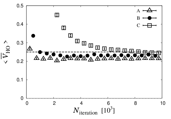As a result of the numerical simulation, quantum paths approach to equilibrium at around the iteration number, i.e., number of steps 2–3., $N_{\rm iteration}\approx 10^{3}$ for the condition A, $N_{\rm iteration}\approx 3\times 10^{3}$ for B, and $N_{\rm iteration}\approx 9\times 10^{3}$ for C. In Fig. 1 we show cooling behavior of the potential expectation value $V_{\rm HO}\equiv m\omega^{2}q^{2}/2$ in averaged form [$\overline{A}\equiv\int_{0}^{\cal T}d\tau A(\tau)/{\cal T}$] for the harmonic oscillator by the Metropolis method. As one can see, at the saturation point the potential expectation value reproduces the ground-state value ($=\omega/4$) with more than about $90\%$ accuracy in all conditions A, B, and C. Indeed, after iteration $N_{\rm iteration}=10^{4}$ the expectation value becomes $\langle\overline{V}_{\rm HO}\rangle=0.213\pm 0.04$ for the condition A, $0.237\pm 0.004$ for B, and $0.241\pm 0.004$ for C. The potential expectation value approaches to the ground-state value as the scale constant $\xi$ gets small and hence structures of the quantum fluctuations in fine scale can be described, which is similar to the case of the discretized approach. We expect that the accuracy of the potential expectation value will get higher if one uses even smaller $\xi$, although in which case large $N_{\rm sum}$, large $N_{\rm iteration}$, and large simulation time are required. We note that the expectation values are saturated with respect to $N_{\rm sum}$, namely we obtain same expectation values within range of statistical errors with larger $N_{\rm sum}$ in each conditions.

In order to see the quantum fluctuations in detail, we show in Fig. 2(upper) examples of the quantum fluctuations out of the $N=400$ paths. From the figure, in all conditions the paths fluctuate from the origin $q=0$ to their maximal amplitude $\sim\pm 1.5$. The mean squared radius of the fluctuation is $\langle\overline{q^{2}}\rangle=0.426\pm 0.08$ for the condition A, $0.474\pm 0.008$ for B, and $0.482\pm 0.008$ for C, which are close to the ground-state value $\langle q^{2}\rangle_{\rm GS}=0.5$ within smaller than about $10\%$ discrepancies. We note that in all conditions fluctuations in large scale are mainly composed of peak structures of width $\gtrsim 1$. Especially in the conditions B and C the fluctuation structures in large scale are described by sum of several Gauss functions, although they have small fluctuations in fine scale. Then let us visualize degree of the quantum fluctuations. For this purpose we make a histogram for $q$ with division of time range into sufficiently many parts in each path and then combine $N=400$ histograms to obtain the $q$-distribution $\rho_{q}$. The result is shown in Fig. 2(lower) together with the squared wave function of the ground state. As one can see, our $q$-distributions in all conditions behave consistently with the squared wave function. Especially it is interesting that behavior of the quantum fluctuations to large $q$ ($\sim\pm 3$) is very similar to the squared wave function.

In the examination of our approach for the harmonic oscillator, we have seen that our approach reproduces quantum behavior of the system with more than about $90\%$ accuracy by properly chosen scale constants, both in random and fixed scale cases. Especially, by using smaller scaling constant $\xi$, quantum behavior with higher accuracy is obtained.

Next let us apply our approach to relativistic field theories. It is important that our approach has possibilities to become a nonperturbative way to quantum field theories. To be specific, we firstly consider $\text{U}(1)$ gauge field $A_{\mu}(x)$ in four dimensions [$x=(\bm{x},\,\tau)$, $\mu=1$, $2$, $3$, $4$], and assume a periodic boundary condition with box size (${\cal X}$, ${\cal X}$, ${\cal X}$, ${\cal T}$). In a similar manner to the nonrelativistic particles, the quantum transition amplitude of the field in Euclidean time can be expressed as,

In the field path integrals, sole difference to the particle case is that the field is a function of four components of the coordinate $x$ rather than time $\tau$ only. Therefore, smooth quantum fields can be obtained by applying our approach (steps 1–4.) with an extension of $\tau\to x$. Then the field fluctuations are expressed as,

for each $\mu$, where $(x-x_{i_{\mu}})^{2}$ means to take squared distance between $x$ and $x_{i_{\mu}}$ in the periodic boundary condition.

Now let us evaluate quantum fluctuations of the $\text{U}(1)$ and $\text{SU}(2)$ gauge fields in four dimensions, which actions are,

with Lagrangian densities,

respectively. In this study we do not include gauge fixing terms nor the Faddeev-Popov ghosts in the Lagrangian densities. The $\text{SU}(2)$ gauge field has self-interactions with coupling $g$, for which we take $g=3.5$. In both $\text{U}(1)$ and $\text{SU}(2)$ gauge theories, we take the following simulation condition. Namely, we fix the coordinate $x_{i_{\mu(a)}}$ to be on sites of four-dimensional lattice $7^{3}\times 14$ dividing the box in same intervals with ${\cal T}=2{\cal X}$. We take the fixed scale with $\xi={\cal X}/(7\sqrt{\pi})={\cal T}/(14\sqrt{\pi})$. We note that $\xi$ corresponds to the minimal scale of quantum field theories, as the lattice spacing $a$ in the discretized framework. The cut-off for the fluctuation amplitude, $\Lambda_{A}$, is fixed as $\Lambda_{A}=1.3~\xi^{-1}$. At first of the iteration $A_{i_{\mu(a)}}$ is randomly generated as a hot start. We prepare $N=50$ paths for the $\text{U}(1)$ and $\text{SU}(2)$ gauge fields, respectively. During cooling by the Metropolis method, the action of the $\text{U}(1)$ [$\text{SU}(2)$] gauge field converges at around $N_{\rm iteration}\approx 3\times 10^{5}$ ($10^{6}$). It is interesting that at the saturation point $\langle\overline{\cal L}_{\text{SU}(2)}\rangle\approx 0.49~\xi^{-4}$ is smaller than $3\times\langle\overline{\cal L}_{\text{U}(1)}\rangle\approx 3\times 0.20~\xi^{-4}$ due to the self-interactions in $\text{SU}(2)$, where $\overline{\cal L}$ is averaged Lagrangian density [$\overline{\cal L}\equiv\int d^{4}x{\cal L}(x)/{\cal TX}^{3}$].

Quantum fluctuations of gauge fields provide a potential between (infinitely heavy) fundamental representation and its antiparticle, which can be evaluated through the Wilson loop of rectangle $C=T\times R$ defined as [5],

where ${\cal P}$ means to take the ordered exponential with the group generator $T^{a}$. We choose the gauge coupling for $\text{U}(1)$ as $g=0.303$ so that $\alpha\equiv g^{2}/(4\pi)\approx 1/137$. From the expectation values of the Wilson loop $\langle W\rangle$, the potential is evaluated as,

for sufficiently large $T$ and small $t$. In this study, in order to have enough statistics, we calculate average of $10$ Wilson loops at random positions in four-dimensional time-space for each set ($T$, $R$) in each path and then combine the results of $N=50$ paths. The results for $\text{U}(1)$ and $\text{SU}(2)$ gauge fields are shown in Fig. 3. As one can see, while the $\text{U}(1)$ gauge field qualitatively reproduces the Coulomb force, the potential from the $\text{SU}(2)$ gauge field shows confining linearity. A confining potential is the expected nonperturbative property of non-Abelian gauge theories inspired by the absence of free quarks in experiments [10], and our approach implies that quantization indeed generates confining field configurations in the $\text{SU}(2)$ gauge theory. Fitting our $\text{SU}(2)$ potential with $\sigma R+b$ we obtain the string tension $\sigma=0.17\pm 0.01~\xi^{-2}$, which brings a scale to the quantum $\text{SU}(2)$ gauge theory.

Here we should discuss the gauge symmetry in our approach. In the path integral formulations of gauge theories without gauge fixing terms nor Faddeev-Popov ghosts, the measure ${\cal D}A$ and the Lagrangian ${\cal L}$ are respectively gauge invariant. This indicates that numerical simulations in such a condition will have the gauge symmetry if one takes into account all the possible paths required by the measure, that is, the full gauge group manifold, which includes all of the gauge copies and especially all of the Gribov regions in $\text{SU}(2)$ [11]. In our approach, however, we take into account not all but most of the possible paths, as discussed above, and hence our approach does not contain the full gauge group manifold. Then we have two factors which leads to gauge symmetry breaking; one is that number of the Gauss functions $N_{\rm sum}$ is finite and hence lack of the some paths may take place, and the other is the cut-off for fields, $\Lambda_{A}$, because we neglect regions out of the cut-off in the simulations. The first factor will become unimportant and negligible when one uses large value of $N_{\rm sum}$ so that distribution of the Gauss functions is sufficiently dense. As for the second factor, on the other hand, regions out of the cut-off might contribute to the path integrals. In order to see the cut-off dependence for our results, we simulate quantum fluctuations of the $\text{U}(1)$ and $\text{SU}(2)$ gauge fields with the cut-off $\Lambda_{A}=2.6\xi^{-1}$, which is twice larger than that in our preceding simulation. We check that the cut-off dependence of the expectation values of the Lagrangian densities and potentials between fundamental representations for both $\text{U}(1)$ and $\text{SU}(2)$ fields is negligible. Also we plot in Fig. 4 the distributions of the $\text{U}(1)$ field value $A_{\mu}(x)$ and of $A_{i_{\mu}}$, the coefficient of the Gauss function, with two cut-offs $\Lambda_{A}=1.3\xi^{-1}$ and $\Lambda_{A}=2.6\xi^{-1}$. Here the distributions are evaluated in similar manners to the distribution of the coordinate for the harmonic oscillator discussed above. From the figure, both $A_{\mu}(x)$ and $A_{i_{\mu}}$ dominantly distribute around zero while the distributions for large values are suppressed at least exponentially because of the weight $\exp(-S)$ in the simulations. Due to the exponential suppression, contributions of the gauge field configurations to the path integrals are effectively taken into account if one uses sufficiently large cut-off, which is the case in our simulations, and as a consequence the cut-off dependence cannot be seen for both $A_{\mu}(x)$ and $A_{i_{\mu}}$ in Fig. 4. This is the result for the $\text{U}(1)$ gauge field, but we also obtain a similar result for the $\text{SU}(2)$ gauge field. In this sense, we consider an effective gauge group manifold than the full gauge group manifold, and in principle the effective manifold can be taken as close to the full manifold as possible by considering dense distribution of Gauss functions with large cut-off $\Lambda_{A}$. Furthermore, this fact leads to a conjecture that in general quantum fluctuations of gauge fields appear dominantly within certain band and fluctuations out of the band is suppressed due to the weight $\exp(-S)$.

In summary, we have developed an approach to evaluation of the continuum path integrals, in which paths are described by sum of smooth functions with weight $\exp(-S)$ by the Metropolis method. In this study we take an approximation that smooth fluctuations are described only by the Gauss function. The weighted smooth paths reproduce properties of the ground-state harmonic oscillator in one dimension with more than about $90\%$ accuracy by properly chosen width of the Gauss functions. We have found that quantum behavior with higher accuracy is obtained by using smaller width of the Gauss functions, with which finer structure of the quantum fluctuations can be described. We have also evaluated quantum fluctuations of fields and the Coulomb force and confining linear potential have been extracted at qualitative levels from the $\text{U}(1)$ and $\text{SU}(2)$ gauge fields in four dimensions, respectively. We have found that distributions of large values of the gauge fields are suppressed at least exponentially in our approach, which implies that contributions of the gauge field configurations to the path integral are effectively taken into account by sufficiently large cut-off for the fluctuation amplitude.

This work is partly supported by the Grand-in-Aid for Scientific Research (No. 22-3389). The author acknowledges support by the Grant-in-Aid for JSPS Fellows.

References

- [1] See, e.g., J. J. Sakurai, Modern Quantum Mechanics, 2nd ed. (Addison Wesley, 2010).
- [2] R. P. Feynman, Rev. Mod. Phys. 20, 367-387 (1948).
- [3] R. P. Feynman, A. R. Hibbs, D. F. Styer, Quantum Mechanics and Path Integrals: Emended Edition (Dover Publications, 2010).
- [4] S. Weinberg, The Quantum Theory of Fields: Volume I–III (Cambridge University Press, 2005).
- [5] K. G. Wilson, Phys. Rev. D10, 2445-2459 (1974).
- [6] H. J. Rothe, Lattice Gauge Theories: An Introduction (World Scientific, 2005).
- [7] A. M. Polyakov, Phys. Lett. B59, 82-84 (1975).
- [8] N. Metropolis, A. W. Rosenbluth, M. N. Rosenbluth, A. H. Teller, E. Teller, J. Chem. Phys. 21, 1087-1092 (1953).
- [9] M. Creutz and B. Freedman, Annals Phys. 132, 427 (1981).
- [10] K. Nakamura et al. [Particle Data Group Collaboration], J. Phys. G G37, 075021 (2010).
- [11] V. N. Gribov, Nucl. Phys. B 139, 1 (1978).