Supporting Text S1
Evolution of opinions on social networks in the presence of competing committed groups

Public opinion is often affected by the presence of committed groups of individuals dedicated to competing points of view. Using a model of pairwise social influence, we study how the presence of such groups within social networks affects the outcome and the speed of evolution of the overall opinion on the network. Earlier work indicated that a single committed group within a dense social network can cause the entire network to quickly adopt the group’s opinion (in times scaling logarithmically with the network size), so long as the committed group constitutes more than about $10\%$ of the population (with the findings being qualitatively similar for sparse networks as well). Here we study the more general case of opinion evolution when two groups committed to distinct, competing opinions $A$ and $B$, and constituting fractions $p_{A}$ and $p_{B}$ of the total population respectively, are present in the network. We show for stylized social networks (including Erdős-Rényi random graphs and Barabási-Albert scale-free networks) that the phase diagram of this system in parameter space $(p_{A},p_{B})$ consists of two regions, one where two stable steady-states coexist, and the remaining where only a single stable steady-state exists. These two regions are separated by two fold-bifurcation (spinodal) lines which meet tangentially and terminate at a cusp (critical point). We provide further insights to the phase diagram and to the nature of the underlying phase transitions by investigating the model on infinite (mean-field limit), finite complete graphs and finite sparse networks. For the latter case, we also derive the scaling exponent associated with the exponential growth of switching times as a function of the distance from the critical point.

Since the seminal work of Gabriel Tarde [1] in the late 1800s, the shaping of public opinion through interpersonal influence and conformity has been a subject of significant interest in sociology. This topic is especially relevant today due to the preponderance of online social media where individuals can influence and be influenced by their numerous and geographically scattered contacts. Public opinion on an issue is often shaped by the actions of groups that rigidly advocate competing points of view. The most evident example of such a process occurs during elections when multiple parties campaign to influence and win over the majority of voters. In this as well as other common scenarios, the predominant means of influencing public opinion involves some form of broadcast outreach such as television advertising, public demonstrations etc. However, even though factors exogenous to the network may have a significant effect on individuals becoming informed and engaged in particular issues [2], there is reason to believe that large scale changes in behavior or opinion are driven primarily through interpersonal influence events occurring within the network. Specifically in the context of rural campaigns, there is evidence that interpersonal channels constitute the dominant pathways for effecting individual behavior change, even when direct external influence is present [3]. Furthermore, with data on social networks becoming increasingly accessible, there has been a surge of interest in understanding how campaigns can be successfully won by leveraging pathways of social influence within the network, thus diminishing the need for, or complementing the effect of broadcast outreach.

Motivated by these observations, we study a simple model that enables us to draw useful insights on the evolution of opinions on a social network in the presence of two groups within the network that are committed to distinct, competing opinions on an issue. Within the limits of our model, one of the questions our work answers is the following. Suppose the majority of individuals on a social network subscribe to a particular opinion on a given issue, and additionally some fraction of this majority are unshakeable in their commitment to the opinion. Then, what should be the minimal fractional size of a competing committed group in order to effect a fast reversal in the majority opinion? In addition to answering this question quantitatively, we show the existence of two distinct types of phase transitions that can occur in the space of committed fraction pair values.

We model the dynamics of social influence using a two-opinion variant of the Naming Game [4, 5, 6] which also corresponds to a special case of the game introduced and studied in [7, 8]. The same model was referred to as the binary-agreement model in [9]. In this model, at any time, a node possesses either one of the two competing opinions (i.e. the node is in state $A$ or state $B$), or both opinions simultaneously (state $AB$). In a given time step, we choose a node randomly, designate it as the speaker and choose one of its neighbors randomly and designate it as the listener. The speaker proceeds to convey its opinion to the listener (chosen randomly if it possesses two) to the listener. If the listener possesses this opinion already, both speaker and listener retain it while eliminating all other opinions; otherwise, the listener adds the opinion to his list. A table of possible interactions and outcomes between node-pairs is provided in Table S1. We emphasize that each node interacts and is influenced only by its neighbors on the network. There is no element in our model that represents an external influence mechanism such as the use of media, public demonstrations, or door-to-door campaigns by members of the competing groups. Except for their being un-influencable, the committed nodes are assumed to be identical in all other respects to uncommitted nodes. In particular, committed nodes do not influence their neighbors at a different rate or with a higher strength than uncommitted nodes.

Opinion dynamics models involving committed individuals all subscribing to a unique opinion have been studied previously in [9, 10, 11, 12]. The situation pertinent to this paper - that of two competing committed groups - has received considerably greater attention [11, 13, 14, 15, 16]. Mobilia et al. [14] studied how the presence of zealots (equivalent to committed individuals) affected the eventual distribution of opinions (stationary magnetization) in the case of the voter model. They demonstrated that the distribution for a finite sized network was Gaussian, with a width inversely proportional to the square root of the number of zealots, and centered at $\frac{z_{+}-z_{-}}{z_{+}+z_{-}}$ where $z_{+}$,$z_{-}$, represent the fraction of zealots in the two competing states. Similarly to [14], Yildiz et al. [16] studied the properties of steady-state opinion distribution for the voter model with stubborn agents, but additionally considered the optimal placement of stubborn agents so as to maximally affect the steady-state opinion on the network. Interestingly, unlike in the model studied here, in the voter model, no transitions in steady-state magnetization are observed as the committed fraction pair values are smoothly varied. Biswas et al. [15] considered the effect of having rigid individuals in a one-dimensional system of binary opinion evolution, and demonstrated a power-law dependence for the decay of steady-state magnetization on the fraction of rigid individuals.The work done in [11, 13] is similar in spirit to our work here; however, an important difference is that these studies only considered the infinite-network size limit for complete graphs. We study finite networks, both complete and sparse, and provide semi-analytical arguments regarding timescales that become relevant when the network size is finite.

First, we study the mean-field version of the model, also being equivalent to the dynamics on the complete graph in the limit of infinite system size. We designate the densities of uncommitted agents in the states $A$, $B$ and $AB$ by $n_{A}$, $n_{B}$ and $n_{AB}$. We also designate the fraction of nodes committed to state $A$, $B$ by $p_{A}$, $p_{B}$ respectively. These quantities naturally obey the condition: $n_{A}+n_{B}+n_{AB}+p_{A}+p_{B}=1$. In the asymptotic limit of network size, and neglecting fluctuations and correlations, the system can be described by the following mean-field equations, for given values of the parameters $p_{A}$ and $p_{B}$:

	$\displaystyle\frac{dn_{A}}{dt}$	$\displaystyle=$	$\displaystyle-n_{A}n_{B}+n_{AB}^{2}+n_{A}n_{AB}+\frac{3}{2}p_{A}n_{AB}-p_{B}n_{A}$
	$\displaystyle\frac{dn_{B}}{dt}$	$\displaystyle=$	$\displaystyle-n_{A}n_{B}+n_{AB}^{2}+n_{B}n_{AB}+\frac{3}{2}p_{B}n_{AB}-p_{A}n_{B}$

The evolution of $n_{AB}$ follows from the constraint on densities defined above. In general, the evolution of the system depends on the relative values of $p_{A}$ and $p_{B}$. In the case of $p_{A}>0$, $p_{B}=0$ (or equivalently, $p_{B}>0$, $p_{A}=0$) there is only a single group of committed nodes in the network, all of whom subscribe to the same opinion. This was the case studied in [11, 9, 12]. In this scenario, a transition is observed when this committed group constitutes a critical fraction of the total network. Specifically, the transition point separates two dynamical scenarios in the phase space, $(n_{A},n_{B})$, of uncommitted node densities. Below the critical value, the absorbing state (e.g., $n_{A}=1-p_{A}$, $n_{B}=n_{AB}=0$ when $p_{A}>0,p_{B}=0$) coexists in phase space with a stable mixed steady-state and an unstable fixed (“saddle”) point. At or above the critical value, the latter non-absorbing steady-state and the saddle point cease to exist. Consequently, for a finite system, reaching the (all $A$) consensus state requires an exponentially long time when $p$ is less than the critical value. Beyond the critical value this time grows only logarithmically with network size. Note that this critical value or threshold is analogous to a spinodal point [17, 18] associated with an underlying first-order (or discontinuous) transition in equilibrium systems.

In order to effectively characterize the behavior of the system governed by Eqs. () for $p_{A},p_{B}>0$, we systematically explore the parameter space $(p_{A},p_{B})$ by dividing it into a grid with a resolution of $0.000125$ along each dimension. We then numerically integrate Eqs. () for each $(p_{A},p_{B})$ pair on this grid, assuming two distinct initial conditions, $n_{A}=1-p_{A}-p_{B},n_{B}=n_{AB}=0$ and $n_{B}=1-p_{A}-p_{B},n_{A}=n_{AB}=0$, representing diagonally opposite extremes in phase space. The results of this procedure reveal the picture shown in Fig. 1 in different regions of parameter space. As is obvious, with non-zero values for both $p_{A},p_{B}$, consensus on a single opinion can never be reached, and therefore all fixed points (steady-states) are non-absorbing. With $(p_{A},p_{B})$ values within the region denoted as ${\rm I}$ which we refer to as the “beak” (borrowing terminology used in [4]), the phase space contains two stable fixed points, separated by a saddle point, while outside the beak, in region ${\rm II}$, only a single stable fixed point exists in phase space. In region I, one fixed point corresponds to a state where opinion $A$ is the majority opinion ($A$-dominant) while the other fixed point corresponds to a state where opinion $B$ constitutes the majority opinion ($B$-dominant). Figure 1 shows representative trajectories and fixed points in phase space, in different regions of parameter space. Similar phase diagrams have been found in other two-parameter systems in different contexts including chemical reactions [4] and genetic switches [20].

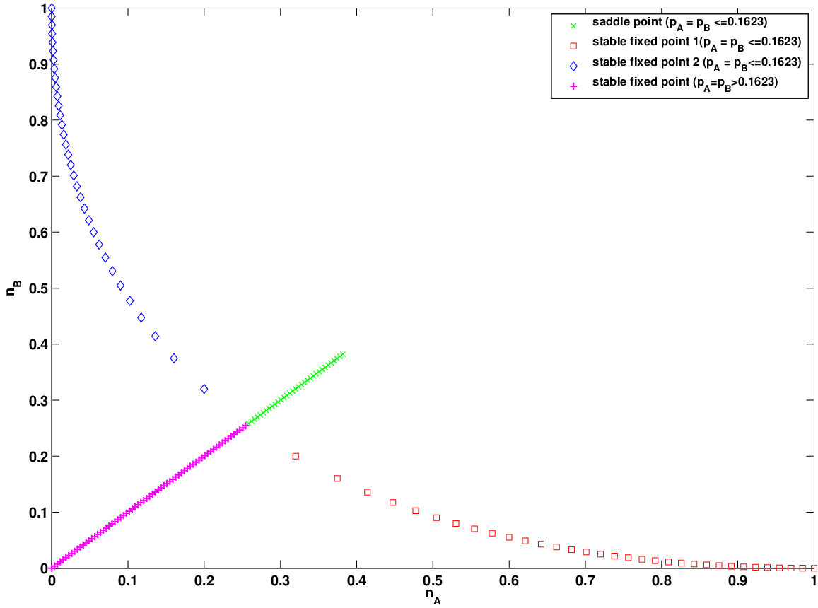
In order to study the nature of the transitions that occur when we cross the boundaries of the beak, we parametrize the system by denoting $p_{B}=cp_{A}$ where $c$ is a real number. Then, we systematically analyze the transitions occurring in two cases: (i) $c=1$ and (ii) $c\neq 1$. It can be shown that along the diagonal line $c=1$ the system undergoes a cusp bifurcation at $p_{A}=p_{B}=0.1623$. The movement of the fixed points as $p_{A}$ and $p_{B}$ are smoothly varied along the diagonal line is shown in Figure S1. Henceforth, we denote the value of $p_{A}$ and $p_{B}$ at the cusp as $p_{c}$. As is well known, at the cusp bifurcation two branches of a saddle-node (or fold) bifurcation meet tangentially [1]. These two bifurcation curves form the boundary of the beak shown in Fig. 1. A detailed analysis demonstrating that $p_{A}=p_{B}=p_{c}$ constitutes a cusp bifurcation, as well as a semi- analytical derivation of the bifurcation curves is provided in the Supporting Text S1 (Sections: 1, 2, 3). The cusp bifurcation point is analogous to a second-order (or continuous) critical point seen in equilibrium systems, while bifurcation curves are analogous to spinodal transition lines.

Next, we study the stochastic evolution of opinions on finite-sized complete graphs through simulations. Here, we systematically vary $c$ from $1$ to $0$ to obtain the right bifurcation curve, and therefore by virtue of the $A\mbox{-}B$ symmetry in the system, also obtain the left bifurcation curve. In particular for a given value of $c$ we obtain the transition point by varying $p_{A}$ (with $p_{B}=cp_{A}$) and measuring the quantity:

$$m=(n_{B}-n_{A})/(1-p_{A}-p_{B})$$

(2)

which we utilize as an order parameter. The above order parameter is analogous to the “magnetization” in a spin system as it captures the degree of dominance of opinion $B$ over opinion $A$ and is conventionally used to characterize the nature of phase transitions exhibited by such a system.

Another quantity, the Binder cumulant, defined as

$$U_{N}=1-\bigg[\frac{\langle m^{4}\rangle}{3\langle m^{2}\rangle^{2}}\bigg]$$

(3)

for a system of size $N$, is commonly used to distinguish between different types of phase transitions [17]. The utility of the Binder cumulant comes from the markedly different signatures we expect it to produce along a spinodal trajectory (e.g. $c=0.5$) - one that passes through the spinodal line - and one along a trajectory that passes through the critical point (e.g., along the diagonal, $c=1$). This difference arises from the following distinction in the evolution of the distribution of $m$, $P(m)$, along these trajectories. Along a spinodal trajectory starting from a point where $p_{A}=p_{B}$, an initially symmetric (about $m=0$), bimodal $P(m)$ becomes asymmetric and unimodal upon crossing the spinodal line, with the single mode eventually becoming a delta function. In contrast, along the diagonal trajectory in parameter space, $P(m)$ is initially a double-delta distribution (for $p_{A}=p_{B}\ll p_{c}$), symmetric about $m=0$, and it smoothly transitions to a zero-centred gaussian distribution as the critical point is crossed. The definition of $U_{N}$ indicates that $U_{N}=2/3$ for a delta function distribution (also for a symmetric, double-delta distribution about $m=0$), while $U_{N}=0$ for a zero-centered Gaussian distribution, and thus readily yields the limiting $U_{N}$ values at both extremes of the spinodal and diagonal trajectory. As illustrated in Fig. 2, $U_{N}$ as a function of $p_{A}$ shows distinct behaviors for $c=1$ and $c=0.5$, indicating the existence of a second-order (or continuous) transition point at $p_{A}=p_{B}=p_{c}(N)$ (Fig. 2(e)) and first-order (or discontinuous) phase transition points (Fig. 2(f)) along off-diagonal trajectories [17], respectively. The second-order critical point $p_{c}(N)$ converges to the mean-field value, $p_{c}\approx 0.1623$, as $N$ becomes larger. The dip observed in $U_{N}$ along the off-diagonal trajectory serves as an excellent estimator of the location of the first-order (spinodal) transition for a finite network. Thus, to reiterate, for a finite network, the second-order transition point and the first-order transition (spinodal) lines are respective analogues of the cusp bifurcation point and the saddle-node bifurcation curves observed in the mean-field case.

The fluctuations of the quantity $m$ can also be used to identify a transition point, particularly for the case of the second-order transition. In particular, in formal analogy with methods employed in the study of equilibrium spin systems, the scaled variance:

$$X_{N}=N\langle(|m|-\langle|m|\rangle)^{2}\rangle$$

(4)

serves as an excellent estimate for the second-order transition point $p_{c}$ for a finite network. As shown in Fig. 2(c), $X_{N}$ peaks at a particular value of $p_{A}$, with the size of the peak growing with $N$ (and expected to diverge as $N\to\infty$). In the case of the spinodal transition, one studies fluctuations of $m$ ($X_{N}=N\langle(m-\langle m\rangle)^{2}\rangle$) restricted to the metastable state [22, 23] until the spinodal point (Fig. 2(d)) at which the metastable state disappears, and fluctuations of $m$ in the unique stable state beyond the spinodal point (Fig. 2(d)).

Figure 3 shows the bifurcation (spinodal) lines obtained via simulations of finite complete graphs by using the Binder cumulant (Fig. 2(f))to identify the location of the spinodal phase transition, and demonstrates that its agreement with the mean-field curves improves as $N$ grows. The cusp points shown here are identified in simulations as the locations where $X_{N}$ reaches its peak value (Fig. 2(c)).

In the region within the beak, the switching time between the co-existing steady-states represents the longest time-scale of relevance in the system. The switching time is defined as the time the system takes to escape to a distinct co-existing steady-state, after having been trapped in one of the steady-states (see Fig. 4(a)). In stochastic systems exhibiting multistability or metastability, it is well known that switching times increase exponentially with $N$ for large $N$ (the weak-noise limit) [6, 25, 26, 4] Furthermore, the exponential growth rate of the switching time in such cases can be determined using the eikonal approximation [4, 27]. The basic idea in the approximation involves (i) assuming an eikonal form for the probability of occupying a state far from the steady-state and (ii) smoothness of transition probabilities in the master equation of the system. This allows the interpretation of fluctuational trajectories as paths conforming to an auxilliary Hamilton-Jacobi system. This in turn enables us to calculate the probability of escape allowing an optimal fluctuational path that takes the system from the vicinity of the steady-state to the vicinity of the saddle point of the deterministic system. The switching time is simply the inverse of the probability of escape along this optimal fluctuational path. We defer details of this procedure to Supporting text S1: Section 4. Using this approach we find that for the symmetric case, $p_{A}=p_{B}=p<p_{c}$, the exponential growth rate of the switching time $s\sim(p_{c}-p)^{\nu}$ with $\nu\approx 1.3$ (Fig. 4 (c) ). Thus, along the portion of the diagonal within the beak:

$$T_{\rm switching}\sim\exp[(p_{c}-p)^{\nu}N]$$

(5)

Outside the beak, the time to get arbitrarily close to the sole steady-state value grows logarithmically with $N$ (not shown).

The results presented so far show that there exists a transition in the time needed by a committed minority to influence the entire population to adopt its opinion, even in the presence of a committed opposition (i.e. in the case where both $p_{A},p_{B}>0$), as long as $p_{A},p_{B}<p_{c}$. (Note that the case $p_{A}>0,p_{B}=0$ was considered in [9]). For example, assume that initially all the uncommitted nodes adopt opinion $B$, and that $p_{A}=p_{B}<p_{c}$. Then, the steady-state that the system reaches in $\ln(N)$ time is the one in which the majority of nodes hold opinion $B$. Despite the fact that there exist committed agents in state $A$ continuously proselytizing their state, it takes an exponentially long time before a large (spontaneous) fluctuation switches the system to the $A$-dominant steady-state. For identical initial conditions, the picture is qualitatively the same if we increase $p_{A}$ keeping $p_{B}$ fixed, as long as $(p_{A},p_{B})$ lies within the beak. However, when $(p_{A},p_{B})$ lies on the bifurcation curve or beyond, the $B$-dominant steady-state vanishes, and with the same initial conditions - where $B$ is the initial majority - it takes the system only $\ln(N)$ time to reach the $A$-dominant state (the only existing steady-state). Thus, for every value of an existing committed fraction $p_{B}$ ($<p_{c}$) of $B$ nodes, there exists a corresponding critical fraction of $A$ nodes beyond which it is guaranteed that the system will reach an $A$ dominant state in $\ln(N)$ time, irrespective of the initial conditions. However, for any trajectory in the parameter space in a region where either $p_{A}$ or $p_{B}$ is (or both are) greater than $p_{c}$, no abrupt changes in dominance or consensus times are observed. Instead, the dominance of $A$ or $B$ at the single fixed point smoothly varies as the associated committed fractions are varied. Moreover, the system always reaches this single fixed point in $\ln(N)$ time.

Finally, we study how opinions evolve in the presence of committed groups on sparse graphs, most relevant to social networks. We study Erdős-Rényi (ER) random graphs [28] as well as Barabási-Albert networks [29]. For each of these sparse networks, we find the same qualitative behavior as found for the complete graph. As shown in Figs. 5, 6, as the average degree of the sparse networks increases, the bifurcation lines in parameter space tend to approach their mean-field counterparts. Although we do not study sparse networks analytically here, we note that in another instance of a phase transition for a similar model studied in [7], it was demonstrated using heterogeneous mean-field equations that the behavior of sparse networks is qualitatively similar to that of complete graphs. Figure 7 visually depicts typical instances of the evolution of opinions on an ER random graph for $(p_{A},p_{B})$ values within and outside the beak.

Using a simple model, we have explored and quantified possible outcomes for the evolution of opinions on a social network in the presence of groups committed to competing opinions. Broadly speaking, our results indicate that as long as the fraction, $p_{B}$, of nodes committed to a given opinion $B$ is held fixed at a value less than a critical value $p_{c}$, it is possible to induce the network to quickly tip over to a state where it widely adopts a competing opinion $A$, by introducing a fraction of nodes committed to opinion $A$. The value of the competing committed fraction, $p_{A}$, at which this tipping point arises depends on the value of $p_{B}$, and is determined by the bifurcation curve (see Fig. 1). Importantly, for a given value of $p_{B}<p_{c}$, the excess commitment $p_{A}-p_{B}$ required for the network to tip over to $A$ is a decreasing function of $p_{B}$ that reaches zero when $p_{B}=p_{c}$. While the critical value $p_{c}$ itself may depend on the network structure and its size, the feature described above holds for the three different classes of networks studied here. A corollary to this feature is that if the committed fraction $p_{B}$ is held fixed at a value greater than pc, increasing the competing committed fraction $p_{A}$ only yields continuous incremental gains in the adoption of A (i.e., no tipping point or discontinuous changes in opinions exist). We analytically determine that $p_{c}=0.1623$ for infinite-sized complete graphs, which as observed from our simulation results in Figs. 5, 6 appears to constitute a good upper bound to the value of $p_{c}$ for sparse networks.

Our results could be of utility in situations where public opinion is deadlocked due to the influence of competing committed groups. Perhaps one example of such a situation is the observed lack of consensus in the U.S. on the existence of human-induced climate change. Indeed, there is evidence in this particular case that the commitment of individuals to particular political ideologies may have an effect on their opinions [30].

Another scenario to which our model could bear some relevance is the adoption of competing industrial standards. Particularly in situations where a network of entities collaborate or are interdependent, there is a natural attempt at agreement in standards or protocols between interacting members. A classic example of this scenario is the case of the Sellers’ screw manufacturing standard that proliferated despite competition from the Whitworth standard [31]. A key factor responsible for the eventual success of the Sellers standard was William Sellers’ leveraging of his connections to corporations and manufacturers [32], whom he persuaded to become adopters of his standard . Furthermore, the network of interdependencies between industries at the dawn of the mass-manufacturing era played an important role in the adoption of the standard becoming widespread. It should be pointed out that in this case, the uncommitted members of the population initially adhered to neither standard - this situation can however be accommodated in our model by assigning each uncommitted his own unique “opinion” to begin with in close analogy to initial conditions for the original Naming Game [4, 5].

A more recent example of such a scenario is the competition between Flash and HTML5 in web-development. There is speculation that Flash, which until recently was the predominant platform for animated web content, is gradually ceding its dominance to HTML5 as a result of the increasing market-share of Apple’s mobile devices which exclusively support the latter [33].

A potential competition between DC fast charging standards is also expected as electric vehicles become increasingly popular with consumers. The front-runners in the mass manufacture of electric vehicles have opted for the CHAdeMO standard, and charging stations compatible with the standard have begun proliferating in the US, Europe and Japan [34, 35]. An alternative to CHAdeMO currently being developed by the Society for Automotive Engineers (SAE), which governs the development of standards in the US automotive industry, is being touted by some car manufacturers as more cost effective as well as technologically superior. However, by the time the first cars employing the SAE standard hit the market, CHAdeMO charging stations are expected to be rather widespread, thus making a competition between the two inevitable [36, 34]. As new collaborations are forged between car-makers especially in the area of electric vehicle development [37, 38] (in addition to collaborations with energy suppliers), the outcome of this competition could be significantly influenced by manufacturers who are already committed to one of the two standards through their investment in them.

To conclude, we have presented results from a simple, abstract model for understanding how opinions on a social network evolve through social influence when there are multiple groups within the network dedicated to competing opinions. Despite the simplicity of our model, we believe the insights provided here form a useful theoretical complement to data-driven studies [39] and randomized evaluations [40] aimed at understanding the spread of opinions.

Note: Subsequent to this paper’s initial posting on arxiv.org on 12/31/2011 and its acceptance for publication with minor revisions on 1/26/2012, S. Jolad sent us independent unpublished results by D. Linford, P. Hochendoner, A. Reagan, and S. Jolad addressing competing committed groups on the complete graph.

For notational simplicity we replace $n_{A}$ by $x$ and $n_{B}$ by $y$. The mean field equations describing the system with $p_{A}=p_{B}=p$, $0<p\leq 0.5$ then are:

	$\displaystyle\frac{dx}{dt}$	$\displaystyle=$	$\displaystyle-xy+(1-x-y-2p)^{2}+x(1-x-y-2p)+\frac{3}{2}p(1-x-y-2p)-px$
	$\displaystyle\frac{dx}{dt}$	$\displaystyle=$	$\displaystyle-xy+(1-x-y-2p)^{2}+y(1-x-y-2p)+\frac{3}{2}p(1-x-y-2p)-py$

where $n_{AB}=1-x-y-2p$. In the steady state, $dx/dt=dy/dt=0$, and the resulting equations can be solved to yield four solutions for $(x,y)$. Out of these one solution lies outside the valid range for all feasible values of $p$, i.e., $0<p\leq 0.5$. The valid fixed points for Eqs.  are:

	$\displaystyle x_{1}=\frac{3}{2}-\frac{1}{2}\sqrt{5-2p}-p$
	$\displaystyle y_{1}=\frac{3}{2}-\frac{1}{2}\sqrt{5-2p}-p$

	$\displaystyle x_{2}=\frac{1}{2}+\frac{1}{2}\sqrt{1-p^{2}-6p}-\frac{3}{2}p$
	$\displaystyle y_{2}=\frac{1}{2}-\frac{1}{2}\sqrt{1-p^{2}-6p}-\frac{3}{2}p$

	$\displaystyle x_{3}=\frac{1}{2}-\frac{1}{2}\sqrt{1-p^{2}-6p}-\frac{3}{2}p$
	$\displaystyle y_{3}=\frac{1}{2}+\frac{1}{2}\sqrt{1-p^{2}-6p}-\frac{3}{2}p$

Since the solutions are symmetric in $x$ and $y$, in order to investigate the range of $p$ over which these solutions are valid, we restrict our analysis to $y$. The solution $y_{1}$ is valid for all values of $p$. For $y_{2},y_{3}$ to be valid solutions, we require $U(p)=1-p^{2}-6p\geq 0$. $U(p)$ is a monotonically decreasing function for $p>0$, and the value of $p$ at which $U(p)$ first crosses zero is the critical point.

$$p_{c}=\sqrt{10}-3\approxeq 0.1623.$$

(2)

Thus, there exist three fixed points in the range $[0,p_{c}]$. In the range $(p_{c},0.5]$ only one valid fixed point exists, viz. $(x_{1},y_{1})$.

We can further examine the stability of the obtained fixed points. Linear stability analysis yields the following stability matrix:

$$Q=\left[\begin{array}[]{cc}-1-\frac{p}{2}&-2+2y^{*}+\frac{5}{2}p\\ -2+2x^{*}+\frac{5}{2}p&-1-\frac{p}{2}\\ \end{array}\right]$$

(3)

where $(x^{*},y^{*})$ is the fixed point under consideration.

The eigenvalues of the stability matrix at the fixed point are given by :

$$\lambda=-(2+p)\pm\sqrt{26p^{2}+(20(x^{*}+y^{*})-36)+16(1-x^{*}-y^{*}+x^{*}y^{*})},$$

and examination of the real part of these eigenvalues indicates that $(x_{2},y_{2})$ and $(x_{3},y_{3})$ are stable fixed points, and $(x_{1},y_{1})$ is an unstable fixed point (saddle point) for $p\leq p_{c}=0.1623$. For $p>p_{c}$, $(x_{1},y_{1})$, the only valid fixed point, is a stable fixed point. Supporting Figure 1 shows the movement of the fixed points in the phase space as a function of $p$.

Suppose that a one-dimensional parameter($\alpha$) dependent system

$$\frac{dx}{dt}=f(x;\alpha),x\in\Re^{1},\alpha\in\Re^{m}$$

(4)

with smooth function $f$, has an equilibrium at $x=0$ for $\alpha=0$, and let $f_{x}(0;0)=0$ and $f_{xx}(0;0)=0$ hold. Further, assume that the non-degeneracy conditions (e.g., $f_{xxx}(0;0)\neq 0$) are satisfied. Then the system undergoes a cusp bifurcation at $x=0$ [1].

We prove that such a cusp bifurcation is encountered in our system (i.e., Eq. ) at $p_{A}=p_{B}=p_{c}$ as we move along the diagonal in parameter space ($p_{A}=p_{B}$). Note that our system is two-dimensional. To be able to use the above theory, we first need to reduce the dimensionality of our system. The Center Manifold Theorem [2] guarantees the existence of a one-dimensional center manifold to which we can restrict our system, and such a system preserves the same behavior as the original system in the vicinity of the steady-state under consideration. Once we get the restricted system, we can perform the usual bifurcation analysis in one-dimensional system. Following this idea, we first shift the coordinates such that the origin is located at the critical point we found from the $p_{B}=p_{A}$ case (for simplicity, we denote $p_{A}$ by $p$ and $p_{B}$ by $r$), i.e., $(x_{0},y_{0};p_{0},r_{0})=(0.2565,0.2565;\sqrt{10}-3,\sqrt{10}-3)$. In the shifted coordinates, the eigenvalues and eigenvectors are given by $\Lambda=[0;-2.1623]$ and $V=[-0.7071,0.7071;0.7071,0.7071]$. Using the transformation $[\tilde{x}\;\tilde{y}]^{T}=V[x\;y]^{T}$, and after some algebraic manipulations, we obtain in the new co-ordinate system:

	$\displaystyle\frac{d\tilde{x}}{dt}$	$\displaystyle=$	$\displaystyle 0.7071(1.5p+0.2434)(p+r+1.414\tilde{y}-0.1623)$
			$\displaystyle-0.7071(1.5r+0.2434)(p+r+1.414\tilde{y}-0.1623)$
			$\displaystyle-0.7071(0.7071\tilde{x}+0.7071\tilde{y}+0.2566)(p+r+1.414\tilde{y}-0.1623)$
			$\displaystyle-0.7071(p+0.1623)(0.7071\tilde{x}+0.7071\tilde{y}+0.2566)$
			$\displaystyle+0.7071(0.7071\tilde{y}-0.7071\tilde{x}+0.2566)(p+r+1.414\tilde{y}-0.1623)$
			$\displaystyle+0.7071(r+0.1623)(0.7071\tilde{y}-0.7071\tilde{x}+0.2566)$
	$\displaystyle\frac{d\tilde{y}}{dt}$	$\displaystyle=$	$\displaystyle-0.7071(1.5r+0.2434)(p+r+1.414\tilde{y}-0.1623)$		(5)
			$\displaystyle-0.7071(1.5p+0.2434)(p+r+1.414\tilde{y}-0.1623)$
			$\displaystyle-0.7071(0.7071\tilde{x}+0.7071\tilde{y}+0.2566)(p+r+1.414\tilde{y}-0.1623)$
			$\displaystyle-0.7071(p+0.1623)(0.7071\tilde{x}+0.7071\tilde{y}+0.2566)$
			$\displaystyle-0.7071(0.7071\tilde{y}-0.7071\tilde{x}+0.2566)(p+r+1.414\tilde{y}-0.1623)$
			$\displaystyle-1.414(0.7071\tilde{x}+0.7071\tilde{y}+0.2566)(0.7071\tilde{y}-0.7071\tilde{x}+0.2566)$
			$\displaystyle-0.7071(r+0.1623)(0.7071\tilde{y}-0.7071\tilde{x}+0.2566)$
			$\displaystyle+1.414(p+r+1.414\tilde{y}-0.1623)^{2}$

Next, we use a quadratic approximation for the center manifold of the above system [2] i.e. we assume $\tilde{y}=h(\tilde{x})=\frac{1}{2}w\tilde{x}^{2}$. We can find $w$ by comparing two expressions obtained for $\frac{d\tilde{y}}{dt}$; the first is obtained by using $\frac{d\tilde{y}}{dt}=\frac{d\tilde{y}}{d\tilde{x}}\frac{d\tilde{x}}{dt}$ and then using the first equation in Eq. 5 and the quadratic approximation for $\tilde{y}$; the second is obtained by direct substitution of the quadratic approximation into the second equation in Eq. 5. Doing this yields:

$$\tilde{y}=h(\tilde{x})=-0.7071\tilde{x}^{2}/(4p+4r-2.1620)$$

Hence we obtain the following one dimensional system restricted to the one-dimensional center manifold:

	$\displaystyle\frac{\partial\tilde{x}}{\partial t}$	$\displaystyle=$	$\displaystyle 0.1814r-0.1814p-\tilde{x}(1.5p+1.5r)$		(6)
			$\displaystyle+0.7071(1.5p+0.2434)(p+r-0.1623)$
			$\displaystyle-0.7071(1.5r+0.2434)(p+r-0.1623)$
			$\displaystyle-\tilde{x}^{2}(0.7071(1.5p+0.2434)/(4p+4r-2.1623)$
			$\displaystyle-0.7071(1.5r+0.2434)/(4p+4r-2.1623)$
			$\displaystyle-0.7071(p+0.1623)/(8p+8r-4.3246)$
			$\displaystyle+0.7071(r+0.1623)/(8p+8r-4.3246))$
			$\displaystyle+\tilde{x}^{3}/(4p+4r-2.1623)$

It is easy to check that the origin in this transformed system satisfies the necessary conditions for a cusp bifurcation. The origin of this transformed system corresponds to the point $p_{A}=p_{B}=p_{c}$ in our original system Eq. . Thus, the system undergoes a cusp bifurcation at $p_{A}=p_{B}=p_{c}$ where $p_{c}=\sqrt{10}-3\approx 0.1623$.

In order to map out the first-order transition line (bifurcation curve) we adopt a semi-analytical approach. We assume $p_{B}=cp_{A}$ with $c<1$ to obtain the lower bifurcation curve (symmetry of the system allows us to obtain the upper bifurcation curve, given the lower one). Using Eqs. , the fixed point condition becomes (for simplicity, we denote $p_{A}$ by $p$):

	$\displaystyle f(x,y,p)$	$\displaystyle\equiv$	$\displaystyle-xy+(1-x-y-(1+c)p)^{2}+x(1-x-y-(1+c)p)$
		$\displaystyle+$	$\displaystyle\frac{3}{2}p(1-x-y-(1+c)p)-cpx=0$
	$\displaystyle g(x,y,p)$	$\displaystyle\equiv$	$\displaystyle-xy+(1-x-y-(1+c)p)^{2}+y(1-x-y-(1+c)p)$
		$\displaystyle+$	$\displaystyle\frac{3}{2}cp(1-x-y-(1+c)p)-py=0$

In addition, for a fold bifurcation, we also require that the stability matrix has an eigenvalue with zero real part. Since, the valid solutions in our case are always real, this is equivalent to requiring the determinant of the stability matrix to be zero. Thus the condition $|Q|=0$ (with $Q$ given by Eq. 3) along with Eqs.   enable us to determine for a given $c$, the location $(p_{A},cp_{A})$ at which the bifurcation occurs. By numerically solving these equations for different values of $c$, $0<c\leq 1$ at intervals of $0.1$, we obtain the lower bifurcation curve shown in Fig. 2 of the main text.

The master equation for our system takes the general form:

$$\frac{\partial P({\bf X},t)}{\partial t}=\sum_{{\bf r}}\bigg[W({\bf X}-{\bf r},{\bf r})P({\bf X}-{\bf r},t)-W({\bf X},{\bf r})P({\bf X},t)\bigg]$$

where ${\bf X}=[N_{A}\;N_{B}]^{T}$ denotes the (macro) state of the system as vector whose elements are the numbers of uncommitted nodes in state $A$ and $B$ respectively, $W({\bf X},{\bf r})$ is the probability of the transition from ${\bf X}$ to ${\bf X}+{\bf r}$, and ${\bf r}$ runs over the allowed set of displacement vectors in the space of macro-states. For our system, ${\bf r}$ runs over $[1\;0]^{T},[0\;1]^{T},[2\;0]^{T},[0\;2]^{T},[-1\;0]^{T},[0\;-1]^{T}$. The deterministic equations can be derived from this master equation and yield:

$$\frac{d{\bf X}_{\rm det}}{dt}=\sum_{\bf r}{\bf r}W({\bf X}_{\rm det},{\bf r})$$

The Wentzell-Friedlin theory [5, 6] assumes that for any path $[{\bf X}]$ in configuration space:

$$\mathcal{P}([{\bf X}])\sim\exp(-\mathcal{S}([{\bf X}]))$$

with $\mathcal{S}([{\bf X}^{*}])=0$ for the deterministic path $[{\bf X^{*}}]$. It follows that the dominant contribution to the probability of a fluctuation that brings the system to state ${\bf X}$ starting from a stable state ${\bf X}_{m}$ can be written as:

$$\mathcal{P}({\bf X}|{\bf X}_{m},t=0)=\exp(-S({\bf X}))$$

(7)

where

$$S({\bf X})=min_{[\bf{X}]:{\bf X}_{m}\rightarrow{\bf X}}\mathcal{S}([{\bf x}])$$

(8)

where the minimization is over all paths $[{\bf X}]$ starting at ${\bf X}_{m}$ and ending at ${\bf X}$. For ${\bf X}$ far away from the steady state, the probability of occupation $P(\bf{X})$ is equivalent to logarithmic accuracy to the probability of the most likely fluctuation, $\mathcal{P}({\bf X}|{\bf X}_{m},t=0)$ that brings the system to ${\bf X}$. The assumption of the form given by Eq. 7 for the occupation probability is known as the eikonal approximation.

Using a smoothness assumption for $W({\bf X},{\bf r})$, and since the changes in numbers of $A$ and $B$ nodes are $O(1)$, we can neglect the difference between $W({\bf X}-{\bf r},{\bf r})$ and $W({\bf X},{\bf r})$. With this approximation, the eikonal form for the occupation probabilities in the master equation yields the following equation for $S({\bf X})$ [4]:

$$H\bigg({\bf x},\frac{\partial s}{\partial{\bf x}}\bigg)=0$$

(9)

where

$$H({\bf x},{\bf p})=\sum_{\bf r}w({\bf x},{\bf r})(\exp({\bf r}{\bf p})-1)$$

(10)

and

$${\bf x}={\bf X}/N,\;\;w({\bf x},{\bf r})=W({\bf X},{\bf r})/N,\;\;s({\bf x})=S({\bf X})/N.$$

Eq. 9, is analogous to a Hamilton-Jacobi equation for the action of a system with Hamiltonian given by Eq. 10. The corresponding Hamilton equations of motion for components of position ${\bf x}$ and momentum ${\bf p}$ are:

$$\dot{x_{i}}=\frac{\partial H}{\partial p_{i}}\;\;\;\dot{p_{i}}=-\frac{\partial H}{x_{i}}$$

(11)

with $s({\bf x})$ playing the role of the classical action:

$$s([{\bf x}])=\int_{[{\bf x}]}L({\bf x},{\bf p})d{\bf x}=\int_{[{\bf x}]}{\bf p}\dot{{\bf x}}d{\bf x}$$

where $[{\bf x}]$ denotes a particular path obeying the equations of motion (Eqs. 11).

Following this Hamiltonian formulation to characterize the fluctuational paths of the system, our goal is to find the path with minimum action that reaches the separatrix in phase space of the deterministic motion, starting from the vicinity of the stable state under consideration [6, 4]. Arguments in [3] show that the fluctuational path reaching the separatrix with the minimal value of the action, is the path that passes through the saddle point. This is the optimal escape path, i.e., the path whose probability of occurrence dominates the probability of escape and we denote it by $[{\bf x}_{\rm opt}]$. This path can be found by integrating the equations of motion Eq. 11, and finding the required path that starts from the vicinity ${\bf x}_{m}$ to the saddle point ${\bf x}_{\rm saddle}$. Thus following Eqs. 7, 8 we have for the probability of escape from the current stable point in which the system is trapped:

$$P_{\rm escape}=P({\bf x}_{\rm saddle})\sim\exp[-Ns({\bf x}_{\rm saddle})]$$

(12)

where

$$s({\bf x}_{\rm saddle})=\int_{[{\bf x}_{\rm opt}]}L({\bf x},{\bf p})d{\bf x}$$

and the transition time (or time to escape from the steady state) follows:

$$T_{\rm switching}\sim\exp[Ns({\bf x}_{\rm saddle})]$$

(13)

In practice we start from some point ${\bf x}$ in the vicinity of the stable state, and to obtain the corresponding momenta ${\bf p}$ and action $s({\bf x})$, we employ a Gaussian approximation [4]:

$$S({\bf x})=\sum Z_{ij}(x_{i}-x_{i}^{m})(x_{j}-x_{j}^{m})$$

where $Z$ satisfies an algebraic Ricatti equation:

$${\bf Q}{\bf Z}^{-1}+{\bf Z}^{-1}{\bf Q}^{T}+{\bf K}=0$$

where $Q$ is the linear stability matrix (Eq. 3) evaluated at ${\bf x}_{m}$ and $K_{ij}=\sum_{\bf r}w({\bf x}_{m},{\bf r})r_{i}r_{j}$. Solving this Ricatti equation yields $Z$ which in turn yields $S({\bf x})$ and $p({\bf x})$.

In order to find the optimal fluctuational path of escape from a given steady state, we numerically generate fluctuational paths from various points close to the steady state (we explore points at intervals of $10^{-5}$ along the $x_{1}$ dimension and $10^{-2}$ along the $x_{2}$ dimension around the steady state) and find one that passes close enough (no greater than a distance of $10^{-5}$) to the saddle point. The equations of motion, Eqs. 11, are integrated using a trapezoidal rule to generate these paths starting with initial conditions obtained using the Gaussian approximation described above and subsequent numerical solution of the Ricatti equation (we use a Matlab Ricatti equation solver for the latter). The scaling behavior of switching times obtained using this approach for various committed fraction values as a function of distance from second-order transition (or cusp) point are shown in Fig. 5 of the main text.

References

- 1. Tarde G (1969) On Communication and Social Influence: Selected Papers. University of Chicago Press.
- 2. Lehmann J, Gonçalves B, Ramasco JJ, Cattuto C (2011) Dynamical classes of collective attention in twitter. CoRR abs/1111.1896.
- 3. Morris N (2000) Bridging the gap: An examination of diffusion and participatory approaches in development communication. Technical report, The CHANGE Project/The Manoff Group, Inc.
- 4. Steels L (1995) A self-organizing spatial vocabulary. Artificial Life 2: 319.
- 5. Baronchelli A, Felici M, Caglioti E, Loreto V, Steels L (2006) Sharp transition towards shared vocabularies in multi-agent systems. J Stat Mech:Theory Exp P06014: 0509075.
- 6. Dall’Asta L, Baronchelli A, Barrat A, Loreto V (2006) Nonequilibrium dynamics of language games on complex networks. Phys Rev E 74: 036105.
- 7. Baronchelli A, Dall’Asta L, Barrat A, Loreto V (2007) Nonequilibrium phase transition in negotiation dynamics. Phys Rev E 76: 051102.
- 8. Castelló X, Baronchelli A, Loreto V (2009) Consensus and ordering in language dynamics. Eur Phys J B 71: 557.
- 9. Xie J, Sreenivasan S, Korniss G, Zhang W, Lim C, et al. (2011) Social consensus through the influence of committed minorities. Phys Rev E 84: 011130.
- 10. Mobilia M (2003) Does a single zealot affect an infinite group of voters? Phys Rev Lett 91: 028701.
- 11. Galam S, Jacobs F (2007) The role of inflexible minorities in the breaking of democratic opinion dynamics. Physica A 381: 366 - 376.
- 12. Lu Q, Korniss G, Szymanski BK (2009) The naming game in social networks: community formation and consensus engineering. J Econ Interact Coord 4: 221.
- 13. Galam S (2010) Public debates driven by incomplete scientific data: The cases of evolution theory, global warming and h1n1 pandemic influenza. Physica A: Statistical Mechanics and its Applications 389: 3619 - 3631.
- 14. Mobilia M, Petersen A, Redner S (2007) On the role of zealotry in the voter model. J Stat Mech:Theory Exp 2007: P08029.
- 15. Biswas S, Sen P (2009) Model of binary opinion dynamics: Coarsening and effect of disorder. Phys Rev E 80: 027101.
- 16. Yildiz E, Acemoglu D, Ozdaglar AE, Saberi A, Scaglione A (2011) Discrete Opinion Dynamics with Stubborn Agents. SSRN eLibrary .
- 17. Landau DP, Binder K (2000) A Guide to Monte Carlo Simulations in Statistical Physics. Cambridge University Press, Cambridge, UK.
- 18. Mori T, Miyashita S, Rikvold PA (2010) Asymptotic forms and scaling properties of the relaxation time near threshold points in spinodal-type dynamical phase transitions. Phys Rev E 81: 011135.
- 19. Dykman MI, Mori E, Ross J, Hunt PM (1994) Large fluctuations and optimal paths in chemical kinetics. J Chem Phys 100: 5735-5750.
- 20. Gardner TS, Cantor CR, Collins JJ (2000) Construction of a genetic toggle switch in escherichia coli. Nature 403: 339–342.
- 21. Arnold VI (1988) Geometrical Methods in the Theory of Ordinary Differential Equations. Springer; 2nd edition.
- 22. Herrmann DW, Klein W, Stauffer D (1982) Spinodals in a long-range interaction system. Phys Rev Lett 49: 1262–1264.
- 23. Ray TS (1991) Evidence for spinodal singularities in high-dimensional nearest-neighbor ising models. Journal of Statistical Physics 62: 463-472.
- 24. Maier RS (1992) Large fluctuations in stochastically perturbed nonlinear systems: Applications in computing. In: Applications in computing, in 1992 Lectures on Complex Systems. Addison-Wesley.
- 25. Graham R, Tél T (1984-06-01) On the weak-noise limit of fokker-planck models. Journal of Statistical Physics 35: 729–748.
- 26. Gang H (1987) Stationary solution of master equations in the large-system-size limit. Phys Rev A 36: 5782–5790.
- 27. Luchinsky DG, McClintock PVE, Dykman MI (1998) Analogue studies of nonlinear systems. Rep Prog Phys 61: 889.
- 28. Bollobás B (2001) Modern Graph Theory. Cambridge University Press.
- 29. Barabási AL, Albert R (1999) Emergence of scaling in random networks. Science 286: 509-512.
- 30. Leiserowitz A, Maibach E, Roser-Renouf C, Hmielowski JD (2011) Politics and global warming: Democrats, republicans, independents, and the tea party. Yale University and George Mason University. New Haven, CT: Yale Project on Climate Change Communication.
- 31. Sinclair B (1969) At the turn of a screw: William sellers, the franklin institute, and a standard american thread. Technology and Culture 10.
- 32. Surowiecki J (2002). Turn of the century. Wired, 10.01.
- 33. Lee TB (2011). The death of flash and the quiet triumph of open standards. Forbes, http://onforb.es/quVd75.
- 34. Chambers N (2011). Power politics: Competing charging standards could threaten adoption of electric vehicles. Scientific American, http://bit.ly/mHDZ3j.
- 35. Blanco S (2011). Ecotality’s fast-charging units: Good news for leaf owners and (for now) nobody else. New York Times, Automobiles, http://nyti.ms/pQIdJC.
- 36. Csere C (2011). Electric-car makers’ quest: One plug to charge them all. New York Times, Automobiles, http://nyti.ms/oyLQsO.
- 37. Takahashi Y, Maxwell K (2011). B m w, toyota in partnership. Wall Street Journal, http://on.wsj.com/tsABDe.
- 38. Bunkley N (2011). Ford and toyota to work together on hybrid system for trucks. New York Times, Business Day, http://nyti.ms/nCALXh.
- 39. Madan A, Farrahi K, Gatica-Perez D, Pentland A (2011) Pervasive sensing to model political opinions in face-to-face networks. In: Proceedings of the 9th international conference on Pervasive computing. Berlin, Heidelberg: Springer-Verlag, Pervasive’11, pp. 214–231.
- 40. Banerjee A, Chandrasekhar A, Duflo E, Jackson M (2011) The diffusion of microfinance. MIT working paper.
1 Analysis of steady states for : existence of a critical value .
For notational simplicity we replace by and by . The mean field equations describing the system with , then are:
where . In the steady state, , and the resulting equations can be solved to yield four solutions for . Out of these one solution lies outside the valid range for all feasible values of , i.e., . The valid fixed points for Eqs. are:
Since the solutions are symmetric in and , in order to investigate the range of over which these solutions are valid, we restrict our analysis to . The solution is valid for all values of . For to be valid solutions, we require . is a monotonically decreasing function for , and the value of at which first crosses zero is the critical point.
- 1. V. I. Arnold. Geometrical Methods in the Theory of Ordinary Differential Equations. Springer; 2nd edition, 1988.
- 2. J. Carr. Applications of Centre Manifold Theory. Springer; 1 edition, 1981.
- 3. M. I. Dykman and M. A. Krivoglaz. Theory of fluctuational transitions between stable states of a nonlinear oscillator. Soviet Journal of Experimental and Theoretical Physics, 50:30, July 1979.
- 4. M. I. Dykman, Eugenia Mori, John Ross, and P. M. Hunt. Large fluctuations and optimal paths in chemical kinetics. J. Chem. Phys., 100(8):5735–5750, 1994.
- 5. M. I. Freidlin and A. D. Wentzell. Random Perturbations of Dynamical Systems. Springer-Verlag, 1984.
- 6. Robert S. Maier. Large fluctuations in stochastically perturbed nonlinear systems: Applications in computing. In Applications in computing, in 1992 Lectures on Complex Systems. Addison-Wesley, 1992.