Two-Manifold Problems
Byron Boots Geoffrey J. Gordon
Machine Learning Department Carnegie Mellon University Pittsburgh, PA 15213 beb@cs.cmu.edu Machine Learning Department Carnegie Mellon University Pittsburgh, PA 15213 ggordon@cs.cmu.edu
Abstract
Recently, there has been much interest in spectral approaches to learning manifolds—so-called kernel eigenmap methods. These methods have had some successes, but their applicability is limited because they are not robust to noise. To address this limitation, we look at two-manifold problems, in which we simultaneously reconstruct two related manifolds, each representing a different view of the same data. By solving these interconnected learning problems together and allowing information to flow between them, two-manifold algorithms are able to succeed where a non-integrated approach would fail: each view allows us to suppress noise in the other, reducing bias in the same way that an instrumental variable allows us to remove bias in a linear dimensionality reduction problem. We propose a class of algorithms for two-manifold problems, based on spectral decomposition of cross-covariance operators in Hilbert space. Finally, we discuss situations where two-manifold problems are useful, and demonstrate that solving a two-manifold problem can aid in learning a nonlinear dynamical system from limited data.
1 Introduction
Manifold learning algorithms are non-linear methods for embedding a set of data points into a low-dimensional space while preserving local geometry. Recently, there has been a great deal of interest in spectral approaches to learning manifolds. These kernel eigenmap methods include Isomap [1], Locally Linear Embedding (LLE) [2], Laplacian Eigenmaps (LE) [3], Maximum Variance Unfolding (MVU) [4], and Maximum Entropy Unfolding (MEU) [5]. These approaches can be viewed as kernel principal component analysis [6] with specific choices of manifold kernels [7]: they seek a small set of latent variables that, through a nonlinear mapping, explains the observed high-dimensional data.
Despite the popularity of kernel eigenmap methods, they are limited in one important respect: they generally only perform well when there is little or no noise. Several authors have attacked this problem using methods including neighborhood smoothing [8] and robust principal components analysis [9, 10], with some success under limited noise. Unfortunately, the problem is fundamentally ill posed without some sort of side information about the true underlying signal: by design, manifold methods will recover extra latent dimensions which “explain” the noise.
We take a different approach to the problem of learning manifolds from noisy observations. We assume access to a set of instrumental variables: variables that are correlated with the true latent variables, but uncorrelated with the noise in observations. Such instrumental variables can be used to separate signal from noise, as described in Section 3. Instrumental variables have been used to allow consistent estimation of model parameters in many statistical learning problems, including linear regression [11], principal component analysis [12], and temporal difference learning [13]. Here we extend the scope of this technique to manifold learning. We will pay particular attention to the case of observations from two manifolds, each of which can serve as instruments for the other. We call such problems two-manifold problems.
In one-manifold problems, when the noise variance is significant compared to the manifold’s geometry, kernel eigenmap methods are biased: they will fail to recover the true manifold, even in the limit of infinite data. Two-manifold methods, by contrast, can succeed in this case: we propose algorithms based on spectral decompositions related to cross-covariance operators in a tensor product space of two different manifold kernels, and show that the instrumental variable idea suppresses noise in practice. We also examine some theoretical properties of two-manifold methods: we argue consistency for a special case in Sec. 3.2.3, but we leave a full theoretical analysis of these algorithms to future work.
The benefits of the spectral approach to two-manifold problems are significant: first, the spectral decomposition naturally solves the manifold alignment problem by finding low-dimensional manifolds (defined by the left and right eigenvectors) that explain both sets of observations. Second, the connection between manifolds and covariance operators opens the door to solving more-sophisticated machine learning problems with manifolds, including nonlinear analogs of canonical correlations analysis (CCA) and reduced-rank regression (RRR).
As an example of this last point, subspace identification approaches to learning non-linear dynamical systems depend critically on instrumental variables and the spectral decomposition of (potentially infinite-dimensional) covariance operators [14, 15, 16, 17, 18]. Two-manifold problems are a natural fit: by relating the spectral decomposition to our two-manifold method, subspace identification techniques can be forced to identify a manifold state space, and consequently, to learn a dynamical system that is both accurate and interpretable, outperforming the current state of the art.
2 Preliminaries
We begin by looking at two well-known classes of nonlinear dimensionality reduction: kernel principal component analysis (kernel PCA) and manifold learning.
2.1 Kernel PCA
Kernel PCA [6] is a generalization of principal component analysis [12]: we first map our -dimensional inputs to a higher-dimensional feature space using a feature mapping , and then find the principal components in this new space. If the features are sufficiently expressive, kernel PCA can find structure that regular PCA misses. However, if is high- or infinite-dimensional, the straightforward approach to PCA, via an eigendecomposition of a covariance matrix, is in general intractable. Kernel PCA overcomes this problem by assuming that is a reproducing-kernel Hilbert space (RKHS), and that the feature mapping is implicitly defined via an efficiently-computable kernel function . Popular kernels include the linear kernel (which identifies the feature space with the input space) and the RBF kernel .
Conceptually, if we define an infinitely-tall “matrix” with columns , , our goal is to recover the eigenvalues and eigenvectors of the centered covariance operator , where is the centering matrix . To avoid working with the high- or infinite-dimensional covariance operator, we instead define the Gram matrix . The nonzero eigenvalues of the centered covariance are the same as those of the centered Gram matrix . And, the corresponding unit-length eigenvectors of are given by , where and are the eigenvalues and eigenvectors of [6]. If data weights (a diagonal matrix) are present, we can instead decompose the weighted centered Gram matrix . (Note that, perhaps confusingly, we center first and multiply by the weights only after centering; the reason for this order will become clear below, in Section 2.2.)
2.2 Manifold Learning
Spectral algorithms for manifold learning, sometimes called kernel eigenmap methods, include Isomap [1], Locally Linear Embedding (LLE) [2], Laplacian Eigenmaps (LE) [3], and Maximum Variance Unfolding (MVU) [4]. These methods seek a nonlinear function that maps a high-dimensional set of data points to a lower-dimensional space while preserving the manifold on which the data lies. The main insight behind these methods is that large distances in input space are often meaningless due to the large-scale curvature of the manifold; so, ignoring these distances can lead to a significant improvement in dimensionality reduction by “unfolding” the manifold.
Interestingly, these algorithms can be viewed as special cases of kernel PCA where the Gram matrix is constructed over the finite domain of the training data in a particular way [7]. Specifically, kernel eigenmap methods first induce a neighborhood structure on the data, capturing a notion of local geometry via a graph, where nodes are data points and edges are neighborhood relations. Then they solve an eigenvalue or related problem based on the graph to embed the data into a lower dimensional space while preserving the local relationships. Here we just describe LE; the other methods have a similar intuition, although the details and performance characteristics differ.
In LE, neighborhoods are summarized by an adjacency matrix , computed by nearest neighbors: element is nonzero whenever the th point is one of the nearest neighbors of the th point, or vice versa. Non-zero weights are typically either set to 1 or computed according to a Gaussian RBF kernel: . Now let , and set . Finally, eigendecompose to get a low dimensional embedding of the data points, discarding the top eigenvector (which is trivial): if , the embedding is . To relate LE to kernel PCA, note that is already centered, i.e., . So, we can view LE as performing weighted kernel PCA, with Gram matrix and data weights .11 1 The original algorithm actually looks for the smallest eigenvalues of , which is equivalent. The matrix is the graph Laplacian for our neighborhood graph, and is the weighted graph Laplacian—hence the algorithm name “Laplacian eigenmaps.”,22 2 The centering step is vestigial: we can include it, , but it has no effect. The discarded eigenvector (which corresponds to eigenvalue 0 and to a constant coordinate in the embedding) similarly is vestigial: we can discard it or not, and it doesn’t affect pairwise distances among embedded points. Interestingly, previous papers on the connection between Laplacian eigenmaps and the other algorithms mentioned here seem to contain an imprecision: they typically connect dropping the top (trivial) eigenvector with the centering step—e.g., see [5]. ,33 3 A minor difference is that LE does not scale its embedding using the eigenvalues of ; the related diffusion maps algorithm [19] does.
The weighted Gram matrix can be related to a random walk on the graph defined by : if we add the identity and make a similarity transform (both operations that preserve the eigensystem), we get , a stochastic transition matrix for the walk. So, Laplacian eigenmaps can be viewed as trying to keep points close together when they are connected by many short paths in our graph.
3 Bias and Instrumental Variables
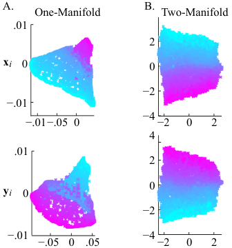
Kernel eigenmap methods are very good at dimensionality reduction when the original data points sample a high-dimensional manifold relatively densely, and when the noise in each sample is small compared to the local curvature of the manifold (or when we don’t care about recovering curvature on a scale smaller than the noise). In practice, however, observations are frequently noisy. Depending on the nature of the noise, manifold-learning algorithms applied to these datasets produce biased embeddings. See Figures 1–2, the “noisy swiss rolls,” for an example of how noise can bias manifold learning algorithms.
To see why, we examine PCA, a special case of manifold learning methods, and look at why it produces biased embeddings in the presence of noise. We first show how overcome this problem in the linear case, and then use these same ideas to fix kernel PCA, a nonlinear algorithm. Finally, in Sec. 4, we extend these ideas to fully general kernel eigenmap methods.
3.1 Bias in Finite-Dimensional Linear Models
Suppose that is a noisy view of some underlying low-dimensional latent variable : for a linear transformation and i.i.d. zero-mean noise term . Without loss of generality, we assume that and are centered, and that and both have full column rank: any component of in the nullspace of doesn’t affect .
In this case, PCA on will generally fail to recover : the expectation of is , while we need to be able to recover a transformation of or . The unwanted term will, in general, affect all eigenvalues and eigenvectors of , causing us to recover a biased answer even in the limit of infinite data.
3.1.1 Instrumental Variables
We can fix this problem for linear embeddings: instead of plain PCA, we can use what might be called two-subspace PCA. This method finds a statistically consistent solution through the use of an instrumental variable [11, 12], an observation that is correlated with the true latent variables, but uncorrelated with the noise in .
Importantly, picking an instrumental variable is not merely a statistical aid, but rather a value judgement about the nature of the latent variable and the noise in the observations. In particular, we are defining the noise to be that part of the variability which is uncorrelated with the instrumental variable, and the signal to be that part which is correlated.
In our example above, a good instrumental variable is a different (noisy) view of the same underlying low-dimensional latent variable: for some full-column-rank linear transformation and i.i.d. zero-mean noise term . The expectation of the empirical cross covariance is then : the noise terms, being independent and zero-mean, cancel out. (And the variance of each element of goes to 0 as .)
In this case, we can identify the embedding by computing the singular value decomposition (SVD) of the covariance: let , where and are orthonormal and is diagonal. To reduce noise, we can keep just the columns of , , and which correspond to the top largest singular values (diagonal entries of ): . If we set to be the true dimension of , then as , will converge to an orthonormal basis for the range of , and will converge to an orthonormal basis for the range of . The corresponding embeddings are then given by and .
Interestingly, we can equally well view as an instrumental variable for : we simultaneously find consistent embeddings of both and , using each to unbias the other.
3.1.2 Whitening: Reduced-Rank Regression and Cannonical Correlation Analysis
Going beyond two-subspace PCA, there are a number of interesting spectral decompositions of cross-covariance matrices that involve transforming the variables and before applying a singular value decomposition [12]. For example, in reduced-rank regression [20, 12], we want to estimate . Define and . Then the ordinary regression of on is , where the regularization term ensures that the matrix inverse is well-defined. For a reduced-rank regression, we instead project onto the set of rank- matrices: . In our example above, so long as we let as , will again converge to an orthonormal basis for the range of .
To connect back to two-subspace PCA, we can show that RRR is the same as two-subspace PCA if we first whiten . That is, we can equivalently define for RRR to be the top left singular vectors of the covariance between and the whitened instruments . (Here, stands for the symmetric square root of , which is guaranteed to exist and be invertible if is symmetric and positive definite.) Whitening means transforming a covariance matrix toward the identity: if and has full rank, then , while if is near 0, then .
For symmetry, we can whiten both and before computing their covariance. An SVD of the resulting doubly-whitened cross-covariance matrix is called canonical correlation analysis [21], and the resulting singular values are called canonical correlations.
3.2 Bias in Learning Nonlinear Models
We now extend the analysis of Section 3.1 to nonlinear models. We assume noisy observations , where is the desired low-dimensional latent variable, is an i.i.d. noise term, and is a smooth function with smooth inverse (so that lies on a manifold). Our goal is to recover and up to identifiability.
Kernel PCA (Sec. 2.1) is a common approach to this problem. In the realizable case, kernel PCA gets the right answer: that is, suppose that has dimension , and that we have at least independent samples. And, suppose that is a linear function of . Then, the Gram matrix or the covariance “matrix” will have rank , and we can reconstruct a basis for the range of from the top eigenvectors of the Gram matrix. (Similarly, if is near linear and the variance of is small, we can expect kernel PCA to work well, if not perfectly.)
However, just as PCA recovers a biased answer in the finite dimensional case when the variance of is nonzero, kernel PCA will also recover a biased answer in this case, even in the limit of infinite data. The bias of kernel PCA follows immediately from the example at the beginning of Section 3: if we use a linear kernel, kernel PCA will simply reproduce the bias of ordinary PCA.
3.2.1 Instrumental Variables
By analogy to two-subspace PCA, a a natural generalization of kernel PCA is two-subspace kernel PCA, which we can accomplish via a kernelized SVD of a cross-covariance operator in Hilbert space. Given a joint distribution over two variables on and on , with feature maps and (corresponding to kernels and ), the cross-covariance operator is . The cross-covariance operator reduces to an ordinary cross-covariance matrix in the finite-dimensional case; in the infinite-dimensional case, it can be viewed as a kernel mean map descriptor [22] for the joint distribution .
The concept of a cross-covariance operator is helpful because it allows us to extend the methods of instrumental variables to infinite dimensional RKHSs. In our example above, a good instrumental variable is a different (noisy) view of the same underlying low-dimensional latent variable: for some smoothly invertible function and i.i.d. zero-mean noise term .
We proceed now to derive the kernel SVD for a cross-covariance operator.44 4 The kernel SVD algorithm previously appeared as an intermediate step in [17, 23]; here we generalize the algorithm to weighted cross covariance operators in Hilbert space and give a more complete description, both because the method is interesting in its own right, and because this generalized SVD will serve as a step in our two-manifold algorithms. We show below (Sec. 3.2.3) that the kernel SVD of the cross-covariance operator leads to a consistent estimate of the shared latent variables in two-manifold problems which satisfy appropriate assumptions.
Conceptually, our inputs are “matrices” and whose columns are respectively and , along with data weights and . The centered empirical covariance operator is then . The goal of the kernel SVD is then to factor (or possibly the weighted variant ) so that we can recover the desired bases for and .
However, this conceptual algorithm is impractical, since can be high- or infinite-dimensional. Instead, we can perform an SVD on the covariance operator in Hilbert space via a trick analogous to kernel PCA. We first show how to perform an SVD on a covariance matrix using Gram matrices in finite-dimensional space, and then we extend the method to infinite dimensional spaces in Section 3.2.3.
3.2.2 SVD via Gram matrices
We start by looking at a Gram matrix formulation of finite dimensional SVD. In standard SVD, the singular values of are the square roots of the eigenvalues of (where ), and the left singular vectors are defined to be the corresponding eigenvectors. We can find identical eigenvectors and eigenvalues through centered Gram matrices and . Let be the right eigenvector of so that . Premultiplying by yields
and regrouping terms gives us where . So, is an eigenvalue of , is a singular value of , and is the corresponding unit length left singular vector. An analogous argument shows that, if is a unit-length right singular vector of , then , where is a unit-length left eigenvector of . Furthermore, we can easily incorporate weights into SVD by using weighted matrices and in place of and .
3.2.3 Two-subspace PCA in RKHSs
The machinery developed in Section 3.2.2 allows us to solve the two-subspace kernel PCA problem by computing the singular values of the weighted empirical covariance operator . We define and to be the Gram matrices whose elements are and respectively, and then compute the eigendecomposition of . This method avoids any computations in infinite-dimensional spaces; and, it gives us compact representations of the left and right singular vectors. E.g., if is a right eigenvector of , then the corresponding singular vector is , where is the weight assigned to data point .
Under appropriate assumptions, we can show that the SVD of the empirical cross-covariance operator converges to the desired value. Suppose that is a linear function of , and similarly, that is a linear function of .55 5 The assumption of linearity is restrictive, but appears necessary: in order to learn a representation of a manifold using factorization-based methods, we need to pick a kernel which flattens out the manifold into a subspace. This is why kernel eigenmap methods are generally more successful than plain kernel PCA: by learning an appropriate kernel, they are able to adapt their nonlinearity to the shape of the target manifold. The noise terms and are by definition zero-mean; and they are independent of each other, since the first depends only on and the second only on . So, the noise terms cancel out, and the expectation of is the true covariance . If we additionally assume that the noise terms have finite variance, the product-RKHS norm of the error vanishes as .
The remainder of the proof follows from the proof of Theorem 1 in [17] (the convergence of the empirical estimator of the kernel covariance operator). In particular, the top left singular vectors of converge to a basis for the range of (considered as a function of ); similarly, the top right singular vectors of converge to a basis for the range of .
3.2.4 Whitening and Kernel SVD
Just as one can use kernel SVD to solve the two-subspace kernel PCA problem for high- or infinite-dimensional feature space, one can also compute the kernel versions of CCA and RRR. (Kernel CCA is a well-known algorithm, though our formulation here is different than in [23], and kernel RRR is to our knowledge novel.) Again, these problems can be solved by pre-whitening the feature space before applying kernel SVD.
To compute a RRR from centered covariates in Hilbert space to centered responses in Hilbert space, we find the kernel SVD of the -whitened covariance matrix: first we define and ; next we compute ; and, finally, we perform kernel SVD by finding the singular value decomposition of .
Similarly, for CCA in Hilbert space, we find the kernel SVD of the - and -whitened covariance matrix: .
If data weights are present, we use instead weighted centered Gram matrices and . Then, to generalize RRR and CCA to RKHSs, we can compute the eigendecompositions of Equations 1a–b, respectively:
| (1a) | |||
| (1b) | |||
The consistency of both approaches follows directly from the consistency of kernel SVD, so long as we let as [24].
4 Two-Manifold Problems
Now that we have extended the instrumental variable idea to RKHSs, we can also expand the scope of manifold learning to two-manifold problems, where we want to simultaneously learn two manifolds for two covarying lists of observations, each corrupted by uncorrelated noise.66 6 The uncorrelated noise assumption is extremely mild: if some latent variable causes correlated changes in our measurements on the two manifolds, then we are making the definition that it is part of the desired signal to be recovered. No other definition seems reasonable: if there is no difference in statistical behavior between signal and noise, then it is impossible to use a statistical method to separate signal from noise. The idea is simple: we view manifold learners as constructing Gram matrices, then apply the RKHS instrumental variable idea of Sec. 3. As we will see below, this procedure allows us to regain good performance when observations are noisy.
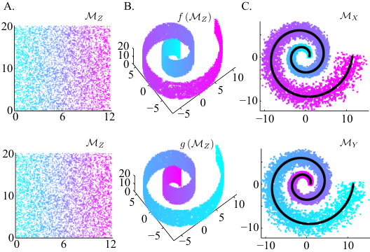
Suppose we are given two set of observations residing on (or near) two different manifolds: on a manifold and on a manifold . Further suppose that both and are noisy functions of a latent variable , itself residing on a latent -dimensional manifold : and . We assume that the functions and are smooth, so that and trace out submanifolds and . We further assume that the noise terms and move and within their respective manifolds and : this assumption is without loss of generality, since we can can always increase the dimension of the manifolds and to allow an arbitrary noise term. See Figure 1 for an example.
If the variance of the noise terms and is too high, or if and are higher-dimensional than the latent manifold (i.e., if the noise terms move and away from and ), then it may be difficult to reconstruct or separately from or . Our goal, therefore, is to use and together to reconstruct both manifolds simultaneously: the extra information from the correspondence between and will make up for noise, allowing success in the two-manifold problem where the individual one-manifold problems are intractable.
Given samples of i.i.d. pairs from two manifolds, we propose a two-step spectral learning algorithm for two-manifold problems: first, use either a given kernel or an ordinary one-manifold algorithm such as LE or LLE to compute weighted centered Gram matrices and from and separately. Second, use use one of the cross-covariance methods from Section 3.2.4, such as kernel SVD, to recover the embedding of points in . The procedure, called instrumental eigenmaps, is summarized in Algorithm 1.
In: i.i.d. pairs of observations
Out: embeddings and
For example, if we are using LE (Section 2.2), then and , where and are computed from , and and are computed from . We then perform a singular value decomposition and truncate to the top singular values:
The embeddings for and are then given by
Computing eigenvalues of instead of or alone will alter the eigensystem: it will promote directions within each individual learned manifold that are useful for predicting coordinates on the other learned manifold, and demote directions that are not useful. As shown in Figure 2, this effect strengthens our ability to recover relevant dimensions in the face of noise.
5 Two-Manifold Detailed Example: Learning Dynamical Systems
A longstanding goal in machine learning and robotics has been to learn accurate, economical models of dynamical systems directly from observations. This task requires two related subtasks: 1) learning a low dimensional state space, which is often known to lie on a manifold; and 2) learning the system dynamics. We propose tackling this problem by combining spectral learning algorithms for non-linear dynamical systems [14, 15, 16, 18, 25, 17] with two-manifold methods.
Any of the above-cited spectral learning algorithms can be combined with two-manifold methods. Here, we focus on one specific example: we show how to combine HSE-HMMs [17], a powerful nonparametric approach to modeling dynamical systems, with manifold learning. Specifically, we look at one important step in the HSE-HMM learning algorithm: the original approach uses kernel SVD to discover a low-dimensional state space, and we propose replacing the kernel SVD with a two-manifold method. We demonstrate that the resulting manifold HSE-HMM can outperform standard HSE-HMMs (and many other well-known methods for learning dynamical systems) on a difficult real-world example: the manifold HSE-HMM accurately discovers a curved low-dimensional manifold which contains the state space, while other methods discover only a (potentially much higher-dimensional) subspace which contains this manifold.
5.1 Hilbert Space Embeddings of HMMs
The key idea behind spectral learning of dynamical systems is that a good latent state is one that lets us predict the future. HSE-HMMs implement this idea by finding a low-dimensional embedding of the conditional probability distribution of sequences of future observations, and using the embedding coordinates as state. Song et al. [17] suggest finding this low-dimensional state space as a subspace of an infinite dimensional RKHS.
Intuitively, we might think that we could find the best state space by performing PCA or kernel PCA of sequences of future observations. That is, we would sample sequences of future observations from a dynamical system. (If our training data consists of a single long sequence of observations, we can collect our sample by picking random time steps . Each sample is then a sequence of observations starting at time .) We would then construct a Gram matrix , whose element is . Finally, we would find the eigendecomposition of the centered Gram matrix as in Section 2.1. The resulting embedding coordinates would be tuned to predict future observations well, and so could be viewed as a good state space.
However, the state space found by kernel PCA is biased: it typically includes noise, information that cannot be predicted from past observations. We would like instead to find a low dimensional state space that embeds the probability distribution of possible futures conditioned on the past. In particular, we want to find a state space that is uncorrelated with the noise in the future observations. From a two-manifold perspective, we view features of the past as instrumental variables to unbias the future.
Therefore, in addition to sampling sequences of future observations, we sample corresponding sequences of past observations : sequence ends at time . We then construct a Gram matrix , whose element is . From we construct the centered Gram matrix . Finally, we identify the state space using a kernel SVD as in Section 3.2.3: (there are no data weights for HSE-HMMs). The left singular “vectors” (reconstructed from as in Section 3.2.3) now identify a subspace in which the system evolves. From this subspace, we can proceed to identify the parameters of the dynamical system as in Song et al. [17].77 7 Other approaches such as CCA and RRR have also been successfully used for finite-dimensional spectral learning algorithms [18], suggesting that kernel SVD could be replaced by kernel CCA or kernel RRR (Section 3.2.4).
5.2 Manifold HSE-HMMs
In contrast with HSE-HMMs, we are interested in modeling a dynamical system whose state space lies on a low-dimensional manifold, even if this manifold is curved to occupy a higher-dimensional subspace (an example is given in Section 5.3, below). We want to use this additional knowledge to constrain the learning algorithm and produce a more accurate model for a given amount of training data.
To do so, we replace the kernel SVD by a two-manifold method. That is, we learn weighted centered Gram matrices and for the future and past observations, using a manifold method like LE or LLE (see Section 2.2). Then we apply a SVD to in order to recover the latent state space.
5.3 Slotcar: A Real-World Dynamical System

Here we look at the problem of tracking and predicting the position of a slotcar with attached inertial measurement unit (IMU) racing around a track. The setup consisted of a track and a miniature car (1:32 scale model) guided by a slot cut into the track. Figure 3(A) shows setup. At a rate of 10Hz, we extracted the estimated 3-D acceleration and angular velocity of the car. An overhead camera also supplied estimates of the 2-dimensional location of the car.
We collected 3000 successive observations while the slot car circled the track controlled by a constant policy (with varying speeds). The goal was to learn a dynamical model of the noisy IMU data, and, after filtering, to predict current and future 2-dimensional locations. We used the first 2000 data points as training data, and held out the last 500 data points for testing the learned models. We trained four models, and evaluated these models based on prediction accuracy, and, where appropriate, the learned latent state.
First, we trained a 20-dimensional embedded HMM with the spectral algorithm of Song et al. [17], using sequences of 150 consecutive observations. Following Song et al., we used Gaussian RBF kernels, setting the bandwidth parameter with the “median trick”, and using regularization parameter . Second, we trained a similar 20-dimensional embedded HMM with LE kernels. The number of nearest neighbors was selected to be 50, and the other parameters were set to be identical to the first model. (So, the only difference is that the first model performs a kernel SVD to find the subspace on which the dynamical system evolves, while the second model solves a two-manifold problem.) Third, for comparison’s sake, we trained a 20-dimensional Kalman filter using the N4SID algorithm [26] with Hankel matrices of 150 time steps; and finally, we learned a 20-state discrete HMM (with 400 levels of discretization for observations) using the EM algorithm.
Before investigating the predictive accuracy of the learned dynamical systems, we looked at the learned state space of the first three models. These models differ mainly in their kernel: Gaussian RBF, learned manifold from Laplacian Eigenmaps, or linear. As a test, we tried to reconstruct the 2-dimensional locations of the car from each of the three latent state spaces: the more accurate the learned state space, the better we expect to be able to reconstruct the locations. Results are shown in Figure 3(B); the learned manifold is the clear winner.
Finally we examined the prediction accuracy of each model. We performed filtering for different extents , then predicted the car location for a further steps in the future, for . The root mean squared error of this prediction in the 2-dimensional location space is plotted in Figure 3(C). The Manifold HMM learned by the method detailed in Section 5.2 consistently yields lower prediction error for the duration of the prediction horizon. This is important: not only does the manifold HSE-HMM provide a model that better visualizes the data that we want to predict, but it is significantly more accurate when filtering and predicting than classic and state-of-the-art alternatives.
6 Related Work
While preparing this manuscript, we learned of the simultaneous and independent work of Mahadevan et al. [27]. This paper defines one particular two-manifold algorithm, maximum covariance unfolding (MCU), by extending maximum variance unfolding; but, it does not discuss how to extend other one-manifold methods. It also does not discuss any asymptotic properties of the MCU method, such as consistency.
A similar problem to the two-manifold problem is manifold alignment [28, 29], which builds connections between two or more data sets by aligning their underlying manifolds. Generally, manifold alignment algorithms either first learn the manifolds separately and then attempt to align them based on their low-dimensional geometric properties, or they take the union of several manifolds and attempt to learn a latent space that preserves the geometry of all of them [29]. Our aim is different: we assume paired data, where manifold alignments do not; and, we focus on learning algorithms that simultaneously discover manifold structure (as kernel eigenmap methods do) and connections between manifolds (as provided by, e.g., a top-level learning problem defined between two manifolds).
This type of interconnected learning problem has been explored before in a different context via reduced-rank regression (RRR) [30, 31, 20] and sufficient dimension reduction (SDR) [32, 33, 34]. RRR is a linear regression method that attempts to estimate a set of coefficients to predict response vectors from covariate vectors under the constraint that is low rank (and can therefore be factored). In SDR, the goal is to find a linear subspace of covariates that makes response vectors conditionally independent of the s. The formulation is in terms of conditional independence, and, unlike in RRR, no assumption is made on the form of the regression from to . Unfortunately, SDR pays a price for the relaxation of the linear assumption: the solution to SDR problems usually requires a difficult non-linear non-convex optimization.
Manifold kernel dimension reduction [35], finds an embedding of covariates using a kernel eigenmap method, and then attempts to find a linear transformation of some of the dimensions of the embedded points to predict response variables . The response variables are constrained to be linear in the manifold, so the problem is quite different from a two-manifold problem.
There has also been some work on finding a mapping between manifolds [36] and learning a dynamical system on a manifold [37]; however, in both of these cases it was assumed that the manifold was known.
Finally, some authors have focused on the problem of combining manifold learning algorithms with system identification algorithms. For example, Lewandowski et al. [38] introduces Laplacian eigenmaps that accommodate time series data by picking neighbors based on temporal ordering. Lin et al. [39] and Li et al. [40] propose learning a piecewise linear model that approximates a non-linear manifold and then attempt to learn the dynamics in the low-dimensional space. Although these methods do a qualitatively reasonable job of constructing a manifold, none of these papers compares the predictive accuracy of its model to state-of-the-art dynamical system identification algorithms.
7 Conclusion
In this paper we propose a class of problems called two-manifold problems, where two sets of corresponding data points, generated from a single latent manifold and corrupted by noise, lie on or near two different higher dimensional manifolds. We design algorithms by relating two-manifold problems to cross-covariance operators in RKHSs, and show that these algorithms result in a significant improvement over standard manifold learning approaches in the presence of noise. This is an appealing result: manifold learning algorithms typically assume that observations are (close to) noiseless, an assumption that is rarely satisfied in practice.
Furthermore, we demonstrate the utility of two-manifold problems by extending a recent dynamical system identification algorithm to learn a system with a state space that lies on a manifold. The resulting algorithm learns a model that outperforms the current state-of-the-art in terms of predictive accuracy. To our knowledge this is the first combination of system identification and manifold learning that accurately identifies a latent time series manifold and is competitive with the best system identification algorithms at learning accurate predictive models.
Acknowledgements
Byron Boots and Geoffrey J. Gordon were supported by ONR MURI grant number N00014-09-1-1052. Byron Boots was supported by the NSF under grant number EEEC-0540865.
References
- [1] Joshua B. Tenenbaum, Vin De Silva, and John Langford. A global geometric framework for nonlinear dimensionality reduction. Science, 290:2319–2323, 2000.
- [2] Sam T. Roweis and Lawrence K. Saul. Nonlinear dimensionality reduction by locally linear embedding. Science, 290(5500):2323–2326, December 2000.
- [3] Mikhail Belkin and Partha Niyogi. Laplacian eigenmaps for dimensionality reduction and data representation. Neural Computation, 15:1373–1396, 2002.
- [4] Kilian Q. Weinberger, Fei Sha, and Lawrence K. Saul. Learning a kernel matrix for nonlinear dimensionality reduction. In In Proceedings of the 21st International Conference on Machine Learning, pages 839–846. ACM Press, 2004.
- [5] Neil D. Lawrence. Spectral dimensionality reduction via maximum entropy. In Proc. AISTATS, 2011.
- [6] Bernhard Schölkopf, Alex J. Smola, and Klaus-Robert Müller. Nonlinear component analysis as a kernel eigenvalue problem. Neural Computation, 10(5):1299–1319, 1998.
- [7] Jihun Ham, Daniel D. Lee, Sebastian Mika, and Bernhard Schlkopf. A kernel view of the dimensionality reduction of manifolds, 2003.
- [8] Guisheng Chen, Junsong Yin, and Deyi Li. Neighborhood smoothing embedding for noisy manifold learning. In GrC, pages 136–141, 2008.
- [9] Yubin Zhan and Jianping Yin. Robust local tangent space alignment. In ICONIP (1), pages 293–301, 2009.
- [10] Yubin Zhan and Jianping Yin. Robust local tangent space alignment via iterative weighted PCA. Neurocomputing, 74(11):1985–1993, 2011.
- [11] Judea Pearl. Causality: models, reasoning, and inference. Cambridge University Press, 2000.
- [12] I. T. Jolliffe. Principal component analysis. Springer, New York, 2002.
- [13] Steven J. Bradtke and Andrew G. Barto. Linear least-squares algorithms for temporal difference learning. In Machine Learning, pages 22–33, 1996.
- [14] Daniel Hsu, Sham Kakade, and Tong Zhang. A spectral algorithm for learning hidden Markov models. In COLT, 2009.
- [15] Sajid Siddiqi, Byron Boots, and Geoffrey J. Gordon. Reduced-rank hidden Markov models. In Proceedings of the Thirteenth International Conference on Artificial Intelligence and Statistics (AISTATS-2010), 2010.
- [16] Byron Boots, Sajid M. Siddiqi, and Geoffrey J. Gordon. Closing the learning-planning loop with predictive state representations. In Proceedings of Robotics: Science and Systems VI, 2010.
- [17] L. Song, B. Boots, S. M. Siddiqi, G. J. Gordon, and A. J. Smola. Hilbert space embeddings of hidden Markov models. In Proc. 27th Intl. Conf. on Machine Learning (ICML), 2010.
- [18] Byron Boots and Geoff Gordon. Predictive state temporal difference learning. In J. Lafferty, C. K. I. Williams, J. Shawe-Taylor, R.S. Zemel, and A. Culotta, editors, Advances in Neural Information Processing Systems 23, pages 271–279. 2010.
- [19] Boaz Nadler, Stéphane Lafon, Ronald R. Coifman, and Ioannis G. Kevrekidis. Diffusion maps, spectral clustering and eigenfunctions of fokker-planck operators. In NIPS, 2005.
- [20] Gregory C. Reinsel and Rajabather Palani Velu. Multivariate Reduced-rank Regression: Theory and Applications. Springer, 1998.
- [21] Harold Hotelling. The most predictable criterion. Journal of Educational Psychology, 26:139–142, 1935.
- [22] A.J. Smola, A. Gretton, L. Song, and B. Schölkopf. A Hilbert space embedding for distributions. In E. Takimoto, editor, Algorithmic Learning Theory, Lecture Notes on Computer Science. Springer, 2007.
- [23] K. Fukumizu, F. Bach, and A. Gretton. Consistency of kernel canonical correlation analysis. Technical Report 942, Institute of Statistical Mathematics, Tokyo, Japan, 2005.
- [24] L. Song, J. Huang, A. Smola, and K. Fukumizu. Hilbert space embeddings of conditional distributions. In Proceedings of the International Conference on Machine Learning (ICML), 2009.
- [25] Byron Boots, Sajid Siddiqi, and Geoffrey Gordon. An online spectral learning algorithm for partially observable nonlinear dynamical systems. In Proceedings of the 25th National Conference on Artificial Intelligence (AAAI-2011), 2011.
- [26] P. Van Overschee and B. De Moor. Subspace Identification for Linear Systems: Theory, Implementation, Applications. Kluwer, 1996.
- [27] Vijay Mahadevan, Chi Wah Wong, Jose Costa Pereira, Tom Liu, Nuno Vasconcelos, and Lawrence Saul. Maximum covariance unfolding: Manifold learning for bimodal data. In Advances in Neural Information Processing Systems 24, 2011.
- [28] Jihun Ham, Daniel Lee, and Lawrence Saul. Semisupervised alignment of manifolds. In Robert G. Cowell and Zoubin Ghahramani, editors, 10th International Workshop on Artificial Intelligence and Statistics, pages 120–127, 2005.
- [29] Chang Wang and Sridhar Mahadevan. A general framework for manifold alignment. In Proc. AAAI, 2009.
- [30] T. W. Anderson. Estimating linear restrictions on regression coefficients for multivariate normal distributions. The Annals of Mathematical Statistics, 22(3):pp. 327–351, 1951.
- [31] Alan Julian Izenman. Reduced-rank regression for the multivariate linear model. Journal of Multivariate Analysis, 5(2):248–264, 1975.
- [32] Ker-Chau Li. Sliced inverse regression for dimension reduction. Journal of the American Statistical Association, 86(414):pp. 316–327, 1991.
- [33] R. Dennis Cook and Xiangrong Yin. Theory and methods: Special invited paper: Dimension reduction and visualization in discriminant analysis (with discussion). Australian and New Zealand Journal of Statistics, 43(2):147–199, 2001.
- [34] Kenji Fukumizu, Francis R. Bach, Michael I. Jordan, and Chris Williams. Dimensionality reduction for supervised learning with reproducing kernel hilbert spaces. Journal of Machine Learning Research, 5:2004, 2004.
- [35] Jens Nilsson, Fei Sha, and Michael I. Jordan. Regression on manifolds using kernel dimension reduction. In ICML, pages 697–704, 2007.
- [36] Florian Steinke, Matthias Hein, and Bernhard Schölkopf. Nonparametric regression between general riemannian manifolds. SIAM J. Imaging Sciences, 3(3):527–563, 2010.
- [37] Ambrish Tyagi and James W. Davis. A recursive filter for linear systems on riemannian manifolds. Computer Vision and Pattern Recognition, IEEE Computer Society Conference on, 0:1–8, 2008.
- [38] Michal Lewandowski, Jesús Martínez del Rincón, Dimitrios Makris, and Jean-Christophe Nebel. Temporal extension of laplacian eigenmaps for unsupervised dimensionality reduction of time series. In ICPR, pages 161–164, 2010.
- [39] Ruei sung Lin, Che bin Liu, Ming hsuan Yang, Narendra Ahuja, and Stephen Levinson. Learning nonlinear manifolds from time series. In In Proc. ECCV, pages 239–250, 2006.
- [40] Rui Li, Rui Li, Stan Sclaroff Phd, Margrit Betke Phd, and David J. Fleet. S.: Simultaneous learning of nonlinear manifold and dynamical models for high-dimensional time series. In In: Proc. ICCV (2007, 2007.