SDPTools: High Precision SDP Solver in Maple

Feng Guo Affiliation: Key Laboratory of Mathematics Mechanization Affiliation: Institute of Systems Science, AMSS, Academia Sinica Affiliation: Beijing 100190, China Email: fguo@mmrc.iss.ac.cn

Abstract

Semidefinite programs are an important class of convex optimization problems. It can be solved efficiently by SDP solvers in Matlab, such as SeDuMi, SDPT3, DSDP. However, since we are running fixed precision SDP solvers in Matlab, for some applications, due to the numerical error, we can not get good results. SDPTools is a Maple package to solve SDP in high precision. We apply SDPTools to the certification of the global optimum of rational functions. For the Rump’s Model Problem, we obtain the best numerical results so far.

1. Preliminaries

SDPTools is a Maple package to solve a semidefinite program (SDP):

	$\displaystyle\mathrm{minimize}$	$\displaystyle c^{T}x$		(1)
	$\displaystyle~\mbox{s.t.}$	$\displaystyle\mathit{F}(x)\geq 0,$		(1)

where

\mathit{F}(x)\overset{\triangle}{=}\mathit{F_{0}}+\sum^{m}_{i=1}x_{i}\mathit{F_{i}}.

The problem data are the vector $c\in{{\mathbb{R}}}^{m}$ and $m+1$ symmetric matrices $F_{0},\dots,F_{m}\in{{\mathbb{R}}}^{n\times n}$ . The dual problem associated with the semidefinite program (1) is

$\displaystyle\mathrm{maximize}$	$\displaystyle\mathrm{-Tr}\mathit{F_{0}}Z$	(2)
$\displaystyle~\mbox{s.t.}$	$\displaystyle\mathrm{Tr}\mathit{F_{i}}Z=c_{i},\quad i=1,...,m,$
	$\displaystyle Z\geq 0.$

Here the variable is the matrix $Z=Z^{T}\in{{\mathbb{R}}}^{n\times n}$ , which is subject to $m$ equality constraints and the matrix nonnegativity condition.

The SDP (1) and its dual problem (2) can be solved efficiently by algorithms in SeDuMi [9], SDPT3 [10], DSDP [2], and SDPA [3]. However, since we are running fixed precision SDP solvers in Matlab, we can only obtain numerical positive semidefinite matrices which satisfy equality or inequality constrains approximately. For some applications, such as Rump’s model problem [7], due to the numerical error, the computed lower bounds can even be significantly larger than upper bounds, see, e.g., Table 1 in [4]. These numerical problems motivate us to consider how to use symbolic computation tools such as Maple to obtain SDP solutions with high accuracy.

2. An algorithm for solving SDPs

Semidefinite programs are an important class of convex optimization problem for which readily computable self-concordant barrier functions are known, so interior-point methods are applicable. Our algorithm for solving SDPs is based on the potential reduction methods mentioned in [11], which is to minimize the potential function (55) in [11]

	$\displaystyle\varphi(x,Z)$	$\displaystyle\overset{\triangle}{=}$	$\displaystyle v\sqrt{n}\text{log}({\mathbf{T}r}F(x)Z)+\psi(x,Z)$		(3)
		$\displaystyle=$	$\displaystyle(n+v\sqrt{n})\text{log}({\mathbf{T}r}F(x)Z)-\text{log det}F(x)-\text{log det}Z-n\text{log}n$		(3)

The first term in the right hand of the first equation is the duality gap of the pair $x,Z$ and $\psi(x,Z)$ denotes the deviation from the centrality. When we do iterations to minimize $\varphi(x,Z)$ with a strict feasible start point, the first term insures $(x_{k},Z_{k})$ approach the optimal point and the second guarantees all $(x_{k},Z_{k})$ are feasible. More details, see [11]. A general outline of a potential reduction method is as follows

Algorithm 2.1

PotentialReduction

Input: Strictly feasible $x$ , $Z$ , and a tolerance $\epsilon$ .

Output: Updated strictly feasible $x$ and $Z$ .

Repeat:

1.

Find suitable directions $\delta x$ and $\delta Z$ .
2.

Find $p,q\in{\mathbb{R}}$ that minimize $\varphi(x+p\delta x,Z+q\delta Z)$ .
3.

Update: $x:=x+p\delta x$ and $Z:=Z+q\delta Z$ .

until duality gap $\leq\epsilon$ .

In Step 1, an obvious way to compute search directions $\delta x$ and $\delta Z$ is to apply Newton’s method to $\varphi$ . However the potential function $\varphi$ is not a convex function, since the first term: $(n+v\sqrt{n})\text{log}({\mathbf{T}r}F_{0}Z+c^{T}x)$ is concave in $x$ and $Z$ and hence contributes a negative semidefinite term to Hessian of $\varphi$ . We adapt potential reduction method 2 mentioned in [11], which is based on the primal system only. Namely, we choose direction $\delta x$ that minimize a quadratic approximation of $\varphi(x+v,Z)$ over all $v\in{\mathbb{R}}^{m}$ . In order to apply the Newton’s method, the second derivative of the concave term is ignored. It is equivalent to solve the following linear equations:

	$\displaystyle F\delta Z^{p}F+\sum_{i=1}^{m}\delta x_{i}^{p}F_{i}=-\rho FZF+F$		(4)
	$\displaystyle{\mathbf{T}r}F_{j}\delta Z^{p}=0,\quad j=1,\cdots,m.$		(4)

we choose $\delta Z^{p}$ as the dual search direction, see [11]. Practically, this method seems perform better than method 1 which treats the primal and dual semidefinite program symmetrically.

In Step 2, we use plane search to choose the lengths of the steps made in the directions $\delta x$ and $\delta Z$ , see [11].

	$\displaystyle\text{minimize}$	$\displaystyle(n+v\sqrt{n})\text{log}(1+c_{1}p+c_{2}q)-\sum_{i=1}^{n}\text{log}(1+p\mu_{i})-\sum_{i=1}^{n}\text{log}(1+q\nu_{i})$		(5)
	$\displaystyle~{\mbox{s}.t.}$	$\displaystyle p_{\text{min}}\leq p\leq p_{\text{max}},\quad q_{\text{min}}\leq q\leq q_{\text{max}}$		(5)

where

c_{1}=\frac{c^{T}\delta x}{{\mathbf{T}r}F(x)Z},\quad c_{2}=\frac{{\mathbf{T}r}F_{0}\delta Z}{{\mathbf{T}r}F(x)Z},

$\mu_{1},\dots,\mu_{n}$ and $\nu_{1},\dots,\nu_{n}$ are the eigenvalues of $F^{-1/2}\delta FF^{-1/2}$ and $Z^{-1/2}\delta ZZ^{-1/2}$ , respectively.

Since the objective is a quasiconvex function, we combine the Newton’s direction and the steepest decent direction together to minimize it. If the Hessian matrix at an iteration point is positive definite, we use the former, otherwise we use the latter. After we get the decent direction $\delta p$ and $\delta q$ , we use bisection method to compute the one dimensional search of $r$ , and update $p_{k+1}=p_{k}+r\cdot\delta p,\ q_{k+1}=q_{k}+r\cdot\delta q$ , accordingly.

Remark 2.2

Since the objective function in (5) is very sensitive at the optimizer(see Figure 1), the operation must be performed carefully. A tiny numerical error can cause endless loops. In order to get higher accuracy result by doing more iterations, we need to set larger digits.

Refer to caption — Fig. 1: The objective function for plane search

Remark 2.3

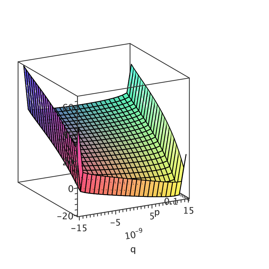
We should also pay attention to choose the initial point $(p,q)$ . Usually, we choose $(0,0)$ and it works well. But there comes troubles for Rump’s problem(see, 4.). When $n=8$ , the iteration for one dimensional search does not converge. Because our methods only converge locally, if $(0,0)$ is too far from the optimizer, the iterations may not converge. If we denote the optimal solution as $(p^{*},q^{*})$ , according to our experiments, we find $p^{*}$ is always attained near the largest feasible value and $q^{*}$ near $0$ (see Figure 1). It is always reasonable since when computing search direction $\delta x$ and $\delta Z$ , we choose method 2, which is based on the primal system only. So we only compute the approximate Newton’s direction of $x$ and choose accessary result $\delta Z^{p}$ of (4) as the dual search direction. So the step length $q$ for $\delta Z$ should be near $0$ . So we choose $(\widehat{p}/2,0)$ as the initial point in plane search where $\widehat{p}$ denotes the largest feasible value of $p$ , and it solves the trouble of Rump’s problem when $n=8$ .

The algorithm PotentialReduction needs initial strictly feasible primal and dual points. We adapt the Big-M method when neither a strictly feasible $x$ nor a strictly feasible $Z$ is known. After modification, the primal problem becomes

$\displaystyle\mathrm{minimize}$	$\displaystyle c^{T}x+\mathit{M_{1}}t$	(6)
$\displaystyle s.t$	$\displaystyle\mathit{F}(x)+t\mathit{I}\geq 0,$
	$\displaystyle\mathbf{Tr}\mathit{F}\leq\mathit{M_{2}},$
	$\displaystyle t\geq 0$

The dual becomes

$\displaystyle\mathrm{maximize}$	$\displaystyle\mathbf{-Tr}\mathit{F_{0}}(Z-z\mathit{I})-\mathit{M_{2}}z$	(7)
$\displaystyle s.t$	$\displaystyle\mathbf{Tr}\mathit{F_{i}}(Z-z\mathit{I})=c_{i},\quad i=1,...,m.$
	$\displaystyle\mathbf{Tr}\mathit{Z}\leq\mathit{M_{1}},$
	$\displaystyle\mathit{Z}\geq 0,z\geq 0$

If $M_{1}$ and $M_{2}$ are big enough, this entails no loss of generality(assuming the primal and dual problem are bounded). After modification, problem (6) and (7) can be written as (1) and (2). Then it is easy to compute its strictly feasible points, see [11]

A brief description of the main functions contained in SDPTools is following:

•

Solution_of_Directions solves the directions $\delta x$ and $\delta Z$ from (4).
•

Expression_of_PlaneSearch gets the objective of (5).
•

StepsLength_PlaneSearch solves problem (5) and get step length $p,q$ for $x,Z$ respectively.
•

BigM_Case3 transforms (6), (7) into (1), (2) respectively, and computes a strict feasible start point $(x_{0},Z_{0})$ .
•

Solve_SDP_Method2 solves the SDP (1) and (2).

3. Certified Global Optimum of Rational Functions

In SDPTools, we apply the SDP algorithm (2.1) to compute and certify the lower bounds of rational functions with rational coefficients.

\displaystyle\min_{\xi\in{\mathbb{R}}^{n}}\frac{f(\xi)}{g(\xi)}\text{\quad(where $g(\xi)>0$ for all $\xi\in{\mathbb{R}}^{n}$)}

(8)

where $f(\xi),g(\xi)\in{\mathbb{Q}}^{n}$ . The number $r$ is a lower bound of (8) if and only if the polynomial $f(x)-rg(x)$ is nonnegative. Therefore we focus on the following minimization of a rational function by SOS:

\left.\begin{aligned} r^{*}:=&\sup_{r\in{\mathbb{R}},W}r\\ s.t&\ f(x)-rg(x)=m_{d}(x)^{T}\cdot W\cdot m_{d}(x)\\ &W\succeq 0,\quad W^{T}=W\end{aligned}\right\}

(9)

where $m_{d}(x)$ is the column vector of all terms in $X_{1},\dots,X_{n}$ up to degree $d$ . A detailed description of SOS relaxations and its dual problems, see [5]. The problem (9) is a semidefinite program and can be written as (2). With packages for solving SDP, we can obtain a numerical positive semidefinite matrix $W$ and floating point number $r^{*}$ which satisfy approximately:

f(x)-r^{*}g(x)\approx m_{d}(x)^{T}\cdot W\cdot m_{d}(x),\ W\succapprox 0

(10)

To certify $r^{*}$ , we convert $r^{*},W$ to rational ones and project orthogonally $W$ onto the affine linear hyperplane:

\displaystyle\chi=\{A|A^{T}

\displaystyle=A,f(x)-rg(x)=m_{d}(x)^{T}\cdot A\cdot m_{d}(x),\quad\text{for some $r$}\}

(11)

and hope $W$ to be positive semidefinte after projection.

However, if we run the fixed precision SDP solver in Matlab, the output $W$ are too coarse to be projected into the cone of positive semidefinite matrices. In [4] they refined the $r^{*},W$ by Gauss-Newton method. Here our high precision SDP solver shows its advantage. It is implemented in Maple, which has arbitrarily high precision, so it can compute $r^{*},W$ with high accuracy. Without refinement, the projection can be done successfully.

Usually, it is not easy to find a strictly feasible point for (9) and we need the Big-M method to avoid it. After convert (9) to the form (7), the SOS relaxation of (8) becomes

\left.\begin{aligned} \widehat{r}^{*}:=\sup_{\widehat{r}\in{\mathbb{R}},\widehat{W}}\quad&\widehat{r}-M_{2}z\\ s.t.\quad&f(x)-\widehat{r}g(x)+z(m_{d}(x)^{T}\cdot m_{d}(x))=m_{d}(x)^{T}\cdot\widehat{W}\cdot m_{d}(x),\\ &\widehat{W}\succeq 0,\quad\widehat{W}^{T}=\widehat{W},\quad z\geq 0\end{aligned}\right\}

(12)

It is obvious to see that problem (9) and (12) are equivalent. And the variable $z$ is required to be $0$ at the optimizer of problem(12). We define

	$\displaystyle\widehat{\chi}=\{\widehat{A}\ \|\ \widehat{A}^{T}$	$\displaystyle=\widehat{A},f(x)-\widehat{r}g(x)+z(m_{d}(x)^{T}\cdot m_{d}(x))$		(13)
		$\displaystyle=m_{d}(x)^{T}\cdot\widehat{A}\cdot m_{d}(x),\quad\text{for some $\widehat{r},z$}\}$		(13)

Note that $\widehat{\chi}$ will meet $\chi$ at the optimizer $(W^{*},r^{*})$ , see Figure 2.

After each iteration, we get a point $(\widehat{r},\widehat{W})$ on $\widehat{\chi}$ . Then we convert $(\widehat{r},\widehat{W})$ to rational ones and project matrix $\widehat{W}$ onto $\chi$ , and denote the nearest matrix in $\chi$ by $\widetilde{W}$ . Because the problem(9) and (12) are equivalent, we can expect that after the first few ones, at each iteration we can obtain a positive semidefinite matrix $\widetilde{W}$ and a certified $r$ . Different from the method in [4] which only certifies a given $r$ , we can get series of certified lower bounds $r_{n}$ . The more iterations we do, the better $r_{n}$ we get. The process is shown in Figure 2.

In order to reduce the problem size, we also exploit sparsity. Given a polynomial $p(x)=\sum_{\alpha}p_{\alpha}x^{\alpha}$ , the cage of $p$ , is the convex hull of $\sup(p)=\{\alpha|\ p_{\alpha}\neq 0\}$ .

Theorem 3.1

([6]) For a polynomial $p$ , $C(p^{2})=2C(p)$ ; for any positive semidefinite polynomial $f$ and $g$ , $C(f)\subseteq C(f+g)$ ; if $f=\sum_{j}g_{j}^{2}$ then $C(g_{j})\subseteq\frac{1}{2}C(f)$ .

With the above theorem, we can remove the redundant monomials in (9).

SDPTools also has functions to compute the convex hull of given finite points in $n$ dimensional vector space. They are mainly based on the Quickhull algorithm in [1] which assumes the affine dimension of the input points is also $n$ . If the affine dimension, denoted by $r$ , is less than $n$ , SDPTools provides a function to compute $r$ and affinely transforms the input points to a $r$ dimensional vector space where we can use the Quickhull algorithm. For a given point, SDPTools has a function to judge whether it is in the convex hull.

SDPTools provides a function to compute the monomials appearing in (9). For example, when solving Rump’s problem, the monomials appearing in $m_{d}(x)$ are obtained by proof in [4] while we can find them automatically by SDPTools!

The followings are the main functions to compute and certify the lower bound of a given rational function:

•

affineDims computes the affine dimension of input points.
•

affineTrans affinely transforms the given points to a $r$ dimensional vector space.
•

convexHull computes the convex hull of given points.
•

inConvexHull judges whether $p$ is in the convex hull defined by the points in $S$ .
•

getSDP transforms problem (9) as form (2).
•

projSOS converts $r,W$ to rational ones and projects $W$ onto $\chi$ .
•

certifiSOS computes and certifies the lower bound of an input rational function.

4. A numerical experiment: solving Rump’s Model Problem

The following introduction to Rump’s model problem (see, [7]) is mostly from [4]. This problem is related to structured condition numbers of Toeplitz matrices and polynomial factor coefficient bounds, asks for $n=1,2,3,\ldots$ to compute the global minima

\begin{array}[]{r@{}@{}l@{}@{}l}\mu_{n}=&\displaystyle\min_{P,\,Q}&\displaystyle\frac{\|PQ\|_{2}^{2}}{\|P\|_{2}^{2}\|Q\|_{2}^{2}}\\[8.61108pt] &\text{s.\ t.\ }&\displaystyle P(z)=\sum_{i=1}^{n}p_{i}z^{i-1},Q(z)=\sum_{i=1}^{n}q_{i}z^{i-1}\in{\mathbb{R}}[z]\setminus\{0\}.\end{array}

It has been shown in [8] that polynomials $P,Q$ realizing the polynomials achieving $\mu_{n}$ must be symmetric (self-reciprocal) or skew-symmetric. Thus the problem can be rewritten into three optimization problems with three different constraints

\begin{array}[]{rlll}k=1\colon&p_{n+1-i}=p_{i},&q_{n+1-i}=q_{i},&1\leq i\leq n,\\ k=2\colon&p_{n+1-i}=p_{i},&q_{n+1-i}=-q_{i},&1\leq i\leq n,\\ k=3\colon&p_{n+1-i}=-p_{i},&q_{n+1-i}=-q_{i},&1\leq i\leq n,\end{array}

and the smallest of three minima is equal to $\mu_{n}$ . For all three cases, we minimize the rational function $f(X)/g(X)$ with

\begin{array}[]{l@{}@{}l}f(X)&\displaystyle{}=\|PQ\|_{2}^{2}=\sum_{k=2}^{2n}(\sum_{i+j=k}p_{i}q_{j})^{2},\quad g(X)\displaystyle{}=\|P\|_{2}^{2}\|Q\|_{2}^{2}=(\sum_{i=1}^{n}p_{i}^{2})(\sum_{j=1}^{n}q_{j}^{2})\end{array}

and the variables $X=\{p_{1},\ldots,p_{n(P)}\}\cup\{q_{1},\ldots,q_{n(Q)}\},$ where $n(P)=n(Q)=\lceil{n}/{2}\rceil$ .

In this paper, we use higher precision SDP solver in SDPTools to solve Rump’s model problem and obtain much better certified lower bounds, see Table 1.

$n$ $k$ # iter prec. secs/iter lower bound $r_{n}$ upper bound 4 2 50 4 $\times$ 15 0.71 0.01742917332143265287 0.01742917332143265289 5 1 50 4 $\times$ 15 2.03 0.00233959554815559112 0.00233959554815559113 6 2 50 4 $\times$ 15 1.76 0.00028973187527968191 0.00028973187527968193 7 1 75 5 $\times$ 15 11.36 0.00003418506980008284 0.00003418506980008285 8 2 75 5 $\times$ 15 12.49 0.00000390543564975572 0.00000390543564975573 9 1 75 5 $\times$ 15 84.12 0.43600165391810484612e-06 0.43600165391810484613e-06 10 2 75 5 $\times$ 15 92.79 0.47839395687709759326e-07 0.47839395687709759327e-07 11 1 85 5 $\times$ 15 622.03 0.51787490974469905330e-08 0.51787490974469908331e-08 12 2 85 5 $\times$ 15 634.48 0.55458818311631347611e-09 0.55458818311631347612e-09 13 1 100 5 $\times$ 15 3800.0 0.58866880811866093129e-10 0.58866880811866093130e-10 14 2 100 5 $\times$ 15 3800.0 0.62024449920539050219e-11 0.62024449920539050220e-11 15 1 120 6 $\times$ 15 15000 0.64943654185809512879e-12 0.64943654185809512880e-12 16 2 120 6 $\times$ 15 23000 0.67636042558221379057e-13 0.67636042558221379058e-13

Table 1: The certified lower bounds

5. Conclusion

SDPTools is a Maple package having the following functions: to solve a general SDP, to compute and certify the lower bounds of rational functions. It is also a tool to compute the convex hull of given finite points in order to explore the sparsity structure.

SDPTools is still under development, we hope to implement more efficient algorithms to solve SDP, to give upper bounds for $M_{1},M_{2}$ when applying Big-M method in SOS relaxation (12), to detect the infeasibility for SDP and to explore more sparsity structures for problems having large size.

References

[1] C. Bradford Barber, David P. Dobkin, and Hannu Huhdanpaa. The quickhull algorithm for convex hulls. ACM Transactions on Mathematical Software, 22(4):469–483, December 1996.
[2] Steven J. Benson and Yinyu Ye. DSDP5: Software for semidefinite programming. Technical Report ANL/MCS-P1289-0905, Mathematics and Computer Science Division, Argonne National Laboratory, Argonne, IL, September 2005. Submitted to ACM Transactions on Mathematical Software.
[3] Katsuki Fujisawa, Masakazu Kojima, and Kazuhide Nakata. Sdpa (semidefinite programming algorithm) user manual - version 4.10. Technical report, 1998.
[4] Erich Kaltofen, Bin Li, Zhengfeng Yang, and Lihong Zhi. Exact certification of global optimality of approximate factorizations via rationalizing sums-of-squares with floating point scalars. In ISSAC ’08: Proceedings of the twenty-first international symposium on Symbolic and algebraic computation, pages 155–164, New York, NY, USA, 2008. ACM.
[5] Jiawang Nie, James Demmel, and Ming Gu. Global minimization of rational functions and the nearest gcds. J. of Global Optimization, 40(4):697–718, 2008.
[6] Bruce Reznick. Extremal PSD forms with few terms. Duke Mathematical Journal, 45(2):363–374, 1978.
[7] Siegfried M. Rump. Global optimization: a model problem, 2006. URL: http://www.ti3.tu-harburg.de/rump/Research/ModelProblem.pdf.
[8] Siegfried M. Rump and H. Sekigawa. The ratio between the Toeplitz and the unstructured condition number, 2006. To appear. URL: http://www.ti3.tu-harburg.de/paper/rump/RuSe06.pdf.
[9] Jos F. Sturm. Using SeDuMi 1.02, a MATLAB toolbox for optimization over symmetric cones. Optimization Methods and Software, 11/12:625–653, 1999.
[10] K. C. Toh, M. J. Todd, R. H. T¨¹t¨¹nc¨¹, and R. H. Tutuncu. Sdpt3 - a matlab software package for semidefinite programming. Optimization Methods and Software, 11:545–581, 1998.
[11] Lieven Vandenberghe and Stephen Boyd. Semidefinite programming. SIAM Review, 38(1):49–95, 1996.