Constructing families of elliptic curves with prescribed mod $3$ representation via Hessian and Cayleyan curvesThanks: After submitting the first version of this paper on the arXiv, the author was informed that the main observation of this paper had already been made by Tom Fisher, The Hessian of a genus one curve, Proc. Lond. Math. Soc. (3) 104 (2012), 613-648.

Masato Kuwata Address: Faculty of Economics, Chuo University, 742-1 Higashinakano, Hachioji-shi, Tokyo 192-0393, Japan Email address: kuwata@tamacc.chuo-u.ac.jp

1. Introduction

Let $E_{0}$ be an elliptic curve defined over a number field $k$ . The subgroup of $3$ -torsion points $E_{0}[3]$ of $E_{0}(\bar{k})$ is a Galois module that gives rise to a representation

\bar{\rho}_{E_{0},3}:\operatorname{Gal}(\bar{k}/k)\to\operatorname{Aut}(E_{0}[3])\cong GL_{2}(\mathbb{F}_{3}).

The collection of elliptic curves over $k$ having the same mod $3$ representation as a given elliptic curve $E_{0}$ forms an infinite family. In this paper we give an explicit construction of this family using the notion Hessian and Cayleyan curves in classical geometry.

Suppose $\phi:E_{0}[3]\to E[3]$ is an isomorphism as Galois modules. Then, either $\phi$ commutes with the Weil pairings $e_{E_{0},3}$ and $e_{E,3}$ , or we have

e_{E,3}\bigl(\phi(P),\phi(Q)\bigr)=e_{E_{0},3}(P,Q)^{-1}

for all $P,Q\in E_{0}[3]$ . In the former case, we call $\phi$ a symplectic isomorphism, or an isometry. In the latter case, we call $\phi$ an anti-symplectic isomorphism, or an anti-isometry.

Rubin and Silverberg [6] gave an explicit construction of the family of elliptic curves $E$ over $k$ that admits a symplectic isomorphism $E_{0}[3]\to E[3]$ . There is a universal elliptic curve $\mathcal{E}_{t}$ over a twist of noncompact modular curve $Y_{3}$ which is a twist of the Hesse cubic curve $x^{3}+y^{3}+z^{3}=3\lambda xyz.$ We give an alternative construction of this family using the Hessian curve of $E_{0}$ (see §2 for definition). The family of elliptic curves $F$ over $k$ that admits a anti-symplectic isomorphism $E_{0}[3]\to F[3]$ is related to the construction of curves of genus $2$ that admit a morphism of degree $3$ to $E_{0}$ (see Frey and Kani [4]). We show that there is a universal elliptic curve $\mathcal{F}_{t}$ for this family, and we give a construction using the Caylean curves (see §3) in the dual projective plane.

Our main results are roughly as follows. Choose a model of $E_{0}$ as a plane cubic curve such that the origin $O$ of the group structure of $E_{0}$ is an inflection point. A Weierstrass model of $E_{0}$ satisfies this condition. Then, its Hessian curve $\operatorname{{\it He}}(E_{0})$ is a cubic curve in the same projective plane and the intersection $E_{0}\cap\operatorname{{\it He}}(E_{0})$ is nothing but the group of $3$ -torsion points. We will show that the pencil of cubic curves

\mathcal{E}_{t}:E_{0}+t\operatorname{{\it He}}(E_{0})

is nothing but the family with symplectic isomorphism $E_{0}[3]\to\mathcal{E}_{t}[3]$ , as the nine base points of the pencil form the subgroup $\mathcal{E}_{t}[3]$ for each $t$ (Theorem 4.2).

It is classically known that the Hessian curve $\operatorname{{\it He}}(E)$ admits a fixed point free involution $\iota$ (see [1][3]). The line joining the points $P$ and $\iota(P)$ , denoted by $\overline{P\iota(P)}$ , gives a point in the dual projective plane $(\mathbf{P}^{2})^{*}$ . The locus of such lines $\overline{P\iota(P)}$ for all $P\in E_{0}$ is a cubic curve in $(\mathbf{P}^{2})^{*}$ classically known as Cayleyan curve and it is denoted by $\operatorname{{\it Ca}}(E_{0})$ . It is easy to see that $\operatorname{{\it Ca}}(E_{0})$ is isomorphic to the quotient $\operatorname{{\it He}}(E_{0})/\langle\iota\rangle$ , and we can prove that the map associating $P\in E_{0}[3]$ to its inflection tangent $T_{P}\in\operatorname{{\it Ca}}(E_{0})[3]$ is an anti-symplectic isomorphism. Since $\operatorname{{\it Ca}}(E_{0})$ also has a fixed point free involution, we may expect that it is the Hessian of a cubic curve in $(\mathbf{P}^{2})^{*}$ , and it turns out this is the case. There is a cubic curve $F_{0}$ in $(\mathbf{P}^{2})^{*}$ whose Hessian is $\operatorname{{\it Ca}}(E_{0})$ . The pencil of cubic curves

\mathcal{F}_{t}:F_{0}+t\operatorname{{\it Ca}}(E_{0})

is then the family with anti-symplectic isomorphism $E_{0}[3]\to\mathcal{F}_{t}[3]$ .

If $E_{0}$ is given by the Weierstrass equation

E_{0}:y^{2}z=x^{3}+Axz^{2}+Bz^{3},

then the equations of $\operatorname{{\it He}}(E_{0})$ , $\operatorname{{\it Ca}}(E_{0})$ , and $F_{0}$ are given by

\begin{array}[]{ccl}\operatorname{{\it He}}(E_{0})&:&3Ax^{2}z+9Bxz^{2}+3xy^{2}-A^{2}z^{3}=0,\\ \operatorname{{\it Ca}}(E_{0})&:&A\xi^{3}+9B\xi\eta^{2}+3\xi\zeta^{2}-6A\eta^{2}\zeta=0,\\ F_{0}&:&AB\xi^{3}-2A^{2}\xi^{2}\zeta-(4A^{3}+27B^{2})\xi\eta^{2}-9B\xi\zeta^{2}+2A\zeta^{3}=0,\end{array}

where $(\xi:\eta:\zeta)$ is the dual coordinate of $(\mathbf{P}^{2})^{*}$ .

In §6 we give some applications. From our description of $\mathcal{E}_{t}$ and $\mathcal{F}_{t}$ , it is clear that the elliptic surfaces associated to these families are rational elliptic surfaces over $k$ . As a consequence, we are able to apply Salgado’s theorem [7] to our family (Theorem 6.1).

Let $F$ be a nonsingular member of $\mathcal{F}_{t}$ . Since we have an anti-symplectic isomorphism $\psi:E_{0}[3]\to F[3]$ , Frey and Kani [4] show that there exists a curve $C$ of genus $2$ that admits two morphism $C\to E_{0}$ and $C\to F$ of degree $3$ . Indeed, the quotient of $E_{0}\times F$ by the graph of $\psi$ is a principally polarized abelian surface that is the Jacobian of a curve $C$ of genus $2$ . For example, if we take $\operatorname{{\it Ca}}(E_{0})$ as $F$ , then it turns out that this is the degenerate case where $C\to\operatorname{{\it Ca}}(E_{0})$ is ramified at one place with ramification index $3$ . We will give explicit formulas for this case (Proposition 6.2).

2. Hessian of a plane cubic

Let $C$ be a plane curve defined by a homogenous equation $F(x,y,z)=0$ . In this section we summarize some facts on polarity, with a special emphasis on our particular case of cubic curves. In this section and the next, the base filed is taken as an algebraic closure of $k$ . For more general treatment, see Dolgachev [3, Ch. 1 and Ch. 3].

For a nonzero vector $\boldsymbol{a}={}^{t}(a_{0},a_{1},a_{2})$ , we define the differential operator $\nabla_{\boldsymbol{a}}$ by

\nabla_{\boldsymbol{a}}=a_{0}\frac{\partial}{\partial x}+a_{1}\frac{\partial}{\partial y}+a_{2}\frac{\partial}{\partial z}.

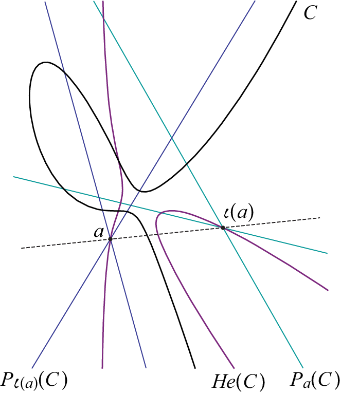
Here, $\nabla_{\boldsymbol{a}}F(x,y,z)$ stands for the directional derivative of $F(x,y,z)$ along the direction vector $\boldsymbol{a}$ . The first polar curve of $C$ is then defined by the equation $\nabla_{\boldsymbol{a}}F(x,y,z)=0$ . It depends only on the point $a=(a_{0}:a_{1}:a_{2})\in\mathbf{P}^{2}$ , but not the vector $\boldsymbol{a}$ itself. Thus, we denote the first polar curve by $P_{a}(C)$ :

P_{a}(C):\nabla_{\boldsymbol{a}}F(x,y,z)=0.

When $C$ is a cubic, $P_{a}(C)$ is a conic.

Refer to caption — Figure 1. First polar curve

Also, the second polar curve of $C$ is defined by $\nabla_{\boldsymbol{a}}\nabla_{\boldsymbol{a}}F(x,y,z)=0$ . The composition of differential operators $\nabla_{\boldsymbol{a}}\circ\nabla_{\boldsymbol{a}}$ is sometimes denote by $\nabla_{\boldsymbol{a}^{2}}$ , and thus the second polar is denoted by $P_{a^{2}}(C)$ :

P_{a^{2}}(C):\nabla_{\boldsymbol{a}^{2}}F(x,y,z)=0.

When $C$ is a cubic, $P_{a^{2}}(C)$ is a line.

In general we define the differential operator $\nabla_{\boldsymbol{a}^{k}}$ inductively by

\nabla_{\boldsymbol{a}^{k}}=\nabla_{\boldsymbol{a}}\circ\nabla_{\boldsymbol{a}^{k-1}},\quad k\geq 2,

and for a plane curve $C$ of any degree, the $k$ -th polar $P_{a^{k}}(C)$ is defined by

P_{a^{k}}(C):\nabla_{\boldsymbol{a}^{k}}F(x,y,z)=0.

With this notation the Taylor expansion formula for a general analytic function $F$ can be written in the following form:

	$\displaystyle F(\boldsymbol{x}+\boldsymbol{a})$	$\displaystyle=\sum_{k=0}^{\infty}\frac{1}{k!}\nabla_{\boldsymbol{a}^{k}}F(\boldsymbol{x})$
		$\displaystyle=F(\boldsymbol{x})+\nabla_{\boldsymbol{a}}F(\boldsymbol{x})+\frac{1}{2!}\nabla_{\boldsymbol{a}^{2}}F(\boldsymbol{x})+\frac{1}{3!}\nabla_{\boldsymbol{a}^{3}}F(\boldsymbol{x})+\cdots,$

where $\boldsymbol{x}={}^{t}(x,y,z)$ . With matrix notation we can write

\nabla_{\boldsymbol{a}}F(\boldsymbol{x})=F^{\prime}(\boldsymbol{x})\boldsymbol{a},\quad\nabla_{\boldsymbol{b}}\nabla_{\boldsymbol{a}}F(\boldsymbol{x})={}^{t}\boldsymbol{b}F^{\prime\prime}(\boldsymbol{x})\boldsymbol{a}.

where

F^{\prime}(\boldsymbol{x})=\begin{pmatrix}F_{x}(\boldsymbol{x})&F_{y}(\boldsymbol{x})&F_{z}(\boldsymbol{x})\end{pmatrix},\quad F^{\prime\prime}(\boldsymbol{x})=\begin{pmatrix}F_{xx}(\boldsymbol{x})&F_{xy}(\boldsymbol{x})&F_{xz}(\boldsymbol{x})\\ F_{yx}(\boldsymbol{x})&F_{yy}(\boldsymbol{x})&F_{yz}(\boldsymbol{x})\\ F_{zx}(\boldsymbol{x})&F_{zy}(\boldsymbol{x})&F_{zz}(\boldsymbol{x})\end{pmatrix}.

Here $F_{x}(\boldsymbol{x})$ and $F_{xx}(\boldsymbol{x})$ , for example, mean partial derivative $\frac{\partial F}{\partial x}(x,y,z)$ and the second partial derivative $\frac{\partial^{2}F}{\partial x^{2}}(x,y,z)$ . The $3\times 3$ matrix $F^{\prime\prime}(\boldsymbol{x})$ is called the Hessian matrix, and is sometimes denoted by $\operatorname{{\it He}}(F)(\boldsymbol{x})$ .

Definition 2.1.

The Hessian $\operatorname{{\it He}}(C)$ of $C$ is defined by

\operatorname{{\it He}}(C):\det F^{\prime\prime}(\boldsymbol{x})=\left|\begin{matrix}F_{xx}(\boldsymbol{x})&F_{xy}(\boldsymbol{x})&F_{xz}(\boldsymbol{x})\\ F_{yx}(\boldsymbol{x})&F_{yy}(\boldsymbol{x})&F_{yz}(\boldsymbol{x})\\ F_{zx}(\boldsymbol{x})&F_{zy}(\boldsymbol{x})&F_{zz}(\boldsymbol{x})\end{matrix}\right|=0.

Remark 2.2.

The determinant $\det F^{\prime\prime}(\boldsymbol{x})$ can be identically zero. For example, if $C$ is defined by $F(x,y,z)=xy^{2}+zy^{2}$ , then $\det F^{\prime\prime}(\boldsymbol{x})=0$ identically. In this case we have $\operatorname{{\it He}}(C)=\mathbf{P}^{2}$ .

To see the meaning of $P_{a^{k}}(C)$ , let $a=(a_{0}:a_{1}:a_{2})$ and $b=(b_{0}:b_{1}:b_{2})$ be two points in $\mathbf{P}^{2}$ , and let $\ell=\overline{ab}$ be the line joining the two points. $\ell$ is the image of the map $\lambda:\mathbf{P}^{1}\to\mathbf{P}^{2}$

\lambda:(s:t)\mapsto sa+tb=(sa_{0}+tb_{0}:sa_{1}+tb_{1}:sa_{2}+tb_{2}).

If the degree of $F$ is $n$ , then the Taylor expansion formula around the point $(s:t)=(1:0)$ gives a homogenous polynomial of degree $n$ in $s$ and $t$ :

(2.1)

F(s\boldsymbol{a}+t\boldsymbol{b})=\\ F(\boldsymbol{a})s^{n}+\nabla_{\boldsymbol{b}}F(\boldsymbol{a})s^{n-1}t+\frac{1}{2!}\nabla_{\boldsymbol{b}^{2}}F(\boldsymbol{a})s^{n-2}t^{2}+\frac{1}{3!}\nabla_{\boldsymbol{b}^{3}}F(\boldsymbol{a})s^{n-3}t^{3}+\cdots.

Before going further, we need a few lemmas.

Lemma 2.3.

Let $Q$ be a plane conic defined by ${}^{t}\boldsymbol{x}M\boldsymbol{x}=0$ , where $M$ is a symmetric matrix. Let $a=(a_{0}:a_{1}:a_{2})$ be a point on $Q$ , and $\boldsymbol{a}={}^{t}(a_{0},a_{1},a_{2})$ is the corresponding vector.

(1)

$a$ is a singular point if and only if $M\boldsymbol{a}=\boldsymbol{0}$ .
(2)

$Q$ is degenerate if and only if $\det M=0$ .
(3)

If $a$ is a smooth point, then the tangent line $T_{a}(Q)$ at $a$ is given by the equation ${}^{t}\boldsymbol{x}M\boldsymbol{a}=0$ .

Proof.

Let $b$ be a point in $\mathbf{P}^{2}$ different from $a$ . The intersection between the line $\overline{ab}$ and $Q$ is given by the solution $(s:t)$ to the equation

(2.2)

{}^{t}(s\boldsymbol{a}+t\boldsymbol{b})M(s\boldsymbol{a}+t\boldsymbol{b})=2({}^{t}\boldsymbol{b}M\boldsymbol{a})st+({}^{t}\boldsymbol{b}M\boldsymbol{b})t^{2}=0.

The point $a$ is a singular point of $Q$ if and only if the multiplicity of intersection $\overline{ab}\cap Q$ at $a$ is greater than $1$ for any point $b$ in $\mathbf{P}^{2}$ . This is equivalent to say that ${}^{t}\boldsymbol{b}M\boldsymbol{a}=0$ for any $\boldsymbol{b}$ . This condition in turn is equivalent to the condition $M\boldsymbol{a}=\boldsymbol{0}$ .

The curve $Q$ is degenerate if and only if it has a singular point. This is equivalent to the existence of a nonzero vector $\boldsymbol{a}$ satisfying $M\boldsymbol{a}=\boldsymbol{0}$ , which in turn is equivalent to the condition $\det M=0$ .

A point $b$ is on the tangent line $T_{a}$ if and only if $\overline{ab}$ intersects with $Q$ at $a$ with multiplicity $2$ . The equation (2.2) shows that the latter condition is equivalent to the condition that $b$ satisfies the equation ${}^{t}\boldsymbol{x}M\boldsymbol{a}=0$ . Thus, the equation of the tangent line $T_{a}$ is given by ${}^{t}\boldsymbol{x}M\boldsymbol{a}=0$ . ∎

Lemma 2.4 (Euler’s formula).

Let $F(\boldsymbol{x})$ be a homogeneous polynomial of degree $d$ , where $\boldsymbol{x}={}^{t}(x_{0},x_{1},\dots,x_{n})$ . Then, we have

d(d-1)\dots(d-k+1)F(\boldsymbol{x})=\nabla_{\boldsymbol{x}^{k}}F(\boldsymbol{x}).

Proof.

Since $F$ is homogeneous of degree $d$ , we have $F(\lambda\boldsymbol{x})=\lambda^{d}F(\boldsymbol{x})$ . Take its $k$ th derivative with respect to $\lambda$ and put $\lambda=1$ . ∎

Proposition 2.5.

Let $C$ be a plane curve of degree $d$ defined by a homogeneous equation $F(\boldsymbol{x})=0$ . Suppose that $a$ is a smooth (simple) point of $C$ .

(1)

For any point $b$ in $\mathbf{P}^{2}$ different from $a$ , the line $\ell=\overline{ab}$ is tangent to $C$ at $a$ if and only if $a\in C\cap P_{b}(C)$ . (See Figure 1.)
(2)

The equation of the tangent line $T_{a}(C)$ at $a$ is given by

$\nabla_{\boldsymbol{x}}F(\boldsymbol{a})=0,\quad\text{or}\quad F^{\prime}(\boldsymbol{a})\boldsymbol{x}=0.$
(3)

$P_{a}(C)$ is tangent to $C$ at $a$ .
(4)

$a$ is an inflection point if and only if $a\in C\cap\operatorname{{\it He}}(C)$ .

Proof.

(1) The line $\ell=\overline{ab}$ is tangent to $C$ at $a$ if and only if the multiplicity of intersection at $a\in\ell\cap C$ is at least two. By (2.1), this is equivalent to the condition $F(\boldsymbol{a})=0$ and $\nabla_{\boldsymbol{b}}F(\boldsymbol{a})=0$ . This in turn is equivalent to the condition $a\in C\cap P_{b}(C)$ .

(2) A point $b$ is on the tangent line $T_{a}(C)$ if and only if $\ell=\overline{ab}$ is tangent to $C$ at $a$ . By the proof of (1), the latter is equivalent to $\nabla_{\boldsymbol{b}}F(\boldsymbol{a})=0$ . Thus, $\nabla_{\boldsymbol{x}}F(\boldsymbol{a})=0$ is the equation of $T_{a}(C)$

(3) By Euler’s formula, $F(\boldsymbol{a})=0$ implies $\nabla_{\boldsymbol{a}}F(\boldsymbol{a})=0$ . Thus, $P_{a}(C)$ passes through $a$ . Suppose $b$ is on $T_{a}(C)$ . Then, we have $\nabla_{\boldsymbol{b}}F(\boldsymbol{a})=0$ by (2). We would like to show that $\overline{ab}$ is also tangent to $P_{a}(C)$ . Applying Euler’s formula to the polynomial $\nabla_{\boldsymbol{b}}F(\boldsymbol{x})$ of degree $d-1$ , we have

\nabla_{\boldsymbol{x}}(\nabla_{\boldsymbol{b}}F)(\boldsymbol{x})=(d-1)\nabla_{\boldsymbol{b}}F(\boldsymbol{x}).

Using the formula $\nabla_{\boldsymbol{x}}(\nabla_{\boldsymbol{b}}F)(\boldsymbol{x})=\nabla_{\boldsymbol{b}}(\nabla_{\boldsymbol{x}}F)(\boldsymbol{x})$ and replacing $\boldsymbol{x}$ by $\boldsymbol{a}$ , we obtain

\nabla_{\boldsymbol{b}}(\nabla_{\boldsymbol{a}}F)(\boldsymbol{a})=(d-1)\nabla_{\boldsymbol{b}}F(\boldsymbol{a})=0.

This implies that $b$ is tangent at $a$ to the curve defined by $\nabla_{\boldsymbol{a}}F(\boldsymbol{x})=0$ , which is nothing but $P_{a}(C)$ .

(4) The line $\ell=\overline{ab}$ is an inflection tangent to $C$ at $a$ if and only if $F(\boldsymbol{a})=\nabla_{\boldsymbol{b}}F(\boldsymbol{a})=\nabla_{\boldsymbol{b}^{2}}F(\boldsymbol{a})=0$ . Thus, if $T_{a}(C)$ is an inflection tangent, any point $b\in T_{a}(C)$ satisfies the condition $\nabla_{\boldsymbol{b}^{2}}F(\boldsymbol{a})=0$ . This implies that the tangent line $\nabla_{\boldsymbol{x}}F(\boldsymbol{a})=0$ is contained in the curve defined by $\nabla_{\boldsymbol{x}^{2}}F(\boldsymbol{a})=0$ as a component. Since $\nabla_{\boldsymbol{x}^{2}}F(\boldsymbol{a})={}^{t}\boldsymbol{x}F^{\prime\prime}(\boldsymbol{a})\boldsymbol{x}$ , $\nabla_{\boldsymbol{x}^{2}}F(\boldsymbol{a})=0$ is a conic, and this conic is degenerate if and only if $\det F^{\prime\prime}(\boldsymbol{a})=0$ by Lemma 2.3(2). Thus, $a\in C\cap\operatorname{{\it He}}(C)$ .

Conversely, suppose $a\in C\cap\operatorname{{\it He}}(C)$ . Since $\det F^{\prime\prime}(\boldsymbol{a})=0$ , the conic $\nabla_{\boldsymbol{x}^{2}}F(\boldsymbol{a})=0$ is degenerate. This conic passes through $a$ since $\nabla_{\boldsymbol{a}^{2}}F(\boldsymbol{a})=d(d-1)F(\boldsymbol{a})=0$ by Euler’s formula (Lemma 2.4). Also, the tangent line $T_{a}(C):\nabla_{\boldsymbol{x}}F(\boldsymbol{a})=0$ is contained in the degenerate conic $\nabla_{\boldsymbol{x}^{2}}F(\boldsymbol{a})=0$ . This is because the tangent line to this conic at $a$ is given by ${}^{t}\boldsymbol{x}F^{\prime\prime}(\boldsymbol{a})\boldsymbol{a}=0$ by Lemma 2.3(3), and ${}^{t}\boldsymbol{x}F^{\prime\prime}(\boldsymbol{a})\boldsymbol{a}=\nabla_{\boldsymbol{a}}\nabla_{\boldsymbol{x}}F(\boldsymbol{a})=(d-1)\nabla_{\boldsymbol{x}}F(\boldsymbol{a})$ again by Euler’s formula (applied to the polynomial $\nabla_{\boldsymbol{x}}F(\boldsymbol{\boldsymbol{y}})$ of degree $d-1$ in $\boldsymbol{y}$ ). Thus, $T_{a}(C)$ is an inflection tangent and $a$ is an inflection point. ∎

From now on we focus on the case where $C$ is a cubic curve. In this case the Taylor expansion formula around the point $(s:t)=(1:0)$ gives a homogenous cubic polynomial in $s$ and $t$ :

(2.3)

F(s\boldsymbol{a}+t\boldsymbol{b})=F(\boldsymbol{a})s^{3}+\nabla_{\boldsymbol{b}}F(\boldsymbol{a})s^{2}t+\frac{1}{2!}\nabla_{\boldsymbol{b}^{2}}F(\boldsymbol{a})st^{2}+\frac{1}{3!}\nabla_{\boldsymbol{b}^{3}}F(\boldsymbol{a})t^{3}.

Exchanging the roles of $\boldsymbol{a}$ and $\boldsymbol{b}$ in (2.3), that is, using the Taylor expansion formula around the point $(s:t)=(0:1)$ , we have another form of expansion:

(2.4)

F(s\boldsymbol{a}+t\boldsymbol{b})=F(\boldsymbol{b})t^{3}+\nabla_{\boldsymbol{a}}F(\boldsymbol{b})st^{2}+\frac{1}{2!}\nabla_{\boldsymbol{a}^{2}}F(\boldsymbol{b})s^{2}t+\frac{1}{3!}\nabla_{\boldsymbol{a}^{3}}F(\boldsymbol{b})s^{3}.

Comparing the corresponding coefficients in (2.3) and (2.4), we have

(2.5)

\begin{gathered}F(\boldsymbol{a})=\frac{1}{3!}\nabla_{\boldsymbol{a}^{3}}F(\boldsymbol{b}),\qquad\nabla_{\boldsymbol{b}}F(\boldsymbol{a})=\frac{1}{2!}\nabla_{\boldsymbol{a}^{2}}F(\boldsymbol{b}),\\ \frac{1}{2!}\nabla_{\boldsymbol{b}^{2}}F(\boldsymbol{a})=\nabla_{\boldsymbol{a}}F(\boldsymbol{b}),\qquad\frac{1}{3!}\nabla_{\boldsymbol{b}^{3}}F(\boldsymbol{a})=F(\boldsymbol{b}).\end{gathered}

With matrix notation the second and the third relation may be written as follows:

(2.6)

\displaystyle F^{\prime}(\boldsymbol{a})\boldsymbol{b}=\frac{1}{2!}\left({}^{t}\boldsymbol{a}F^{\prime\prime}(\boldsymbol{b})\boldsymbol{a}\right),\quad\frac{1}{2!}\left({}^{t}\boldsymbol{b}F^{\prime\prime}(\boldsymbol{a})\boldsymbol{b}\right)=F^{\prime}(\boldsymbol{b})\boldsymbol{a}.

Proposition 2.6.

Let $C$ be a plane cubic curve defined by an equation $F(\boldsymbol{x})=0$ .

(1)

If $a$ is a smooth point of $C$ , then the equation of the tangent line $T_{a}(C)$ at $a$ may be written in two different forms

$\nabla_{\boldsymbol{x}}F(\boldsymbol{a})=0,\quad\text{and}\quad\nabla_{\boldsymbol{a^{2}}}F(\boldsymbol{x})=0.$

In particular, the second polar $P_{a^{2}}(C)$ of $C$ is the tangent line $T_{a}(C)$ .
(2)

If $a$ is a singular point of $C$ , then $P_{a^{2}}(C)$ coincides with $\mathbf{P}^{2}$ .

Proof.

(1) By Proposition 2.5(2), $\nabla_{\boldsymbol{x}}F(\boldsymbol{a})=0$ is the equation of $T_{a}(C)$ . By (2.5) this equation is equivalent to $\nabla_{\boldsymbol{a^{2}}}F(\boldsymbol{x})=0$ . But, this is nothing but the equation of the second polar $P_{a^{2}}(C)$ , and thus, $P_{a^{2}}(C)$ coincides with $T_{a}$ .

(2) If $a$ is a singular point, the multiplicity of the intersection $\overline{ab}\cap C$ at $a$ is always greater than $1$ . It follows from (2.3) that for any point $b\in\mathbf{P}^{2}$ , $\nabla_{\boldsymbol{b}}F(\boldsymbol{a})=0$ . Then, by (2.5), we have $\nabla_{\boldsymbol{a^{2}}}F(\boldsymbol{b})=0$ for any $b\in\mathbf{P}^{2}$ , which implies $P_{a^{2}}(C)=\mathbf{P}^{2}$ . ∎

Proposition 2.7.

Let $C$ be a plane cubic curve. Suppose that the Hessian $\operatorname{{\it He}}(C)$ does not coincide with $\mathbf{P}^{2}$ .

(1)

A point $a\in\mathbf{P}^{2}$ is on $\operatorname{{\it He}}(C)$ if and only if the first polar $P_{a}(C)$ is degenerate.
(2)

Suppose $a$ is on $\operatorname{{\it He}}(C)$ . Let $b$ be a singular point of the degenerated first polar $P_{a}(C)$ . Then, $b$ is again on $\operatorname{{\it He}}(C)$ , and $a$ is a singular point of $P_{b}(C)$ .

Proof.

(1) Using (2.5), we see that the equation of $P_{a}(C)$ can also be written in the form

(2.7)

\nabla_{\boldsymbol{x}^{2}}F(\boldsymbol{a})={}^{t}\boldsymbol{x}F^{\prime\prime}(\boldsymbol{a})\boldsymbol{x}=0.

Thus, $P_{a}(C)$ is degenerate if and only if $\det F^{\prime\prime}(\boldsymbol{a})=0$ .

(2) If $a\in\operatorname{{\it He}}(C)$ , it follows from (1) that $P_{a}(C)$ has a singular point. The first polar $P_{a}(C)$ is defined by the equation $\nabla_{\boldsymbol{a}}F(\boldsymbol{x})=0$ . By the Jacobian criterion, a singular point of $P_{a}(C)$ is a solution of the system of equations

\frac{\partial}{\partial x}\nabla_{\boldsymbol{a}}F(\boldsymbol{x})=\frac{\partial}{\partial y}\nabla_{\boldsymbol{a}}F(\boldsymbol{x})=\frac{\partial}{\partial z}\nabla_{\boldsymbol{a}}F(\boldsymbol{x})=0.

With matrix notation these equations can be combined into one equation

(2.8)

F^{\prime\prime}(\boldsymbol{x})\boldsymbol{a}=\boldsymbol{0}.

Now, if $b=(b_{0}:b_{1}:b_{2})$ is a singular point of $P_{a}(C)$ , then $\boldsymbol{b}={}^{t}(b_{0},b_{1},b_{2})$ satisfies the equation (2.8), that is, we have $F^{\prime\prime}(\boldsymbol{b})\boldsymbol{a}=\boldsymbol{0}$ . This, in particular, implies that $\det F^{\prime\prime}(\boldsymbol{b})=0$ . This shows $b\in\operatorname{{\it He}}(C)$ .

Meanwhile, $P_{b}(C)$ is given by the equation ${}^{t}\boldsymbol{x}F^{\prime\prime}(\boldsymbol{b})\boldsymbol{x}=0$ just as $P_{a}(C)$ is given by (2.7). Thus, by Lemma 2.3, a singular point of such a conic is a solution of the equation

(2.9)

F^{\prime\prime}(\boldsymbol{b})\boldsymbol{x}=\boldsymbol{0}.

Then, the condition $F^{\prime\prime}(\boldsymbol{b})\boldsymbol{a}=\boldsymbol{0}$ can be interpreted that $\boldsymbol{a}$ satisfies the equation (2.9). This implies that $a$ is a singular point of $P_{b}(C)$ . ∎

Proposition 2.8.

Let $C$ be a plane cubic curve. Suppose that the Hessian $\operatorname{{\it He}}(C)$ is a nonsingular cubic curve.

(1)

If $a$ is on $\operatorname{{\it He}}(C)$ , then $P_{a}(C)$ is the union of two distinct lines.
(2)

The map that associates $a\in\operatorname{{\it He}}(C)$ to the unique singular point $b$ of $P_{a}(C)$ determines an involution $\iota$ on $\operatorname{{\it He}}(C)$ without fixed points.
(3)

If $a\in C\cap\operatorname{{\it He}}(C)$ , then the inflection tangent line $T_{a}(C)$ is contained as a component in the degenerated first polar curve $P_{a}(C)$ .

Proof.

(1) If $a$ is on $\operatorname{{\it He}}(C)$ and $P_{a}(C)$ is a double line or the entire plane, then all the points $b$ on $P_{a}(C)$ are singular points. Then, by Proposition 2.7 (2), $b$ is on $\operatorname{{\it He}}(C)$ . This means $P_{a}(C)$ is contained in $\operatorname{{\it He}}(C)$ as a component. This contradicts the assumption that $\operatorname{{\it He}}(C)$ is nonsingular.

(2) Proposition 2.7 (2) shows that the map $\iota$ described in the statement is indeed an involution. It only remains to prove that this involution does not have any fixed point. If $a$ is a fixed point of $\iota$ , then $a$ is the singular point of $P_{a}(C)$ . Since $P_{a}(C)$ is a conic given by ${}^{t}\boldsymbol{x}F^{\prime\prime}(\boldsymbol{a})\boldsymbol{x}=0$ , this implies $F^{\prime\prime}(\boldsymbol{a})\boldsymbol{a}=\boldsymbol{0}$ by Lemma 2.3(1). In general, for a conic $Q$ given by ${}^{t}\boldsymbol{x}M\boldsymbol{x}=0$ with a symmetric matrix $M$ , its first polar $P_{a}(Q)$ is given by ${}^{t}\boldsymbol{x}M\boldsymbol{a}=0$ . Thus, for any $\boldsymbol{x}$ we have

\nabla_{\boldsymbol{a}^{2}}F(\boldsymbol{x})=\nabla_{\boldsymbol{a}}\bigl({}^{t}\boldsymbol{x}F^{\prime\prime}(\boldsymbol{a})\boldsymbol{x}\bigr)={}^{t}\boldsymbol{x}F^{\prime\prime}(\boldsymbol{a})\boldsymbol{a}=0

This means that $P_{a^{2}}(C)=\mathbf{P}^{2}$ . Then, for any $\boldsymbol{x}$ we have

\nabla_{\boldsymbol{a}^{2}}F(\boldsymbol{x})=\nabla_{\boldsymbol{x}}F(\boldsymbol{a})=F^{\prime}(\boldsymbol{a})\boldsymbol{x}=0.

This implies $F^{\prime}(\boldsymbol{a})=0$ , and thus $a$ is a singular point of $C$ . This contradits the assumption that $C$ is nonsingular. Hence, the involution does not have a fixed point.

(3) If $a\in C$ , then $P_{a}(C)$ is tangent to $C$ at $a$ by Proposition 2.5(3), and thus $P_{a}(C)$ is tangent to $T_{a}(C)$ at $a$ . If furthermore $a\in\operatorname{{\it He}}(C)$ , then $P_{a}(C)$ is degenerate, and by (2) the unique singular point $b=\iota(a)$ of $P_{a}(C)$ is different from $a$ . Thus, if $a\in C\cap\operatorname{{\it He}}(C)$ , $T_{a}(C)$ is a component of $P_{a}(C)$ . ∎

3. Cayleyan curve

Let $C$ be a cubic curve, and $\operatorname{{\it He}}(C)$ its Hessian. Throughout this section we consider the case where $\operatorname{{\it He}}(C)$ is a nonsingular curve. Then, Proposition 2.8 (2) implies that $\operatorname{{\it He}}(C)$ admit a fixed-point-free involution $\iota$ .

Definition 3.1.

Let $\eta$ be the map defined by

\eta:\operatorname{{\it He}}(C)\to(\mathbf{P}^{2})^{*};\quad a\mapsto\overline{a\,\iota(a)}.

The Cayleyan curve of $C$ is defined as the image of $\eta$ .

It is easy to see that $\eta$ is an unramified double cover since $\iota$ is an involution without a fixed point.

Let $J_{H}=J(\operatorname{{\it He}}(C))$ be the Jacobian of $\operatorname{{\it He}}(C)$ . $J_{H}$ acts on $\operatorname{{\it He}}(C)$ by a translation. Choose one of the inflection points of $\operatorname{{\it He}}(C)$ as the origin $o$ , and identify $\operatorname{{\it He}}(C)$ with its Jacobian $J_{H}$ . A fixed point free involution corresponds to a translation by a point of order $2$ . Let $\tau$ be the element of order $2$ corresponding to the involution $\iota$ . We have $\iota(a)=a+\tau$ . Then, we have a diagram:

Thus, $\operatorname{{\it Ca}}(C)$ may be identified with the quotient $\operatorname{{\it He}}(C)\to\operatorname{{\it He}}(C)/\langle\iota\rangle$ .

Proposition 3.2.

Let $C$ be a cubic curve defined by an equation $F(\boldsymbol{x})=0$ such that its Hessian $\operatorname{{\it He}}(C)$ is a nonsingular cubic curve. If $a$ is a point of $\operatorname{{\it He}}(C)$ , then the second polar curve $P_{a^{2}}(C)$ is the tangent line to $\operatorname{{\it He}}(C)$ at $\iota(a)$ .

Proof.

$P_{a^{2}}(C)$ is a line given by $\nabla_{\boldsymbol{a}^{2}}F(\boldsymbol{x})={}^{t}\boldsymbol{a}F^{\prime\prime}(\boldsymbol{x})\boldsymbol{a}=0$ (see (2.7)). As $b\in P_{a^{2}}(C)$ moves on the line, we obtain a pencil of conics $\{P_{b}(C)\}_{b\in P_{a^{2}}(C)}$ . It has four base points counting multiplicity. Since for any $b\in P_{a^{2}}(C)$ , $\boldsymbol{b}$ satisfies ${}^{t}\boldsymbol{a}F^{\prime\prime}(\boldsymbol{b})\boldsymbol{a}=0$ , and $P_{b}(C)$ is given by ${}^{t}\boldsymbol{x}F^{\prime\prime}(\boldsymbol{b})\boldsymbol{x}=0$ , we see that $a\in P_{b}(C)$ for any $b\in P_{a^{2}}(C)$ . This implies that $a$ is one of the base points. By the definition of $\iota(a)$ , we have $F^{\prime\prime}(\iota(\boldsymbol{a}))\boldsymbol{a}=\boldsymbol{0}$ . In particular we have ${}^{t}\boldsymbol{a}F^{\prime\prime}(\iota(\boldsymbol{a}))\boldsymbol{a}=0$ and $\iota(a)\in P_{b}(C)$ . Since $a$ is a double point of $P_{\iota(a)}(C)$ by Proposition 2.7(2), $a$ is a base point of the pencil with multiplicity $2$ . For such a conic pencil having a base point with multiplicity $2$ , two of three degenerate conics in its members collapses into one multiply degenerated conic. In this case $P_{\iota(a)}(C)$ is such a multiply degenerate conic. On the other hand, $P_{b}(C)$ is degenerate if and only if $b\in P_{a^{2}}(C)\cap\operatorname{{\it He}}(C)$ . Thus, $\iota(a)\in P_{a^{2}}(C)\cap\operatorname{{\it He}}(C)$ is an intersection point with multiplicity $2$ . In other words, the line $P_{a^{2}}(C)$ is tangent to $\operatorname{{\it He}}(C)$ at $\iota(a)$ . ∎

Proposition 3.3.

Let $C$ be a nonsingular plane cubic curve whose Hessian $\operatorname{{\it He}}(C)$ is a nonsingular cubic curve, and let $a$ be a point in $C\cap\operatorname{{\it He}}(C)$ .

(1)

The inflection tangent line $T_{a}(C)$ is again tangent to $\operatorname{{\it He}}(C)$ at $\iota(a)$ . In particular, $T_{a}(C)$ coincides with the line $\overline{a\,\iota(a)}$ .
(2)

$a$ is also an inflection point of $\operatorname{{\it He}}(C)$ .

Proof.

(1) By Proposition 2.6(1), the tangent line $T_{a}(C)$ equals $P_{a^{2}}(C)$ . By Proposition 3.2, $P_{a^{2}}(C)$ is tangent to $\operatorname{{\it He}}(C)$ at $\iota(a)$ .

(2) Choose one of the inflection points of $\operatorname{{\it He}}(C)$ as the origin $o$ , and identify $\operatorname{{\it He}}(C)$ with its Jacobian $J_{H}$ . By (1) the line $\overline{a\,\iota(a)}$ is tangent to $\operatorname{{\it He}}(C)$ at $\iota(a)$ . This translates to the equation $a+2\iota(a)=o$ . On the other hand, we have $a+2\iota(a)=a+2(a+\tau)=3a+2\tau=3a$ . Thus, we have $3a=o$ , which implies that $a$ is an inflection point of $\operatorname{{\it He}}(C)$ . ∎

Proposition 3.4.

Let $C$ be a nonsingular plane cubic curve whose Hessian $\operatorname{{\it He}}(C)$ is a nonsingular cubic curve. A line $l\in(\mathbf{P}^{2})^{*}$ belongs to $\operatorname{{\it Ca}}(C)$ if and only if it is an irreducible component of the first polar curve $P_{d}(C)$ for some $d\in\operatorname{{\it He}}(C)$ .

Proof.

Let $l$ be the line $\overline{a\,\iota(a)}\in\operatorname{{\it Ca}}(C)$ , where $a\in\operatorname{{\it He}}(C)$ . Then, by Propositon 3.2 the second polar curves $P_{a^{2}}(C)$ and $P_{\iota(a)^{2}}(C)$ are tangent to $\operatorname{{\it He}}(C)$ at $\iota(a)$ and $a$ respectively. Identifying $\operatorname{{\it He}}(C)$ with its Jacobian $J_{H}$ as before, $P_{a^{2}}(C)$ , $P_{\iota(a)^{2}}(C)$ and $\operatorname{{\it He}}(C)$ converge at the point corresponding to $-2a$ . Put $d=-2a$ . Then, $P_{d}(C)$ is the union of two distinct lines intersecting at $d+\tau=-2a+\tau$ , which is the third point of intersection between $l$ and $\operatorname{{\it He}}(C)$ . From the proof of Proposition 3.2 we see that $P_{d}(C)$ is a member of a conic pencil passing through $a$ . Thus, one of the irreducible components of $P_{d}(C)$ passes through $a$ and $-2a+\tau$ , and thus coincides with $l$ .

Conversely, consider $P_{d}(C)$ for any point $d$ . It is the union of two distinct lines intersecting at $d+\tau$ . There are four points satisfying the equation $-2x=d$ . These four solutions are written in the form $a$ , $a+\tau$ , $a+\tau^{\prime}$ , and $a+\tau^{\prime}+\tau$ , where $\tau^{\prime}$ is another point of order $2$ of $\operatorname{{\it He}}(C)$ . Now the argument of the first half of the proof shows that the components of $P_{d}(C)$ are $\overline{a\,\iota(a)}$ and $\overline{a^{\prime}\,\iota(a^{\prime})}$ , where $a^{\prime}=a+\tau^{\prime}$ . This completes the proof. ∎

Let $l$ be a point of $\operatorname{{\it Ca}}(C)$ . Then, from the proof of Proposition 3.4, $l$ is a component of $P_{d}(C)$ for $d=-2a\in\operatorname{{\it He}}(C)$ . Let $\iota^{\prime}$ be the map that associates to $l$ the other component of $P_{d}(C)$ .

Proposition 3.5.

The map $\iota^{\prime}$ is an involution of $\operatorname{{\it Ca}}(C)$ without fixed points. It corresponds to the translation by the nontrivial element $[\tau^{\prime}]$ of $J_{H}[2]/\langle\tau\rangle$ .

Proof.

It is clear that $\iota^{\prime}$ is an involution. It has no fixed point by Proposition 2.8(1). From the last part of the proof of Proposition 3.4, we see that $\iota^{\prime}(\overline{a\,\iota(a)})$ is obtained by adding $\tau^{\prime}$ to $a$ . The second part follows from this. ∎

Proposition 3.6.

Let $a\in C\cap\operatorname{{\it He}}(C)$ be an inflection point of $C$ and $\operatorname{{\it He}}(C)$ . Let $T_{l}(\operatorname{{\it Ca}}(C))$ be the tangent line at $l=\overline{a\,\iota(a)}\in\operatorname{{\it Ca}}(C)$ , and let $l^{\prime}\in\operatorname{{\it Ca}}(C)$ be the third point of intersection between $T_{l}(\operatorname{{\it Ca}}(C))$ and $\operatorname{{\it Ca}}(C)$ . Then, $l^{\prime}$ is an inflection point of $\operatorname{{\it Ca}}(C)$ .

Proof.

Identify $\operatorname{{\it He}}(C)$ with its Jacobian $J_{H}$ by choosing $a$ as the origin of the group structure. Then $\operatorname{{\it Ca}}(C)$ is identified with $J_{H}/\langle\tau\rangle$ , and $l$ is the origin of $\operatorname{{\it Ca}}(C)$ .

We claim that the tangent line $T_{l}(\operatorname{{\it Ca}}(C))$ corresponds to a pencil of lines in $\mathbf{P}^{2}$ centered at $\iota(a)$ . In general, a line in $(\mathbf{P}^{2})^{*}$ corresponds to a pencil of lines in $\mathbf{P}^{2}$ centered at a point. If $b\in\operatorname{{\it He}}(C)$ , then three lines among the pencil of lines centered at $b$ belong to $\operatorname{{\it Ca}}(C)$ ; these are $\overline{b\,\iota(b)}$ , $\overline{b^{\prime}\,\iota(b^{\prime})}$ and $\overline{b^{\prime\prime}\,\iota(b^{\prime\prime})}$ , where $b^{\prime}$ and $b^{\prime\prime}$ are points satisfying the equation $-2x+\tau=b$ . For $b=\iota(a)$ , the line $\overline{b\,\iota(b)}=\overline{a\,\iota(a)}$ and one of the other two lines coincide since $-2a+\tau=\iota(a)$ . This shows that the line in $(\mathbf{P}^{2})^{*}$ corresponding to the pencil of lines in $\mathbf{P}^{2}$ centered at $\iota(a)$ is tangent to $\operatorname{{\it Ca}}(C)$ .

The first polar curve $P_{a}(C)$ is the union of two lines passing through $\iota(a)$ , and both lines are contained in $\operatorname{{\it Ca}}(C)$ by Proposition 3.4. The third point of intersection $l^{\prime}\in T_{l}(\operatorname{{\it Ca}}(C))\cap\operatorname{{\it Ca}}(C)$ corresponds to the line other than $\overline{a\,\iota(a)}$ . This implies that $l^{\prime}$ is a point of order $2$ , namely $2l^{\prime}=l$ .

For $l_{1},l_{2}\in\operatorname{{\it Ca}}(C)$ , let $l_{1}*l_{2}$ be the third point of intersection between the line $\overline{l_{1}\,l_{2}}$ and $\operatorname{{\it Ca}}(C)$ . With this notation, we have $l*l=l^{\prime}$ . The condition $2l^{\prime}=l$ is equivalent to $l*(l^{\prime}*l^{\prime})=l$ . Since $l_{1}*l_{2}=l_{3}$ implies $l_{2}=l_{1}*l_{3}$ in general, $l*(l^{\prime}*l^{\prime})=l$ implies $l^{\prime}*l^{\prime}=l*l$ . Thus, we have $l^{\prime}*l^{\prime}=l^{\prime}$ , which shows that $l^{\prime}$ is an inflection point. ∎

Corollary 3.7.

. Let $a\in C\cap\operatorname{{\it He}}(C)$ be an inflection point of $C$ and $\operatorname{{\it He}}(C)$ , and let $l$ be the line $\overline{a\,\iota(a)}\in\operatorname{{\it Ca}}(C)$ . Then, $\iota^{\prime}(l)$ is an inflection point of $\operatorname{{\it Ca}}(C)$ .

Proof.

From the above proof, we see that the line $\overline{a\,\iota(a)}$ is a component of $P_{a}(C)$ and the point $l^{\prime}\in T_{l}(\operatorname{{\it Ca}}(C))\cap\operatorname{{\it Ca}}(C)$ corresponds to the other component of $P_{a}(C)$ . This implies that $l^{\prime}=\iota^{\prime}(l)$ , and thus $\iota^{\prime}(l)$ is an inflection point of $\operatorname{{\it Ca}}(C)$ . ∎

4. Symplectically isomorphic family via Hessian

In this section the base field $k$ is assumed to be a number field. Let $E_{0}$ be an elliptic curve defined over $k$ . To apply the classical theory developed in the previous sections, we choose a model of $E_{0}$ as a plane cubic curve such that the origin $O$ is an inflection point. With this choice, we have the property that three points $P$ , $Q$ and $R$ are collinear if and only if $P+Q+R=O$ . In particular, the inflection points corresponds to $3$ -torsion points $E_{0}[3]$ .

Any line joining two inflection points $T$ and $T^{\prime}$ intersects with $E_{0}$ at another inflection point $T^{\prime\prime}$ . The set $\{T,T^{\prime},T^{\prime\prime}\}$ is a coset with respect to a subgroup of $E_{0}[3]$ . Since there are four subgroups of order three in $E_{0}[3]\cong(\mathbf{Z}/3\mathbf{Z})^{2}$ , there are twelve lines each of which contains three inflection points.

Consider the pencil of cubic curves $E_{0}+t\operatorname{{\it He}}(E_{0})$ , or more precisely the pencil of cubic curves defined by the equation

F(x,y,z)+t\det\bigl(F^{\prime\prime}(x,y,z)/2!\bigr)=0,

where $F(\boldsymbol{x})=0$ is the equation of $E_{0}$ . The nine base points of this linear system are the inflection points of $E_{0}$ (and also of $\operatorname{{\it He}}(E_{0})$ by Propositon 3.3.) Blowing up at these nine base points simultaneously, we obtain an elliptic surface $\mathcal{E}_{t}\to\mathbf{P}^{1}$ defined over $k$ . By an abuse of notation we use $\mathcal{E}_{t}$ to indicate the pencil of cubic curves and also this elliptic surface.

Proposition 4.1.

The elliptic surface $\mathcal{E}_{t}$ is a rational elliptic surface which has four singular fibers of type I₃. It is of type No. 68 in the Oguiso-Shioda classification table ([5]). It is isomorphic over $\bar{k}$ to the Hesse pencil

x^{3}+y^{3}+z^{3}=3\lambda xyz.

Proof.

It is obvious that $\mathcal{E}_{t}$ is a rational surface, as it is obtained by blowing up $\mathbf{P}^{2}$ . Let $G$ be a subgroup of order $3$ of $E_{0}[3]$ . Then, for each coset of $G$ there is a line passing through three points contained in the coset. These three lines form a singular fiber of type either I₃ or IV. There are four such fibers. Counting the Euler numbers, all of these four fibers must be of type I₃ and there are no other singular fibers. Such surface is classified as No. 68 in Oguiso-Shioda classification. Beauville [2] shows that such an elliptic surface must be isomorphic to the Hesse pencil over $\bar{k}$ . ∎

Theorem 4.2.

Let $E_{0}$ be an elliptic curve defined over $k$ given by a homogeneous cubic equation $F(x,y,z)=0$ in $\mathbf{P}^{2}$ such that the origin $O$ is one of the inflection point. Let $\mathcal{E}_{t}$ be the pencil of cubic curves defined by

\mathcal{E}_{t}:F(x,y,z)+t\,\det\bigl(F^{\prime\prime}(x,y,z)/2!\bigr)=0.

Then, the identity map $(x:y:z)\mapsto(x:y:z)$ gives a symplectic isomorphism $E_{0}[3]\to\mathcal{E}_{t}[3]$ for each $t$ such that $\mathcal{E}_{t}$ is an elliptic curve. Any elliptic curve $E$ over $k$ with a symplectic isomorphism $\phi:E_{0}[3]\to E[3]$ is a member of $\mathcal{E}_{t}$ .

Proof.

Since the base points of the pencil are the sections of the associated elliptic surface, and the Mordell-Weil group of our elliptic surface is isomorphic to $(\mathbf{Z}/3\mathbf{Z})^{2}$ , the identity map $(x:y:z)\mapsto(x:y:z)$ restricted to the inflection points ( $=$ base points) gives a symplectic isomorphism $E_{0}[3]\to\mathcal{E}_{t}[3]$ .

Since $\mathcal{E}_{t}$ is a twist of the Hesse pencil, it is a universal curve if we viewed it as a curve over $\mathbf{P}^{1}$ minus four points at which the fibers are singular. The last assertion follows from this immediately. ∎

Let us write down the explicit equations. We assume that $E_{0}$ is given by the Weierstrass equation

E_{0}:y^{2}z=x^{3}+Axz^{2}+Bz^{3}.

If we choose another model, computations can be done in a similar way.

The Hessian of the curve $E_{0}$ is given by

\operatorname{{\it He}}(E_{0}):\left|\begin{array}[]{ccc}-3x&0&-Az\\ 0&z&y\\ -Az&y&-Ax-3Bz\end{array}\right|=3Ax^{2}z+9Bxz^{2}+3xy^{2}-A^{2}z^{3}=0.

A simple calculation shows that $\operatorname{{\it He}}(E)$ is singular if and only if $A(4A^{3}+27B^{2})=0$ .

Note that the Hessian of $\mathcal{E}_{t}$ is of the form $\mathcal{E}_{t_{H}}$ , where

t_{H}=\frac{-27Bt^{3}+9At^{2}+1}{9t(3A^{2}t^{2}+9Bt-A)}.

This implies that the nine base points are inflection points of each smooth member of $\mathcal{E}_{t}$ .

Theorem 4.3.

Let $E_{0}$ be an elliptic curve given by $y^{2}z=x^{3}+Axz^{2}+Bz^{3}$ with $A\neq 0$ . Then, the nine base points of the pencil of cubic curves

\mathcal{E}_{t}:(y^{2}z-x^{3}-Axz^{2}-Bz^{3})+t\,(3Ax^{2}z+9Bxz^{2}+3xy^{2}-A^{2}z^{3})=0

are inflection points of each member of the pencil that is nonsingular. Thus, the identity map $(x:y:z)\mapsto(x:y:z)$ gives a symplectic isomorphism $E_{0}[3]\to\mathcal{E}_{t}[3]$ for each $t$ such that $\mathcal{E}_{t}$ is an elliptic curve. Moreover, $\mathcal{E}_{t}$ is a universal family of elliptic curves $E$ over $k$ with a symplectic isomorphism $\phi:E_{0}[3]\to E[3]$ . ∎

Remark 4.4.

The Weierstrass form of $\mathcal{E}_{t}$ is given by

(4.1)

Y^{2}=X^{3}+a(t)X+b(t),

where

\begin{aligned} a(t)&=-27(A^{3}+9B^{2})\,t^{4}+54AB\,t^{3}-18A^{2}t^{2}-18Bt+A,\\ b(t)&=-243B(A^{3}+6B^{2})\,t^{6}+54A(2A^{3}+9B^{2})\,t^{5}\end{aligned}\\ +135A^{2}B\,t^{4}+270B^{2}\,t^{3}-45AB\,t^{2}+4A^{2}\,t+B.

The family of Rubin-Silverberg [6] and our family are related as follows. Let $t_{RS}$ be the parameter of Rubin-Silverberg family, then our $t$ is given by

t=\frac{6AB\,t_{RS}}{27B^{2}\,t_{RS}+(4A^{3}+27B^{2})}.

5. Anti-symplectically isomorphic family via Cayleyan

As in §4, let $E_{0}$ be an elliptic curve defined over $k$ realized as a plane cubic curve such that the origin $O$ is an inflection point. Using the same origin $O$ , identify $\operatorname{{\it He}}(E_{0})$ with its Jacobian. Let $\eta:\operatorname{{\it He}}(E_{0})\to\operatorname{{\it Ca}}(E_{0})$ be the map $P\mapsto\overline{P\,\iota(P)}$ , and $\iota^{\prime}$ the involution on $\operatorname{{\it Ca}}(E_{0})$ . Then, by Corollary 3.7, the point $\iota^{\prime}(\eta(O))$ is an inflection point of $\operatorname{{\it Ca}}(E_{0})$ . We denote $\iota^{\prime}(\eta(O))$ by $O^{\prime}$ and choose it as the origin of $\operatorname{{\it Ca}}(E_{0})$ . By this identification, $\operatorname{{\it Ca}}(E_{0})[3]$ is the set of inflection points of $\operatorname{{\it Ca}}(E_{0})\subset(\mathbf{P}^{2})^{*}$ .

Proposition 5.1.

The map $\phi$ that associates to $P\in E_{0}[3]$ the point $\iota^{\prime}(\eta(P))\in\operatorname{{\it Ca}}(C)[3]$ gives an anti-symplectic isomorphism $\phi:E_{0}[3]\to\operatorname{{\it Ca}}(C)[3]$ .

The proof based on the following lemma.

Lemma 5.2 (Silverman [9, Prop. 8.3]).

Let $\phi:E_{1}\to E_{2}$ be an isogeny, and let $P\in E_{1}[m]$ and $Q\in E_{2}[m]$ . Then the Weil pairings satisfy

e_{E_{1},m}(P,\hat{\phi}(Q))=e_{E_{2},m}(\phi(P),Q),

where $\hat{\phi}:E_{2}\to E_{1}$ is the dual isogeny.∎

Proof of Proposition 5.1.

Let $\phi_{0}$ be the isogeny $\operatorname{{\it He}}(E_{0})[3]\to(\operatorname{{\it He}}(E_{0})/\langle\tau\rangle)[3]$ of degree $2$ . Then, we have $\hat{\phi}_{0}\circ\phi_{0}=[2]$ . Thus, it follows form the above lemma that for $P_{1},P_{2}\in E_{1}[3]$

	$\displaystyle e_{E_{2},3}(\phi_{0}(P_{1}),\phi_{0}(P_{2}))$	$\displaystyle=e_{E_{1},3}(P_{1},\hat{\phi}_{0}(\phi_{0}(P_{2})))=e_{E_{1},3}(P_{1},[2]P_{2})$
		$\displaystyle=e_{E_{1},3}(P_{1},P_{2})^{2}=e_{E_{1},3}(P_{1},P_{2})^{-1}.$

This shows that $\phi_{0}$ is an anti-symplectic isomorphism. The map $\phi$ is the composition of the identity map $E_{0}[3]\to\operatorname{{\it He}}(E_{0})$ , the quotient map $\operatorname{{\it He}}(E_{0})[3]\to(\operatorname{{\it He}}(E_{0})/\langle\tau\rangle)[3]$ , and the translation $\iota^{\prime}$ . Thus, $\phi$ is also an anti-symplectic isomorphism. ∎

As in previous section, we assume that $E_{0}$ is given by the Weierstrass equation $y^{2}z=x^{3}+Axz^{2}+Bz^{3}$ . Recall that the Hessian is given by $3Ax^{2}z+9Bxz^{2}+3xy^{2}-A^{2}z^{3}=0$ . Let $P=(x_{0}:y_{0}:z_{0})$ be a point of $\operatorname{{\it He}}(E_{0})$ , and let $\iota(P)=(x_{1}:y_{1}:z_{1})\in\operatorname{{\it He}}(E_{0})$ . Then, we have

\left(\begin{array}[]{ccc}-3x_{0}&0&-Az_{0}\\ 0&z_{0}&y_{0}\\ -Az_{0}&y_{0}&-Ax_{0}-3Bz_{0}\end{array}\right)\left(\begin{array}[]{c}x_{1}\\ y_{1}\\ z_{1}\end{array}\right)=\left(\begin{array}[]{c}0\\ 0\\ 0\end{array}\right)

Thus, we obtain $(x_{1}:y_{1}:z_{1})=(Az_{0}^{2}:3x_{0}y_{0}:-3x_{0}z_{0})$ except for $x_{0}=z_{0}=0$ , and for $(x_{0}:y_{0}:z_{0})=(0:1:0)$ , we obtain $(x_{1}:y_{1}:z_{1})=(1:0:0)$ . The equation of the line $\overline{P\,\iota(P})$ is given by

\left|\begin{array}[]{ccc}x_{0}&\phantom{-}Az_{0}^{2}&x\\ y_{0}&\phantom{-}3x_{0}y_{0}&y\\ z_{0}&-3x_{0}z_{0}&z\end{array}\right|=0.

Thus, we have

\phi:(x_{0}:y_{0}:z_{0})\mapsto(\xi_{0}:\eta_{0}:\zeta_{0})=\bigl(6x_{0}y_{0}z_{0}:-z_{0}(3x_{0}^{2}+Az_{0}^{2}):-y_{0}(3x_{0}^{2}-Az_{0}^{2})\bigr).

Eliminating $x_{0},y_{0},z_{0}$ using the equation of $\operatorname{{\it He}}(E_{0})$ , we see that $\xi_{0},\eta_{0}$ , and $\zeta_{0}$ satisfy the relation $A\xi_{0}^{3}+3\xi_{0}\zeta_{0}^{2}+3(3B\xi_{0}-2A\zeta_{0})\eta_{0}^{2}=0$ . Thus, the equation of $\operatorname{{\it Ca}}(E_{0})\subset(\mathbf{P}^{2})^{*}$ is given by

\operatorname{{\it Ca}}(E_{0}):A\xi^{3}+3\xi\zeta^{2}+3(3B\xi-2A\zeta)\eta^{2}=0.

$O=(0:1:0)\in\operatorname{{\it He}}(E_{0})$ is mapped to $(0:0:1)\in\operatorname{{\it Ca}}(E_{0})$ by $\phi$ . The tangent line of $\operatorname{{\it Ca}}(E_{0})$ at $(0:0:1)$ is $\xi=0$ , and the third point of intersection is $(0:1:0)$ . By Proposition 3.6, $(0:1:0)$ is an inflection point. The tangent line at $(0:1:0)$ is given by $3B\xi-2A\zeta=0$ . The change of variables

(5.1)

\xi^{\prime}=3B\xi-2A\zeta,\quad\eta^{\prime}=2A\eta,\quad\zeta^{\prime}=-\xi,

change the equation of $\operatorname{{\it Ca}}(E_{0})$ to

(5.2)

\operatorname{{\it Ca}}(E_{0}):-3\xi^{\prime 2}\zeta^{\prime}-18B\xi^{\prime}\zeta^{\prime 2}+3\xi^{\prime}\eta^{\prime 2}-(4A^{3}+27B^{2})\zeta^{\prime 3}=0,

and the inflection tangent line at $(0:1:0)$ becomes $\xi^{\prime}=0$ . Comparing with the equation of $\operatorname{{\it He}}(E_{0})$ , we notice that the above equation is the Hessian of the curve

\delta_{E_{0}}\eta^{\prime 2}\zeta^{\prime}=\xi^{\prime 3}-\delta_{E_{0}}\xi^{\prime}\zeta^{\prime 2}-2B\delta_{E_{0}}\zeta^{\prime 3},

where $\delta_{E_{0}}=4A^{3}+27B^{2}$ .

Theorem 5.3.

Let $E_{0}$ be an elliptic curve given by $y^{2}z=x^{3}+Axz^{2}+Bz^{3}$ with $A\neq 0$ , and let $F_{0}$ be the elliptic curve defined by the equation

F_{0}:\delta_{E_{0}}y^{2}z=x^{3}-\delta_{E_{0}}xz^{2}-2B\delta_{E_{0}}z^{3},

where $\delta_{E_{0}}=4A^{3}+27B^{2}$ . Let $\mathcal{F}_{t}$ be the pencil of cubic curves given by

\mathcal{F}_{t}:(\delta_{E_{0}}y^{2}z-x^{3}+\delta_{E_{0}}xz^{2}+2B\delta_{E_{0}}z^{3})+t\,(-3x^{2}z-18Bxz^{2}+3xy^{2}-\delta_{E_{0}}z^{3})=0.

Then, the map

\phi:(x:y:z)\mapsto\bigl(-y(3Ax^{2}+9Bxz-A^{2}z^{2}):Az(3x^{2}+Az^{2}):3xyz\bigr)

gives a anti-symplectic isomorphism $E_{0}[3]\to\mathcal{F}_{t}[3]$ for each $t$ such that $\mathcal{F}_{t}$ is an elliptic curve. Any elliptic curve $F$ over $k$ with a symplectic isomorphism $\phi:E_{0}[3]\to F[3]$ is a member of $\mathcal{F}_{t}$ .

Proof.

The map $\phi$ above is the map appeared in Proposition 5.1, namely the composition of the identity $E_{0}[3]\to\operatorname{{\it He}}(E_{0})[3]$ , the quotient map $\phi:\operatorname{{\it He}}(E_{0})\to\operatorname{{\it He}}(E_{0})/\langle\tau\rangle$ and the translation of $\operatorname{{\it Ca}}(E_{0})$ by a point of order $2$ . This map sends inflection points of $\operatorname{{\it He}}(E_{0})$ to those of $\operatorname{{\it Ca}}(E_{0})$ , and this map is anti-symplectically isomorphic by Propsition 5.1.

The curve $\mathcal{F}_{t}$ is an universal family of elliptic curves whose $3$ -torsion subgroup is simplectically isomorphic to $\operatorname{{\it Ca}}(E_{0})[3]$ . This means that $\mathcal{F}_{t}$ is an universal family of elliptic curves whose $3$ -torsion subgroup is simplectically isomorphic to $E_{0}[3]$ ∎

Remark 5.4.

If we replace $t$ by $2A\,t/(9B\,t-\delta_{E})$ , then the Weierstrass form of $\mathcal{F}_{t}$ becomes particularly simple Namely, the Weierstrass forms of the elliptic pencil $\mathcal{F}^{\prime}_{t}:(9B\,t-2A)F_{0}-\delta_{E}\,t\operatorname{{\it Ca}}(E_{0})$ is given by

(5.3)

\mathcal{F}^{\prime}_{t}:-\delta_{E}\,Y^{2}=X^{3}+a(t)X+b(t),\qquad

where

\begin{aligned} a(t)&=\delta_{E}\bigl(27A^{2}\,t^{4}+108B\,t^{3}-18A\,t^{2}-1\bigr),\\ b(t)&=2\delta_{E}\bigl(-243B(A^{3}+6B^{2})\,t^{6}+54A(2A^{3}+9B^{2})\,t^{5}\end{aligned}\\ +135A^{2}B\,t^{4}+270B^{2}\,t^{3}-45AB\,t^{2}+4A^{2}\,t+B\bigr).

If we denote by $j_{\mathcal{E}_{t}}(t)$ the $j$ -invariant of the elliptic surface given by (4.1), and by $j_{\mathcal{F}^{\prime}_{t}}(t)$ that of (5.3). Then, we have

j_{\mathcal{F}^{\prime}_{t}}(t)/1728=1728/\,j_{\mathcal{E}_{t}}(t).

In particular, we have $j_{F_{0}}/1728=1728/j_{E_{0}}$ .

Remark 5.5.

If $E_{0}$ is given by the Hesse pencil $x^{3}+y^{3}+z^{3}=3\lambda\,xyz$ , then $\operatorname{{\it He}}(E_{0})$ , $\operatorname{{\it Ca}}(E_{0})$ and $F_{0}$ are given by thte following (cf. Artebani and Dolgachev [1]).

\begin{array}[]{ccl}\operatorname{{\it He}}(E_{0})&:&x^{3}+y^{3}+z^{3}=\frac{4-\lambda^{3}}{\lambda^{2}}\,xyz,\\ \operatorname{{\it Ca}}(E_{0})&:&\xi^{3}+\eta^{3}+\zeta^{3}=\frac{\lambda^{3}+2}{\lambda}\,\xi\eta\zeta,\\ F_{0}&:&\xi^{3}+\eta^{3}+\zeta^{3}=-\frac{6}{\lambda}\,\xi\eta\zeta.\end{array}

6. Applications

If we view our families $\mathcal{E}_{t}$ and $\mathcal{F}_{t}$ as elliptic surfaces, it is apparent that they are rational elliptic surfaces over $k$ . As a consequence, we are able to apply Salgado’s theorem [7] to our family.

Theorem 6.1.

Let $E_{0}$ be an elliptic curve over $k$ .

(1)

There are infinitely many elliptic curves $E$ over $k$ such that $E[3]$ is symplectically isomorphic to $E_{0}[3]$ and $\operatorname{rank}E(k)\geq 2$ .
(2)

There are inifinitely many elliptic curves $F$ over $k$ such that $F[3]$ is anti-symplectically isomorphic to $E_{0}[3]$ and $\operatorname{rank}F(k)\geq 2$ . ∎

Since $E_{0}[3]$ and $\operatorname{{\it Ca}}(E_{0})[3]$ are anti-symplectically isomorphic to each other, Frey and Kani [4] predict that there exists a curve $C$ of genus $2$ that admits two morphism $C\to E_{0}$ and $C\to\operatorname{{\it Ca}}(E_{0})$ of degree $3$ . Indeed, we have the following.

Proposition 6.2.

Let $E_{0}$ be an elliptic curve over $k$ given by $y^{2}=x^{3}+Ax+B$ , and assume $A\neq 0$ . The Weierstrass form of $\operatorname{{\it Ca}}(E_{0})$ is given by

\operatorname{{\it Ca}}(E_{0}):-3y^{2}=x^{3}-18Bx^{2}+3\delta_{E}x,

where $\delta_{E_{0}}=4A^{3}+27B^{2}$ . Then, the curve $C$ given by

C:Y^{2}=-(3X^{2}+4A)(X^{3}+AX+B)

is a curve of genus $2$ admitting two morphisms $\psi_{1}:C\to E_{0}$ and $\psi_{2}:C\to\operatorname{{\it Ca}}(E_{0})$ of degree $3$ . The maps $\psi_{1}:C\to E_{0}$ and $\psi_{2}:C\to\operatorname{{\it Ca}}(E_{0})$ are given by

	$\displaystyle\psi_{1}:(X,Y)\mapsto(x,y)=\left(-\frac{X^{3}+4B}{3X^{2}+4A},\frac{(X^{3}+4AX-8B)Y}{(3X^{2}+4A)^{2}}\right),$
	$\displaystyle\psi_{2}:(X,Y)\mapsto(x,y)=\left(-\frac{\delta_{E_{0}}}{3(X^{3}+AX+B)},\frac{\delta_{E_{0}}(3X^{2}+A)Y}{9(X^{3}+AX+B)^{2}}\right).$

Remark 6.3.

This is the degenerated case in the sense that $\psi_{2}$ is ramified at one place $X=\infty$ with ramification index 3. See Shaska [8] for more detail.

References

[1] Artebani, M. and Dolgachev, I. V. The Hesse pencil of plane cubic curves, Enseign. Math. (2) 55 (2009), no. 3-4, 235–273.
[2] Beauville, A. Les familles stables de courbes elliptiques sur ${\bf P}^{1}$ admettant quatre fibres singulières, C. R. Acad. Sci. Paris Sér. I Math. 294 (1982), no. 19, 657–660.
[3] Dolgachev, I. V. Classical algebraic geometry: A modern view, Cambride Univ. Press, to be published.
[4] Frey, G. and Kani, E. Curves of genus $2$ covering elliptic curves and an arithmetical application, Arithmetic algebraic geometry (Texel, 1989), Progr. Math., vol. 89, Birkhäuser Boston, Boston, MA, 1991, pp. 153–176.
[5] Oguiso, K. and Shioda, T. The Mordell-Weil lattice of a rational elliptic surface, Comment. Math. Univ. St. Paul. 40 (1991), no. 1, 83–99.
[6] Rubin, K. and Silverberg, A. Families of elliptic curves with constant mod $p$ representations, Elliptic curves, modular forms, & Fermat’s last theorem (Hong Kong, 1993), Ser. Number Theory, I, Int. Press, Cambridge, MA, 1995, pp. 148–161.
[7] Salgado, C. Rank of elliptic surfaces and base change, C. R. Math. Acad. Sci. Paris 347 (2009), no. 3-4, 129–132.
[8] Shaska, T. Genus 2 fields with degree 3 elliptic subfields, Forum Math. 16 (2004), no. 2, 263–280.
[9] Silverman, J.-H. The arithmetic of elliptic curves, Graduate Texts in Mathematics, vol. 106, Springer-Verlag, New York, 1986.