跳到论文正文
W Papers独立论文阅读器 arXiv:1112.5758 论文正文 计算阅读时间 · 0%
引用这篇论文根据当前论文元数据生成,正式投稿前建议核对。


License: arXiv.org perpetual non-exclusive license
arXiv:1112.5758v1 [math.NA] 24 Dec 2011

A Diffuse Interface Model for Electrowetting with Moving Contact LinesThanks:  This material is based on work supported by NSF grants CBET-0754983 and DMS-0807811. AJS is also supported by an AMS-Simons Travel Grant.

Ricardo H. Nochetto1 Address: 1Department of Mathematics and Institute for Physical Science and Technology, University of Maryland, College Park, MD 20742, USA. Email address: rhn@math.umd.edu , Abner J. Salgado2 Address: 2Department of Mathematics, University of Maryland, College Park, MD 20742, USA. Email address: abnersg@math.umd.edu and Shawn W. Walker3 Address: 3Department of Mathematics and Center for Computation and Technology, Louisiana State University, Baton Rouge, LA 70803, USA. Email address: walker@math.lsu.edu
Date: Submitted to M3AS on August 24, 2026
Abstract.

We introduce a diffuse interface model for the phenomenon of electrowetting on dielectric and present an analysis of the arising system of equations. Moreover, we study discretization techniques for the problem. The model takes into account different material parameters on each phase and incorporates the most important physical processes, such as incompressibility, electrostatics and dynamic contact lines; necessary to properly reflect the relevant phenomena. The arising nonlinear system couples the variable density incompressible Navier-Stokes equations for velocity and pressure with a Cahn-Hilliard type equation for the phase variable and chemical potential, a convection diffusion equation for the electric charges and a Poisson equation for the electric potential. Numerical experiments are presented, which illustrate the wide range of effects the model is able to capture, such as splitting and coalescence of droplets.

Key words and phrases: 
Electrowetting; Navier Stokes; Cahn Hilliard; Multiphase Flow; Contact Line.
2000 Mathematics Subject Classification
35M30, 35Q30, 76D27, 76T10, 76D45.

1. Introduction

The term electrowetting on dielectric refers to the local modification of the surface tension between two immiscible fluids via electric actuation. This allows for change of shape and wetting behavior of a the two-fluid system and, thus, for its manipulation and control.

The existence of such a phenomenon was originally discovered by Lippmann [39], more than a century ago (see also [5, 43, 9, 57]). However, only recently has electrowetting found a wide spectrum of applications, specially in the realm of micro-fluidics [15, 16, 28]. One can mention, for example, reprogrammable lab-on-chip systems [37, 52], auto-focus cell phone lenses [10], colored oil pixels and video speed smart paper [33, 50, 51]. In [36], the reverse electrowetting process has been proposed as an approach to energy harvesting.

From the examples presented above, it becomes clear that it is very important for applications to have a better understanding of this phenomenon and it is necessary to obtain reliable computational tools for the simulation and control of these effects. The computational models must be complete enough, so that they can reproduce the most important physical effects, yet sufficiently simple that it is possible to extract from them meaningful information in a reasonable amount of computing time. Several works have been concerned with the modeling of electrowetting. The approaches include experimental relations and scaling laws [34, 62], empirical models [41], studies concerning the dependence of the contact angle ([24, 55]) or the shape of the droplet ([42, 17]) on the applied voltage, lattice Boltzmann methods [4, 3] and others. Of relevance to our present discussion are the works [64, 63] and [20, 23]. To the best of our knowledge, [64, 63] are the first papers where the contact line pinning was included in an electrowetting model. On the other hand the models of [20, 23] are the only ones that are intrinsically three dimensional and do not assume any special geometric configuration. They have the limitation, however, that they assume the density of the two fluids to be constant and they apply a no-slip boundary condition to the fluid-solid interface, thus limiting the movement of the droplet.

The purpose of this work is to propose and analyze an electrowetting model that is intrinsically three-dimensional; it takes into account that all material parameters are different in each one of the fluids; and it is derived (as long as this is possible) from physical principles. To do so, we extend the diffuse interface model of [20]. The main additions are the fact that we allow the fluids to have different densities – thus leading to a variable density Cahn Hilliard Navier Stokes system – and that we treat the contact line movement in a thermodynamically consistent way, namely using the so-called generalized Navier boundary condition (see [49, 48]). In addition, we propose a (phenomenological) approach to contact line pinning and study stability and convergence of discretization techniques. In this respect, our work also differs from [20, 23], since our approach deals with a practical fully discrete scheme, for which we derive a priori estimates and convergence results.

Through private communication we have become aware of the following recent contributions: discretization schemes for the model proposed in [20] are studied in [35]; the models of [20, 23] have been extended, using the techniques of [1], in [19, 29] where discretization issues are also discussed.

This work is organized as follows. In §1.1 we introduce the notation and some preliminary assumptions necessary for our discussion. Section 2 describes the model that we shall be concerned with and its physical derivation. A formal energy estimate and a formal weak formulation of our problem is shown in section 3. The energy estimate shown in this section serves as a basis for the precise definition of our notion of solution and the proof of its existence. The details of this are accounted for in section 4. In section 5 we discuss discretization techniques for our problem and present some numerical experiments aimed at showing the capabilities of our model: droplet splitting and coalescence as well as contact line movement. Finally, in section 6, we briefly discuss convergence of the discrete solutions to solutions of a semi-discrete problem.

1.1. Notation and Preliminaries

Refer to caption
Figure 1.1. The basic configuration of an electrowetting on dielectric device [15, 16]. The solid black region depicts the dielectric plates and the white region denotes a droplet of one fluid (say water), which is surrounded by another (air). We denote by Ω\Omega the fluid domain, by Γ\Gamma its boundary, by Ω⋆\Omega^{\star} the region occupied by the fluids and the plates and by ∂⋆Ω⋆:=∂Ω⋆∖Γ\partial^{\star}\Omega^{\star}:=\partial\Omega^{\star}\setminus\Gamma.

Figure 1.1 shows the basic configuration for the electrowetting on dielectric problem. We use the symbol Ω\Omega to denote the domain occupied by the fluid and Ω⋆\Omega^{\star} for the fluid and dielectric plates, thus, Ω⊂Ω⋆\Omega\subset\Omega^{\star}. In this manner, we assume that Ω\Omega and Ω⋆\Omega^{\star} are convex, bounded connected domains in ℝd\mathbb{R}^{d}, for d=2d=2 or 33, with 𝒞0,1{\mathcal{C}}^{0,1} boundaries. The boundary of Ω\Omega is denoted by Γ\Gamma and ∂⋆Ω⋆=∂Ω⋆∖Γ\partial^{\star}\Omega^{\star}=\partial\Omega^{\star}\setminus\Gamma, 𝐧{\bf n} stands for the outer unit normal to Γ\Gamma. We denote by [0,T][0,T] with 0<T<∞0<T<\infty the time interval of interest. For any vector valued function 𝐰:Ω→ℝd{\bf w}:\Omega\rightarrow\mathbb{R}^{d} that is smooth enough so as to have a trace on Γ\Gamma, we define the tangential component of 𝐰{\bf w} as

(1.1) 𝐰𝝉|Γ:=𝐰|Γ−(𝐰|Γ⋅𝐧)​𝐧,{\bf w}_{{\boldsymbol{\tau}}}|_{\Gamma}:={\bf w}|_{\Gamma}-({\bf w}|_{\Gamma}{\cdot}{\bf n}){\bf n},

and, for any scalar function ff, ∂𝝉f:=(∇f)𝝉\partial_{\boldsymbol{\tau}}f:=(\nabla f)_{\boldsymbol{\tau}}.

We will use standard notation for spaces of Lebesgue integrable functions Lp​(Ω), 1≤p≤∞L^{p}(\Omega),\ 1\leq p\leq\infty and Sobolev spaces Wpm​(Ω)​ 1≤p≤∞,m∈ℕ0W^{m}_{p}(\Omega)\ 1\leq p\leq\infty,\ m\in{\mathbb{N}}_{0}, [2]. Vector valued functions and spaces of vector valued functions will be denoted by boldface characters. For S⊂ℝdS\subset\mathbb{R}^{d}, by ⟨⋅,⋅⟩S\langle\cdot,\cdot\rangle_{S} we denote, indistinctly, the L2​(S)L^{2}(S)- or 𝐋2​(S){\bf L}^{2}(S)-inner product. If no subscript is given, we assume that the domain is Ω\Omega. If S⊂ℝd−1S\subset\mathbb{R}^{d-1}, then the inner product is denoted by [⋅,⋅]S[\cdot,\cdot]_{S} and if no subindex is given, the domain must be understood to be Γ\Gamma. We define the following spaces:

(1.2) H⋆1​(Ω⋆):={v∈H1​(Ω⋆):v|∂⋆Ω⋆=0},H^{1}_{\star}(\Omega^{\star}):=\left\{v\in H^{1}(\Omega^{\star}):v|_{\partial^{\star}\Omega^{\star}}=0\right\},

normed by

‖v‖H⋆1:=‖∇v‖𝐋2​(Ω⋆),\|v\|_{H^{1}_{\star}}:=\|\nabla v\|_{{\bf L}^{2}(\Omega^{\star})},

and

(1.3) 𝐕:={𝐯∈𝐇1​(Ω):𝐯⋅𝐧|Γ=0},{\bf V}:=\left\{{\bf v}\in{{\bf H}^{1}(\Omega)}:{\bf v}{\cdot}{\bf n}|_{\Gamma}=0\right\},

which we endow with the norm

‖𝐯‖𝐕2:=‖∇𝐯‖𝐋22+‖𝐯𝝉‖𝐋2​(Γ)2.\|{\bf v}\|_{{\bf V}}^{2}:=\|\nabla{\bf v}\|_{{\bf L}^{2}}^{2}+\|{\bf v}_{\boldsymbol{\tau}}\|_{{\bf L}^{2}(\Gamma)}^{2}.

Clearly, for these norms, they are Hilbert spaces.

To take into account the fact that our problem will be time dependent we introduce the following notation. Let EE be a normed space with norm ∥⋅∥E\|\cdot\|_{E}. The space of functions φ:[0,T]→E\varphi:[0,T]\rightarrow E such that the map (0,T)∋t↦‖φ⁡(t)‖E∈ℝ(0,T)\ni t\mapsto\|\varphi(t)\|_{E}\in\mathbb{R} is LpL^{p}-integrable is denoted by Lp​(0,T,E)L^{p}(0,T,E) or Lp​(E)L^{p}(E). To discuss the time discretization of our problem, we introduce a time-step Δ​t>0{\Delta t}>0 (for simplicity assumed constant) and let tn=n​Δ​tt_{n}=n{\Delta t} for 0≤n≤N:=⌈T/Δ​t⌉0\leq n\leq N:=\lceil T/{\Delta t}\rceil. for any time-dependent function, φ\varphi, we denote φn:=φ⁡(tn)\varphi^{n}:=\varphi(t_{n}) and the sequence of values {φn}n=0N\{\varphi^{n}\}_{n=0}^{N} is denoted by φΔ​t\varphi_{\Delta t}. For any sequence φΔ​t\varphi_{\Delta t} we define the time-increment operator 𝔡{\mathfrak{d}} by

(1.4) 𝔡​φn:=φn−φn−1,{\mathfrak{d}}\varphi^{n}:=\varphi^{n}-\varphi^{n-1},

and the time average operator (⋅)¯\overline{(\cdot)} by

(1.5) φn¯:=12​(φn+φn−1).\overline{\varphi^{n}}:=\frac{1}{2}\left(\varphi^{n}+\varphi^{n-1}\right).

On sequences φΔ​t⊂E\varphi_{\Delta t}\subset E we define the norms

‖φΔ​t‖ℓ2​(E)2:=Δ​t​∑n=0N‖φn‖E2,‖φΔ​t‖ℓ∞​(E):=max0≤n≤N⁡{‖φn‖E},‖φΔ​t‖𝔥1/2​(E)2:=∑n=1N‖𝔡​φn‖E2.\|\varphi_{\Delta t}\|^{2}_{\ell^{2}(E)}:={\Delta t}\sum_{n=0}^{N}\|\varphi^{n}\|_{E}^{2},\quad\|\varphi_{\Delta t}\|_{\ell^{\infty}(E)}:=\max_{0\leq n\leq N}\left\{\|\varphi^{n}\|_{E}\right\},\quad\|\varphi_{\Delta t}\|^{2}_{{\mathfrak{h}}^{1/2}(E)}:=\sum_{n=1}^{N}\|{\mathfrak{d}}\varphi^{n}\|_{E}^{2}.

which are, respectively, discrete analogues of the L2​(E)L^{2}(E), L∞​(E)L^{\infty}(E) and H1/2​(E)H^{1/2}(E) norms. When dealing with energy estimates of time discrete problems, we will make, without explicit mention, repeated use of the following elementary identity

(1.6) 2​a​(a−b)=a2−b2+(a−b)2.2a(a-b)=a^{2}-b^{2}+(a-b)^{2}.

2. Model Derivation

In this section we briefly describe the derivation of our model. The procedure used to obtain it is quite similar to the arguments used in [20, 49, 1] and it fits into the general ideological framework of so-called phase-field models. In phase-field methods, sharp interfaces are replaced by thin transitional layers where the interfacial forces are now smoothly distributed and, thus, there is no need to explicitly track interfaces.

2.1. Diffuse Interface Model

To develop a phase-field model, we begin by introducing a so-called phase field variable ϕ\phi and an interface thickness δ\delta. The phase field variable acts as a marker that will be almost constant (in our case ±1\pm 1) in the bulk regions, and will smoothly transition between these values in an interfacial region of thickness δ\delta. Having introduced the phase field, all the material properties that depend on the phase are slave variables and defined as

(2.1) Ψ⁡(ϕ)=Ψ1−Ψ22​arctan⁡(ϕδ)+Ψ1+Ψ22,\Psi(\phi)=\frac{\Psi_{1}-\Psi_{2}}{2}\arctan\left(\frac{\phi}{\delta}\right)+\frac{\Psi_{1}+\Psi_{2}}{2},

where the Ψi\Psi_{i} are the values on each one of the phases.

Remark 2.2 (Material properties).

Relation (2.1) is not the only possible definition of the phase dependent quantities. For instance, [60] proposes to use a linear average between the bulk values. This approach has the advantage that the derivative of a phase-dependent field with respect to the phase (expressions that contain such quantities appear repeatedly) is constant, which greatly simplifies the calculations. However, this definition cannot be guaranteed to stay in the physical range of values which might lead to, say, a vanishing density or viscosity. On the other hand, [40] proposes to use a harmonic average which guarantees that positive quantities stay bounded away from zero. In this work, we will assume that, with the exception of the permittivity ε{\varepsilon}, (2.1) is the way the slave variables are defined, which has the advantage that guarantees that the field stays within the physical bounds. Any other definition with this property is equally suitable for our purposes.

We model the droplet and surrounding medium as an incompressible Newtonian viscous two-phase fluid, so that its behavior is governed by the variable density incompressible Navier Stokes equations. The equation of conservation of momentum can be written in several forms. We chose the one proposed by Guermond and Quartapelle ([30], see also [58, 60]) because its nonlinear term possesses a skew symmetry property similar to the constant density Navier Stokes equations,

(2.3a) σ(σu)t+(ρu⋅∇u)+12∇⋅(ρu)u−∇⋅(η𝐒(u))+∇p\displaystyle\sigma(\sigma\textup{{u}})_{t}+\left(\rho\textup{{u}}{\cdot}\nabla\textup{{u}}\right)+\frac{1}{2}\nabla\!{\cdot}(\rho\textup{{u}})\textup{{u}}-\nabla\!{\cdot}\left(\eta{\bf S}(\textup{{u}})\right)+\nabla\textup{{p}} =𝐅,\displaystyle={\bf F},
(2.3b) ∇⋅u\displaystyle\nabla\!{\cdot}\textup{{u}} =0,\displaystyle=0,

where σ=ρ\sigma=\sqrt{\rho} and ρ\rho is the density of the fluid and depends on the phase field; u is the velocity of the fluid; p is the pressure; η\eta is the viscosity of the fluid and depends on ϕ\phi; 𝐒⁡(u)=12​(∇u+∇u⊺){\bf S}(\textup{{u}})=\tfrac{1}{2}(\nabla\textup{{u}}+\nabla\textup{{u}}^{\intercal}) is the symmetric part of the gradient and 𝐅{\bf F} are the external forces acting on the fluid.

The phase field can be thought of as a scalar that is convected by the flow. Hence its motion is described by

(2.4) ϕt+∇⋅(ϕu)=−∇⋅𝐉ϕ,\phi_{t}+\nabla\!{\cdot}(\phi\textup{{u}})=-\nabla\!{\cdot}{\bf J}_{\phi},

for some flux field 𝐉ϕ{\bf J}_{\phi} which will be found later.

To model the interaction between the applied voltage and the fluid we introduce the charge density qq. Another possibility, not explored here, is to introduce ion concentrations, thus leading to a Nernst Planck Poisson-like system, see [23, 56, 46, 45]. The electric displacement field 𝐃{\bf D} is defined in Ω⋆\Omega^{\star}. The evolution of these two quantities is governed by Maxwell’s equations, i.e.,

(2.5) ∇⋅𝐃=q,𝐃t+q​u+𝐉𝐃=0,\nabla\!{\cdot}{\bf D}=q,\qquad{\bf D}_{t}+q\textup{{u}}+{\bf J}_{\bf D}=0,

for some flux 𝐉𝐃{\bf J}_{\bf D}. Notice that we assume that the magnitude of the velocity of the fluid is negligible in comparison with the speed of light, and that the frequency of voltage actuation is sufficiently small, so that magnetic effects can be ignored. Taking the time derivative of the first equation and substituting in the second we obtain

(2.6) qt+∇⋅(qu)=−∇⋅𝐉𝐃.q_{t}+\nabla\!{\cdot}(q\textup{{u}})=-\nabla\!{\cdot}{\bf J}_{\bf D}.

To close the system, we must prescribe boundary conditions, determine the force 𝐅{\bf F} exerted on the fluid, and find constitutive relations for the fluxes 𝐉ϕ{\bf J}_{\phi} and 𝐉𝐃{\bf J}_{\bf D}. We are assuming the solid walls are impermeable, therefore if 𝐧{\bf n} is the normal to Γ\Gamma, u⋅𝐧=0\textup{{u}}{\cdot}{\bf n}=0 on Γ\Gamma and 𝐉♭⋅𝐧=0{\bf J}_{\flat}{\cdot}{\bf n}=0 for any flux 𝐉♭{\bf J}_{\flat}. To find the rest of the boundary conditions, 𝐅{\bf F} and relations for the fluxes, we denote the surface tension between the two phases by γ\gamma and define the Ginzburg-Landau double well potential by

𝒲⁡(ξ)={(ξ+1)2,ξ<−1,14​(1−ξ2)2,|ξ|≤1,(ξ−1)2,ξ>1.{\mathcal{W}}(\xi)=\begin{cases}(\xi+1)^{2},&\xi<-1,\\ \frac{1}{4}\left(1-\xi^{2}\right)^{2},&|\xi|\leq 1,\\ (\xi-1)^{2},&\xi>1.\end{cases}
Remark 2.7 (The Ginzburg Landau potential).

The original definition, given by Cahn and Hilliard, of the potential is logarithmic. See, for instance, [27]. This way, the potential becomes infinite if the phase field variable is out of the range [−1,1][-1,1], thus guaranteeing that the phase field variable ϕ\phi stays within that range. This is difficult to treat both in the analysis and numerics and hence practitioners have used the Ginzburg-Landau potential c​(1−ξ2)2c(1-\xi^{2})^{2}, for some c>0c>0. We go one step further and restrict the growth of the potential to quadratic away from the range of interest. With this restriction Caffarelli and Müller, [13], have shown uniform L∞L^{\infty}-bounds on the solutions of the Cahn Hilliard equations (which as we will see below the phase field must satisfy). This has also proved useful in the numerical discretization of the Cahn Hilliard and Cahn Hilliard Navier Stokes equations, see [59, 58, 53].

Finally, we introduce the interface energy density function, which describes the energy due to the fluid-solid interaction. Let θs\theta_{s} be the contact angle that, at equilibrium, the interface between the two fluids makes with respect to the solid walls (see [49, 25, 53]) and define

Θf​s​(ϕ)=cos⁡θs2​sin⁡(π​ϕ2).\Theta_{fs}(\phi)=\frac{\cos\theta_{s}}{2}\sin\left(\frac{\pi\phi}{2}\right).

Then, up to a constant, the interfacial energy density equals γ​Θf​s​(ϕ)\gamma\Theta_{fs}(\phi).

Let us write the free energy of the system

(2.8) 𝔈=γ​∫Ω(δ2​|∇ϕ|2+1δ​𝒲​(ϕ))+γ​∫ΓΘf​s​(ϕ)+12​∫Ω1ε⁡(ϕ)​|𝐃|2+12​∫Ωρ⁡(ϕ)​|u|2+λ2​∫Ωq2,{\mathfrak{E}}=\gamma\int_{\Omega}\left(\frac{\delta}{2}|\nabla\phi|^{2}+\frac{1}{\delta}{\mathcal{W}}(\phi)\right)+\gamma\int_{\Gamma}\Theta_{fs}(\phi)+\frac{1}{2}\int_{\Omega}\frac{1}{{\varepsilon}(\phi)}|{\bf D}|^{2}+\frac{1}{2}\int_{\Omega}\rho(\phi)|\textup{{u}}|^{2}+\frac{\lambda}{2}\int_{\Omega}q^{2},

where ε{\varepsilon} is the electric permittivity of the medium and λ>0\lambda>0 is a regularization parameter. Computing the variation of the energy 𝔈{\mathfrak{E}} with respect to ϕ\phi, while keeping all the other arguments fixed, we obtain that

⟨Dϕ​𝔈,ϕ¯⟩=∫Ωμ​ϕ¯+∫ΓL​ϕ¯,\langle D_{\phi}{\mathfrak{E}},\bar{\phi}\rangle=\int_{\Omega}\mu\bar{\phi}+\int_{\Gamma}L\bar{\phi},

where μ\mu is the so-called chemical potential which, in this situation, is given by

(2.9) μ=γ⁡(1δ​𝒲′​(ϕ)−δ​Δ​ϕ)−ε′​(ϕ)2​ε​(ϕ)2​|𝐃|2+12​ρ′​(ϕ)​|u|2.\mu=\gamma\left(\frac{1}{\delta}{\mathcal{W}}^{\prime}(\phi)-\delta{\Delta}\phi\right)-\frac{{\varepsilon}^{\prime}(\phi)}{2{\varepsilon}(\phi)^{2}}|{\bf D}|^{2}+\frac{1}{2}\rho^{\prime}(\phi)|\textup{{u}}|^{2}.

The quantity LL is given by

(2.10) L=γ⁡(Θf​s′​(ϕ)+δ​∂𝐧ϕ),L=\gamma\left(\Theta_{fs}^{\prime}(\phi)+\delta\partial_{\bf n}\phi\right),

and can be regarded as a “chemical potential” on the boundary.

Remark 2.11 (Chemical potential).

From the definition of the chemical potential μ\mu we see that the product μ∇ϕ\mu\nabla\phi includes the usual terms that define the surface tension, i.e.,

γ(1δ𝒲′(ϕ)−δΔϕ)∇ϕ.\gamma\left(\frac{1}{\delta}{\mathcal{W}}^{\prime}(\phi)-\delta{\Delta}\phi\right)\nabla\phi.

Additionally, it has the term

−ε′​(ϕ)2​ε​(ϕ)2|𝐃|2∇ϕ,-\frac{{\varepsilon}^{\prime}(\phi)}{2{\varepsilon}(\phi)^{2}}|{\bf D}|^{2}\nabla\phi,

which, in some sense, can be thought of as coming from the Maxwell stress tensor.

With this notation, let us take the time derivative of the free energy:

d​𝔈d​t=∫Ωμ​ϕt+∫ΓL​ϕt+∫Ω𝐄⋅𝐃t+∫Ωρ⁡(ϕ)​u⋅ut+λ​∫Ωq​qt,\frac{\,\mbox{\rm d}{\mathfrak{E}}}{\,\mbox{\rm d}t}=\int_{\Omega}\mu\phi_{t}+\int_{\Gamma}L\phi_{t}+\int_{\Omega}{\bf E}{\cdot}{\bf D}_{t}+\int_{\Omega}\rho(\phi)\textup{{u}}{\cdot}\textup{{u}}_{t}+\lambda\int_{\Omega}qq_{t},

where 𝐄{\bf E} is the electric field, defined as 𝐄:=ε−1​𝐃{\bf E}:={\varepsilon}^{-1}{\bf D}. Let us rewrite each one of the terms in this expression. Using (2.4) and the impermeability conditions,

∫Ωμϕt=−∫Ωμ∇⋅(ϕu+𝐉ϕ)=∫Ω∇μ⋅(ϕu+𝐉ϕ).\int_{\Omega}\mu\phi_{t}=-\int_{\Omega}\mu\nabla\!{\cdot}\left(\phi\textup{{u}}+{\bf J}_{\phi}\right)=\int_{\Omega}\nabla\mu{\cdot}\left(\phi\textup{{u}}+{\bf J}_{\phi}\right).

Using (2.5)

∫Ω𝐄⋅𝐃t=−∫Ω𝐄⋅(qu+𝐉𝐃).\int_{\Omega}{\bf E}{\cdot}{\bf D}_{t}=-\int_{\Omega}{\bf E}{\cdot}\left(q\textup{{u}}+{\bf J}_{\bf D}\right).

For the boundary term, we introduce the material derivative at the boundary ϕ˙=ϕt+u𝝉​∂𝝉ϕ\dot{\phi}=\phi_{t}+\textup{{u}}_{\boldsymbol{\tau}}\partial_{\boldsymbol{\tau}}\phi and rewrite

∫ΓL​ϕt=∫ΓL⁡(ϕ˙−u𝝉​∂𝝉ϕ).\int_{\Gamma}L\phi_{t}=\int_{\Gamma}L(\dot{\phi}-\textup{{u}}_{\boldsymbol{\tau}}\partial_{\boldsymbol{\tau}}\phi).

Notice that σ​(σ​u)t=ρ​ut+12​ρt​u\sigma(\sigma\textup{{u}})_{t}=\rho\textup{{u}}_{t}+\tfrac{1}{2}\rho_{t}\textup{{u}}, so that using (2.3), and integrating by parts, we obtain

∫Ωρ⁡(ϕ)​u⋅ut=∫Ω𝐅⋅u−12​∫Ωρ​(ϕ)t​|u|2+∫Γη⁡(𝐒⁡(u)⋅𝐧)⋅u𝝉−∫Ωη​|𝐒⁡(u)|2.\int_{\Omega}\rho(\phi)\textup{{u}}{\cdot}\textup{{u}}_{t}=\int_{\Omega}{\bf F}{\cdot}\textup{{u}}-\frac{1}{2}\int_{\Omega}\rho(\phi)_{t}|\textup{{u}}|^{2}+\int_{\Gamma}\eta\left({\bf S}(\textup{{u}}){\cdot}{\bf n}\right){\cdot}\textup{{u}}_{\boldsymbol{\tau}}-\int_{\Omega}\eta|{\bf S}(\textup{{u}})|^{2}.

Finally, using (2.6) and the impermeability condition (q​u+𝐉𝐃)⋅𝐧|Γ=0(q\textup{{u}}+{\bf J}_{\bf D}){\cdot}{\bf n}|_{\Gamma}=0,

λ∫Ωqqt=−λ∫Ωq∇⋅(qu+𝐉𝐃)=λ∫Ω∇q⋅(qu+𝐉𝐃).\lambda\int_{\Omega}qq_{t}=-\lambda\int_{\Omega}q\nabla\!{\cdot}\left(q\textup{{u}}+{\bf J}_{\bf D}\right)=\lambda\int_{\Omega}\nabla q{\cdot}\left(q\textup{{u}}+{\bf J}_{\bf D}\right).

With the help of these calculations, we find that the time-derivative of the free energy can be rewritten as

(2.12) 𝔈˙\displaystyle\dot{\mathfrak{E}} =−∫Ωμ∇ϕ⋅u+∫Ω𝐉ϕ⋅∇μ+∫ΓL(ϕ˙−u𝝉∂𝝉ϕ)−∫Ω𝐄⋅(qu+𝐉𝐃)+∫Ω𝐅⋅u\displaystyle=-\int_{\Omega}\mu\nabla\phi{\cdot}\textup{{u}}+\int_{\Omega}{\bf J}_{\phi}{\cdot}\nabla\mu+\int_{\Gamma}L(\dot{\phi}-\textup{{u}}_{\boldsymbol{\tau}}\partial_{\boldsymbol{\tau}}\phi)-\int_{\Omega}{\bf E}{\cdot}\left(q\textup{{u}}+{\bf J}_{\bf D}\right)+\int_{\Omega}{\bf F}{\cdot}\textup{{u}}
−12∫Ωρ′(ϕ)ϕt|u|2+∫Γη(𝐒(u)⋅𝐧)⋅u𝝉−∫Ωη|𝐒(u)|2+λ2∫Ωu⋅∇(q2)+λ∫Ω∇q⋅𝐉𝐃.\displaystyle-\frac{1}{2}\int_{\Omega}\rho^{\prime}(\phi)\phi_{t}|\textup{{u}}|^{2}+\int_{\Gamma}\eta\left({\bf S}(\textup{{u}}){\cdot}{\bf n}\right){\cdot}\textup{{u}}_{\boldsymbol{\tau}}-\int_{\Omega}\eta|{\bf S}(\textup{{u}})|^{2}+\frac{\lambda}{2}\int_{\Omega}\textup{{u}}{\cdot}\nabla\left(q^{2}\right)+\lambda\int_{\Omega}\nabla q{\cdot}{\bf J}_{\bf D}.

From (2.12), we can identify the power of the system, i.e., the time derivative of the work 𝔚{\mathfrak{W}} of internal forces, upon collecting all terms having a scalar product with the velocity u,

𝔚˙=∫Ω𝐅⋅u−∫Ωμ∇ϕ⋅u−∫Ωq𝐄⋅u+λ2∇(q2)⋅u−12∫Ωρ′(ϕ)ϕtu⋅u.\dot{\mathfrak{W}}=\int_{\Omega}{\bf F}{\cdot}\textup{{u}}-\int_{\Omega}\mu\nabla\phi{\cdot}\textup{{u}}-\int_{\Omega}q{\bf E}{\cdot}\textup{{u}}+\frac{\lambda}{2}\nabla(q^{2}){\cdot}\textup{{u}}-\frac{1}{2}\int_{\Omega}\rho^{\prime}(\phi)\phi_{t}\textup{{u}}{\cdot}\textup{{u}}.

We assume that the system is closed, i.e., there are no external forces. This implies that 𝔚˙≡0\dot{\mathfrak{W}}\equiv 0 and we obtain an expression for the forces 𝐅{\bf F} acting on the fluid,

𝐅=μ∇ϕ+q𝐄+12ρ′(ϕ)ϕtu−∇(λ2q2).{\bf F}=\mu\nabla\phi+q{\bf E}+\frac{1}{2}\rho^{\prime}(\phi)\phi_{t}\textup{{u}}-\nabla\left(\frac{\lambda}{2}q^{2}\right).

Using the first law of thermodynamics

d​𝔈d​t=d​𝔚d​t−𝒯​d​𝔖d​t,\frac{\,\mbox{\rm d}{\mathfrak{E}}}{\,\mbox{\rm d}t}=\frac{\,\mbox{\rm d}{\mathfrak{W}}}{\,\mbox{\rm d}t}-{\mathcal{T}}\frac{\,\mbox{\rm d}{\mathfrak{S}}}{\,\mbox{\rm d}t},

where the absolute temperature is denoted by 𝒯{\mathcal{T}} and the entropy by 𝔖{\mathfrak{S}}, we can conclude that

𝒯​𝔖˙=∫Ωη​|𝐒⁡(u)|2−∫Ω𝐄⋅𝐉𝐃+∫Ω𝐉ϕ⋅∇μ+λ​∫Ω∇q⋅𝐉𝐃+∫Γη⁡(𝐒⁡(u)⋅𝐧)⋅u𝝉+∫ΓL⁡(ϕ˙−u𝝉​∂𝝉ϕ).{\mathcal{T}}\dot{\mathfrak{S}}=\int_{\Omega}\eta|{\bf S}(\textup{{u}})|^{2}-\int_{\Omega}{\bf E}{\cdot}{\bf J}_{\bf D}+\int_{\Omega}{\bf J}_{\phi}{\cdot}\nabla\mu+\lambda\int_{\Omega}\nabla q{\cdot}{\bf J}_{\bf D}+\int_{\Gamma}\eta\left({\bf S}(\textup{{u}}){\cdot}{\bf n}\right){\cdot}\textup{{u}}_{\boldsymbol{\tau}}+\int_{\Gamma}L(\dot{\phi}-\textup{{u}}_{\boldsymbol{\tau}}\partial_{\boldsymbol{\tau}}\phi).

To find an expression for the fluxes we introduce, in the spirit of Onsager [44, 49], a dissipation function Φ\Phi. Since this must be a positive definite function on the fluxes, the simplest possible expression for a dissipation function is quadratic and diagonal in the fluxes, e.g.

Φ=12​∫Ω1M​|𝐉ϕ|2+α2​∫Γϕ˙2+12​∫Ω1K​|𝐉𝐃|2+12​∫Γβ​|u𝝉|2,\Phi=\frac{1}{2}\int_{\Omega}\frac{1}{M}|{\bf J}_{\phi}|^{2}+\frac{\alpha}{2}\int_{\Gamma}{\dot{\phi}}^{2}+\frac{1}{2}\int_{\Omega}\frac{1}{K}|{\bf J}_{\bf D}|^{2}+\frac{1}{2}\int_{\Gamma}\beta|\textup{{u}}_{\boldsymbol{\tau}}|^{2},

where all the proportionality constants, in principle, can depend on the phase ϕ\phi. Here, MM is known as the mobility, KK the conductivity and β\beta the slip coefficient. Using Onsager’s relation

⟨D𝐉​(𝔈˙​(𝐉)+Φ⁡(𝐉)),𝐉¯⟩=0,∀𝐉¯,\left\langle D_{\bf J}\left(\dot{\mathfrak{E}}({\bf J})+\Phi({\bf J})\right),\bar{\bf J}\right\rangle=0,\quad\forall\bar{\bf J},

and (2.12), we find that

(2.13) 𝐉ϕ=−M∇μ,𝐉ϕ=−M∇μ,𝐉𝐃=K(𝐄−λ∇q),βu𝝉=−η𝐒(u)𝐧​𝝉+L∂𝝉ϕ,αϕ˙=−L,{\bf J}_{\phi}=-M\nabla\mu,\ {\bf J}_{\phi}=-M\nabla\mu,\ {\bf J}_{\bf D}=K\left({\bf E}-\lambda\nabla q\right),\ \beta\textup{{u}}_{\boldsymbol{\tau}}=-\eta{\bf S}(\textup{{u}})_{{\bf n}{\boldsymbol{\tau}}}+L\partial_{\boldsymbol{\tau}}\phi,\ \alpha\dot{\phi}=-L,

where 𝐒​(u)𝐧​𝝉:=(𝐒⁡(u)⋅𝐧)𝝉{\bf S}(\textup{{u}})_{{\bf n}{\boldsymbol{\tau}}}:=({\bf S}(\textup{{u}}){\cdot}{\bf n})_{\boldsymbol{\tau}}.

Remark 2.14 (Constitutive relations).

Definitions (2.13) can also be obtained by simply saying that the constitutive relations of the fluxes depend linearly on the gradients, which is implicitly postulated in the form of the dissipation function Φ\Phi.

Since, in practical settings, there is an externally applied voltage (which is going to act as the control mechanism) we introduce a potential VV and then the electric field is given by 𝐄=−∇V{\bf E}=-\nabla V with V=V0V=V_{0} on ∂⋆Ω⋆\partial^{\star}\Omega^{\star}, where V0V_{0} is the voltage applied.

To summarize, we obtain the following system of equations for the phase variable ϕ\phi and the chemical potential μ\mu,

(2.15) {ϕt+u⋅∇ϕ=∇⋅(M(ϕ)∇μ),in ​Ω,μ=γ⁡(1δ​𝒲′​(ϕ)−δ​Δ​ϕ)−12​ε′​(ϕ)​|∇V|2+12​ρ′​(ϕ)​|u|2,in ​Ω,α(ϕt+u𝝉∂𝝉ϕ)+γ(Θf​s′(ϕ)+δ∂𝐧ϕ)=0,M(ϕ)∂nμ=0,on ​Γ,\begin{cases}\phi_{t}+\textup{{u}}{\cdot}\nabla\phi=\nabla\!{\cdot}(M(\phi)\nabla\mu),&\text{in }\Omega,\\ \mu=\gamma\left(\frac{1}{\delta}{\mathcal{W}}^{\prime}(\phi)-\delta{\Delta}\phi\right)-\frac{1}{2}{\varepsilon}^{\prime}(\phi)|\nabla V|^{2}+\frac{1}{2}\rho^{\prime}(\phi)|\textup{{u}}|^{2},&\text{in }\Omega,\\ \alpha\left(\phi_{t}+\textup{{u}}_{\boldsymbol{\tau}}\partial_{\boldsymbol{\tau}}\phi\right)+\gamma\left(\Theta_{fs}^{\prime}(\phi)+\delta\partial_{\bf n}\phi\right)=0,\ M(\phi)\partial_{n}\mu=0,&\text{on }\Gamma,\end{cases}

and the velocity u and pressure p,

(2.16) {D⁡(ρ⁡(ϕ)​u)D​t−∇⋅(η(ϕ)𝐒(u))+∇p=μ∇ϕ−q∇(V+λq)+12ρ′(ϕ)ϕtuon ​Ω,∇⋅u=0,in ​Ω,u⋅𝐧=0,on ​Γ,β⁡(ϕ)​u𝝉+η⁡(ϕ)​𝐒​(u)𝐧​𝝉=γ⁡(Θf​s′​(ϕ)+δ​∂𝐧ϕ)​∂𝝉ϕ,on ​Γ,\begin{cases}\frac{D(\rho(\phi)\textup{{u}})}{Dt}-\nabla\!{\cdot}\left(\eta(\phi){\bf S}(\textup{{u}})\right)+\nabla\textup{{p}}=\mu\nabla\phi-q\nabla\left(V+\lambda q\right)+\frac{1}{2}\rho^{\prime}(\phi)\phi_{t}\textup{{u}}&\text{on }\Omega,\\ \nabla\!{\cdot}\textup{{u}}=0,&\text{in }\Omega,\\ \textup{{u}}{\cdot}{\bf n}=0,&\text{on }\Gamma,\\ \beta(\phi)\textup{{u}}_{\boldsymbol{\tau}}+\eta(\phi){\bf S}(\textup{{u}})_{{\bf n}{\boldsymbol{\tau}}}=\gamma\left(\Theta_{fs}^{\prime}(\phi)+\delta\partial_{\bf n}\phi\right)\partial_{\boldsymbol{\tau}}\phi,&\text{on }\Gamma,\end{cases}

where we have set

D⁡(ρ⁡(ϕ)​u)D​t:=σ(ϕ)(σ(ϕ)u)t+ρ(ϕ)u⋅∇u+12∇⋅(ρ(ϕ)u)u.\frac{D(\rho(\phi)\textup{{u}})}{Dt}:=\sigma(\phi)(\sigma(\phi)\textup{{u}})_{t}+\rho(\phi)\textup{{u}}{\cdot}\nabla\textup{{u}}+\tfrac{1}{2}\nabla\!{\cdot}(\rho(\phi)\textup{{u}})\textup{{u}}.

In addition, we have the equation for the electric charges qq,

(2.17) {qt+∇⋅(qu)=∇⋅[K(ϕ)∇(λq+V)],in ​Ω,K(ϕ)∇(λq+V)⋅𝐧=0,on ​Γ,\begin{cases}q_{t}+\nabla\!{\cdot}(q\textup{{u}})=\nabla\!{\cdot}\left[K(\phi)\nabla\left(\lambda q+V\right)\right],&\text{in }\Omega,\\ K(\phi)\nabla\left(\lambda q+V\right){\cdot}{\bf n}=0,&\text{on }\Gamma,\end{cases}

and voltage VV,

(2.18) {−∇⋅(ε⋆(ϕ)∇V)=qχΩ,in ​Ω⋆,V=V0,on ​∂⋆Ω⋆,∂𝐧V=0,on ​∂Ω⋆∩Γ,\begin{cases}-\nabla\!{\cdot}\left({\varepsilon}^{\star}(\phi)\nabla V\right)=q\chi_{\Omega},&\text{in }\Omega^{\star},\\ V=V_{0},&\text{on }\partial^{\star}\Omega^{\star},\\ \partial_{\bf n}V=0,&\text{on }\partial\Omega^{\star}\cap\Gamma,\end{cases}

where

ε⋆​(ϕ)={ε⁡(ϕ),Ω,εD,Ω⋆∖Ω,{\varepsilon}^{\star}(\phi)=\begin{cases}{\varepsilon}(\phi),&\Omega,\\ {\varepsilon}_{D},&\Omega^{\star}\setminus\Omega,\end{cases}

with εD{\varepsilon}_{D} being the value of the permittivity on the dielectric plates Ω⋆∖Ω\Omega^{\star}\setminus\Omega, so εD{\varepsilon}_{D} is constant there.

Remark 2.19 (Generalized Navier Boundary condition).

In (2.16), the boundary condition for the tangential velocity is known as the generalized Navier boundary condition (GNBC), and it is aimed at resolving the so-called contact line paradox of the movement of a two phase fluid on a solid wall. The reader is referred to, for instance, [48, 49, 25] for a discussion of its derivation. Although there has been a lot of discussion and controversy around the validity of this boundary condition, see for instance [12, 61], we shall take the GNBC as a given and will not discuss its applicability and/or consequences here.

2.2. Nondimensionalization

Table 2.1. Physical Parameters at standard temperature (25∘ C) and pressure (1 bar), taken from [38]. A Farad (F) is C2/J\mathrm{C}^{2}/\mathrm{J}. For drinking water, KK is 5⋅10−45\cdot 10^{-4} to 5⋅10−25\cdot 10^{-2}.
Parameter Value
Surface Tension γ\gamma (air/water) 0.07199 J/m2\mathrm{J}/\mathrm{m}^{2}
Dynamic Viscosity ηs\eta_{\mathrm{s}} (water) 8.68⋅10−48.68\cdot 10^{-4}, (air) 1.84⋅10−51.84\cdot 10^{-5} Kg/m⋅s\;\mathrm{Kg}/\mathrm{m\cdot s}
Density ρs\rho_{\mathrm{s}} (water) 996.93, (air) 1.1839 Kg/m3\;\mathrm{Kg}/\mathrm{m}^{3}
Length Scale (Channel Height) LsL_{\mathrm{s}} 50⋅10−650\cdot 10^{-6} to 100⋅10−6100\cdot 10^{-6} m
Velocity Scale UsU_{\mathrm{s}} 0.001 to 0.05 m/s\mathrm{m}/\mathrm{s}
Voltage Scale VsV_{\mathrm{s}} 10 to 50 Volts
Permittivity of Vacuum εvac\varepsilon_{\mathrm{vac}} 8.854⋅10−128.854\cdot 10^{-12} F/m~\mathrm{F}/\mathrm{m}
Permittivity εs\varepsilon_{\mathrm{s}} (water) 78.36⋅εvac78.36\cdot\varepsilon_{\mathrm{vac}}, (air) 1.0⋅εvac1.0\cdot\varepsilon_{\mathrm{vac}}
Charge (Regularization) Parameter λ\lambda 0.5 J⋅m3/C2~\mathrm{J}\cdot\mathrm{m}^{3}/\mathrm{C}^{2}
Mobility MsM_{\mathrm{s}} 0.01 m5/(J⋅s)\;\mathrm{m}^{5}/(\mathrm{J}\cdot\mathrm{s})
Phase Field Parameter α\alpha 0.001 J⋅s/m2\;\mathrm{J}\cdot\mathrm{s}/\mathrm{m}^{2}
Electrical Conductivity KsK_{\mathrm{s}} (deionized water) 5.5⋅10−65.5\cdot 10^{-6},
(air) ≈\approx 0.0 C2/(J⋅m⋅s)≡\;\mathrm{C}^{2}/(\mathrm{J}\cdot\mathrm{m}\cdot\mathrm{s})\equiv Amp/(Volt⋅m)/(\mathrm{Volt}\cdot\mathrm{m})

Here we present appropriate scalings so that we may write equations (2.15)–(2.18) in non-dimensional form. Table 2.1 shows some typical values for the material parameters appearing in the model. Consider the following scalings:

ρ~\displaystyle\tilde{\rho} =ρ/ρs​ (choose ρs),\displaystyle=\rho/\rho_{\mathrm{s}}\text{ (choose $\rho_{\mathrm{s}}$)}, η~\displaystyle\tilde{\eta} =η/ηs​ (choose ηs),\displaystyle=\eta/\eta_{\mathrm{s}}\text{ (choose $\eta_{\mathrm{s}}$)}, β~\displaystyle\tilde{\beta} =β/βs,\displaystyle=\beta/\beta_{\mathrm{s}}, βs\displaystyle\beta_{\mathrm{s}} =ηs/Ls,\displaystyle=\eta_{\mathrm{s}}/L_{\mathrm{s}},
p~\displaystyle\tilde{\textup{{p}}} =p/ps,\displaystyle=\textup{{p}}/p_{\mathrm{s}}, ps\displaystyle p_{\mathrm{s}} =ρs​Us2,\displaystyle=\rho_{\mathrm{s}}U_{\mathrm{s}}^{2}, u~\displaystyle\tilde{\textup{{u}}} =u/Us​ (choose Us),\displaystyle=\textup{{u}}/U_{\mathrm{s}}\text{ (choose $U_{\mathrm{s}}$)}, 𝐱~\displaystyle\tilde{{\bf x}} =𝐱/Ls​ (choose Ls),\displaystyle={\bf x}/L_{\mathrm{s}}\text{ (choose $L_{\mathrm{s}}$)},
t~\displaystyle\tilde{t} =t/ts,\displaystyle=t/t_{\mathrm{s}}, ts\displaystyle t_{\mathrm{s}} =Ls/Us,\displaystyle=L_{\mathrm{s}}/U_{\mathrm{s}}, μ~\displaystyle\tilde{\mu} =μ/μs,\displaystyle=\mu/\mu_{\mathrm{s}}, μs\displaystyle\mu_{\mathrm{s}} =γ/Ls,\displaystyle=\gamma/L_{\mathrm{s}},
q~\displaystyle\tilde{q} =q/qs,\displaystyle=q/q_{\mathrm{s}}, qs\displaystyle q_{\mathrm{s}} =Vs/λ,\displaystyle=V_{\mathrm{s}}/\lambda, V~\displaystyle\tilde{V} =V/Vs, (choose Vs),\displaystyle=V/V_{\mathrm{s}},\text{ (choose $V_{\mathrm{s}}$)}, ε~\displaystyle\tilde{{\varepsilon}} =ε/εs,\displaystyle={\varepsilon}/\varepsilon_{\mathrm{s}},
δ~\displaystyle\tilde{\delta} =δ/Ls,\displaystyle=\delta/L_{\mathrm{s}}, M~\displaystyle\widetilde{M} =M/Ms,\displaystyle=M/M_{\mathrm{s}}, K~\displaystyle\widetilde{K} =K/Ks,\displaystyle=K/K_{\mathrm{s}}, Ca\displaystyle\mathrm{Ca} =ηs​Usγ,\displaystyle=\frac{\eta_{\mathrm{s}}U_{\mathrm{s}}}{\gamma},
Re\displaystyle\mathrm{Re} =ρs​Us​Lsηs,\displaystyle=\frac{\rho_{\mathrm{s}}U_{\mathrm{s}}L_{\mathrm{s}}}{\eta_{\mathrm{s}}}, We\displaystyle\mathrm{We} =ρs​Us2​Lsγ,\displaystyle=\frac{\rho_{\mathrm{s}}U_{\mathrm{s}}^{2}L_{\mathrm{s}}}{\gamma}, Bo\displaystyle\mathrm{Bo} =εs​Vs2Ls​γ,\displaystyle=\frac{\varepsilon_{\mathrm{s}}V_{\mathrm{s}}^{2}}{L_{\mathrm{s}}\gamma}, IE\displaystyle I_{\mathrm{E}} =ρs​Us2qs​Vs,\displaystyle=\frac{\rho_{\mathrm{s}}U_{\mathrm{s}}^{2}}{q_{\mathrm{s}}V_{\mathrm{s}}},
SP\displaystyle S_{\mathrm{P}} =γα/ts,\displaystyle=\frac{\gamma}{\alpha/t_{\mathrm{s}}}, MO\displaystyle M_{\mathrm{O}} =γ​MsLs2​Us,\displaystyle=\frac{\gamma M_{\mathrm{s}}}{L_{\mathrm{s}}^{2}U_{\mathrm{s}}}, KO\displaystyle K_{\mathrm{O}} =Vs​KsLs​qs​Us,\displaystyle=\frac{V_{\mathrm{s}}K_{\mathrm{s}}}{L_{\mathrm{s}}q_{\mathrm{s}}U_{\mathrm{s}}}, CH\displaystyle C_{\mathrm{H}} =qs​Ls2Vs​εs,\displaystyle=\frac{q_{\mathrm{s}}L_{\mathrm{s}}^{2}}{V_{\mathrm{s}}\varepsilon_{\mathrm{s}}},

where Ca\mathrm{Ca} is the capillary number, Re\mathrm{Re} is the Reynolds number, We\mathrm{We} is the Weber number, Bo\mathrm{Bo} is the electro-wetting Bond number, IEI_{\mathrm{E}} is the ratio of fluid forces to electrical forces, SPS_{\mathrm{P}} is the ratio of surface tension to “phase field forces,” MOM_{\mathrm{O}} is a (non-dimensional) mobility coefficient, KOK_{\mathrm{O}} is a conductivity coefficient, and CHC_{\mathrm{H}} is an electric charge coefficient.

Let us now make the change of variables. To simplify notation, we drop the tildes, and consider all variables and differential operators as non-dimensional. The fluid equations read:

{D⁡(ρ​u)D​t−1Re∇⋅(η𝐒(u))+∇p=1Weμ∇ϕ−1IEq∇(V+q)+12ρ′(ϕ)ϕtu,in ​Ω,∇⋅u=0,in ​Ω,u⋅𝐧=0,on ​Γ,β​u𝝉+η​𝐒​(u)𝐧​𝝉=1Ca​(Θf​s′​(ϕ)+δ​∂𝐧ϕ)​∂𝝉ϕ,on ​Γ.\begin{cases}\frac{D(\rho\textup{{u}})}{Dt}-\frac{1}{\mathrm{Re}}\nabla\!{\cdot}\left(\eta{\bf S}(\textup{{u}})\right)+\nabla\textup{{p}}=\frac{1}{\mathrm{We}}\mu\nabla\phi-\frac{1}{I_{\mathrm{E}}}q\nabla\left(V+q\right)+\frac{1}{2}\rho^{\prime}(\phi)\phi_{t}\textup{{u}},&\text{in }\Omega,\\ \nabla\!{\cdot}\textup{{u}}=0,&\text{in }\Omega,\\ \textup{{u}}{\cdot}{\bf n}=0,&\text{on }\Gamma,\\ \beta\textup{{u}}_{\boldsymbol{\tau}}+\eta{\bf S}(\textup{{u}})_{{\bf n}{\boldsymbol{\tau}}}=\frac{1}{\mathrm{Ca}}\left(\Theta_{fs}^{\prime}(\phi)+\delta\partial_{\bf n}\phi\right)\partial_{\boldsymbol{\tau}}\phi,&\text{on }\Gamma.\end{cases}

The phase-field equations change to (again dropping the tilde)

{ϕt+u⋅∇ϕ=MO∇⋅(M(ϕ)∇μ),in ​Ω,μ=(1δ​𝒲′​(ϕ)−δ​Δ​ϕ)−Bo​12​ε′​(ϕ)​|∇V|2+We​12​ρ′​(ϕ)​|u|2,in ​Ω,ϕt+u𝝉∂𝝉ϕ+SP(Θf​s′(ϕ)+δ∂𝐧ϕ)=0,∂nμ=0,on ​Γ.\begin{cases}\phi_{t}+\textup{{u}}{\cdot}\nabla\phi=M_{\mathrm{O}}\nabla\!{\cdot}(M(\phi)\nabla\mu),&\text{in }\Omega,\\ \mu=\left(\frac{1}{\delta}{\mathcal{W}}^{\prime}(\phi)-\delta{\Delta}\phi\right)-\mathrm{Bo}\frac{1}{2}{\varepsilon}^{\prime}(\phi)|\nabla V|^{2}+\mathrm{We}\frac{1}{2}\rho^{\prime}(\phi)|\textup{{u}}|^{2},&\text{in }\Omega,\\ \phi_{t}+\textup{{u}}_{\boldsymbol{\tau}}\partial_{\boldsymbol{\tau}}\phi+S_{\mathrm{P}}\left(\Theta_{fs}^{\prime}(\phi)+\delta\partial_{\bf n}\phi\right)=0,\ \partial_{n}\mu=0,&\text{on }\Gamma.\end{cases}

Performing the change of variables on the charge transport equation gives

{qt+∇⋅(qu)=KO∇⋅(K(ϕ)∇(q+V)),in ​Ω,𝐧⋅∇(q+V)=0,on ​Γ.\begin{cases}q_{t}+\nabla\!{\cdot}(q\textup{{u}})=K_{\mathrm{O}}\nabla\!{\cdot}\left(K(\phi)\nabla\left(q+V\right)\right),&\text{in }\Omega,\\ {\bf n}{\cdot}\nabla\left(q+V\right)=0,&\text{on }\Gamma.\end{cases}

Lastly, for the electrostatic equation we obtain

{−∇⋅((ϕ)∇V)=CHqχΩ,in ​Ω⋆,V=V0/Vs,on ​∂⋆Ω⋆,∂𝐧V=0,on ​∂Ω⋆∩Γ.\begin{cases}-\nabla\!{\cdot}\left((\phi)\nabla V\right)=C_{\mathrm{H}}q\chi_{\Omega},&\text{in }\Omega^{\star},\\ V=V_{0}/V_{\mathrm{s}},&\text{on }\partial^{\star}\Omega^{\star},\\ \partial_{\bf n}V=0,&\text{on }\partial\Omega^{\star}\cap\Gamma.\end{cases}

where ε⋆​(ϕ){\varepsilon}^{\star}(\phi) has been normalized by εs\varepsilon_{\mathrm{s}}.

To alleviate the notation, for the rest of our discussion we will set all the nondimensional groups (Ca\mathrm{Ca}, Re\mathrm{Re}, We\mathrm{We}, Bo\mathrm{Bo}, IEI_{\mathrm{E}}, SPS_{\mathrm{P}}, MOM_{\mathrm{O}}, KOK_{\mathrm{O}} and CHC_{\mathrm{H}}) to one. If needed, the dependence of the constants on all these parameters can be traced by following our arguments. Moreover, we must note that if a simplification of this model is desired, then these scalings must serve as a guide to decide which effects are dominant.

2.3. Tangential Derivatives at the Boundary

As we can see from (2.15) and (2.16), our model incorporates tangential derivatives of the phase variable ϕ\phi at the boundary Γ\Gamma. Unfortunately, in the analysis, we are not capable of dealing with these terms. Therefore, we propose some simplifications.

The first possible simplification is simply to ignore the terms that contain this tangential derivative; see [20]. However, it is our feeling that the presence of them is important, specially in dealing with the contact angle in the GNBC.

A second possibility would be to add an ad hoc term of the form ΔΓ​ϕ{\Delta}_{\Gamma}\phi on the boundary condition for the phase variable, where by ΔΓ{\Delta}_{\Gamma} we denote the Laplace-Beltrami operator on Γ\Gamma. A similar approach has been followed, in a somewhat different context, for instance, by Prüss et al. [47] and Cherfils et al. [14]. However, this condition might lead to lack of conservation of ϕ\phi, which is an important feature of phase field models based on the Cahn Hilliard equation.

Finally, the approach that we propose is to recall that, in principle, the phase field variable must be constant in the bulk of each one of the phases and so ∂𝝉ϕ≈0\partial_{\boldsymbol{\tau}}\phi\approx 0 there. Moreover, in the sharp interface limit this tangential derivative must be a Dirac measure supported on the interface. Therefore we define a function

(2.20) ψ⁡(ϕ)=1Ls​1δ​e−ϕ22​δ,where ​δ​ is non-dimensional,\psi(\phi)=\frac{1}{L_{\mathrm{s}}}\frac{1}{\delta}e^{-\frac{\phi^{2}}{2\delta}},\quad\text{where }\delta\text{ is non-dimensional},

and replace all the instances of ∂𝝉ϕ\partial_{\boldsymbol{\tau}}\phi by ψ⁡(ϕ)\psi(\phi).

2.4. Contact Line Pinning

Simply put, the contact line pinning (hysteresis) is a frictional effect that occurs at the three-phase contact line, and is rather controversial. We refer the reader to [64, 63] for an explanation about its origins and possible dependences. Let us here only mention that, macroscopically, the pinning force has a threshold value and, thus, it should depend on the stress at the contact line. It is important to take into account contact line pinning since, as observed in [64, 63], it is crucial for capturing the true time scales of the problem.

We propose a phenomenological approach to deal with this effect. From the GNBC,

β​u𝝉+η​𝐒​(u)𝐧​𝝉=γ⁡(Θf​s′​(ϕ)+δ​∂𝐧ϕ)​ψ​(ϕ),\beta\textup{{u}}_{\boldsymbol{\tau}}+\eta{\bf S}(\textup{{u}})_{{\bf n}{\boldsymbol{\tau}}}=\gamma\left(\Theta_{fs}^{\prime}(\phi)+\delta\partial_{\bf n}\phi\right)\psi(\phi),

we can see that, to recover no-slip conditions, one must set the slip coefficient β\beta sufficiently large. On the contrary, when β\beta is small, one obtains an approximation of full slip conditions. A simple dimensional argument then shows that β=η​ℓ\beta=\eta\ell, where ℓ\ell has the dimensions of inverse length. Therefore, we propose the slip coefficient to have the following form

β=η⁡(ϕ)​ℓ​(ϕ,𝐒),\beta=\eta(\phi)\ell(\phi,{\bf S}),

where

ℓ⁡(ϕ,𝐒)=1Ls​{1δ,|ϕ|>12,1δ,|ϕ|≤12, and |𝐒​(u)𝐧​𝝉|≪Tp,1,|ϕ|≤12, and |𝐒​(u)𝐧​𝝉|≈Tp,δ,|ϕ|≤12, and |𝐒​(u)𝐧​𝝉|≫Tp,\ell(\phi,{\bf S})=\frac{1}{L_{\mathrm{s}}}\begin{cases}\frac{1}{\delta},&|\phi|>\frac{1}{2},\\ \frac{1}{\delta},&|\phi|\leq\frac{1}{2},\text{ and }|{\bf S}(\textup{{u}})_{{\bf n}{\boldsymbol{\tau}}}|\ll T_{p},\\ 1,&|\phi|\leq\frac{1}{2},\text{ and }|{\bf S}(\textup{{u}})_{{\bf n}{\boldsymbol{\tau}}}|\approx T_{p},\\ \delta,&|\phi|\leq\frac{1}{2},\text{ and }|{\bf S}(\textup{{u}})_{{\bf n}{\boldsymbol{\tau}}}|\gg T_{p},\end{cases}

where δ\delta is the non-dimensional transition length. For the purposes of analysis, we face the same difficulties in this expression as in §2.3. Ergo, we will use this to model pinning in the numerical examples, but leave it out of the analysis.

3. Formal Weak Formulation and Formal Energy Estimate

In this section we obtain a weak formulation for problem (2.15)–(2.18) and show a formal energy estimate, which serves as an a priori estimate and the basic relation on which our existence theory is based.

3.1. Formal Weak Formulation

To obtain a weak formulation of the problem, we begin by multiplying the first equation of (2.15) by ϕ¯\bar{\phi}, the second by μ¯\bar{\mu} and integrating in Ω\Omega. After integration by parts, taking into account the boundary conditions, we arrive at

(3.1a) ⟨ϕt,ϕ¯⟩+⟨u⋅∇ϕ,ϕ¯⟩+⟨M(ϕ)∇μ,∇ϕ¯⟩=0,\left\langle\phi_{t},\bar{\phi}\right\rangle+\left\langle\textup{{u}}{\cdot}\nabla\phi,\bar{\phi}\right\rangle+\left\langle M(\phi)\nabla\mu,\nabla\bar{\phi}\right\rangle=0,
and
(3.1b) ⟨μ,μ¯⟩=γδ​⟨𝒲′​(ϕ),μ¯⟩+γ​δ​⟨∇ϕ,∇μ¯⟩−12​⟨ε′​(ϕ)​|∇V|2,μ¯⟩+12​⟨ρ′​(ϕ)​|u|2,μ¯⟩+α⁡[ϕt+u𝝉​ψ​(ϕ),μ¯]+γ⁡[Θf​s′​(ϕ),μ¯].\left\langle\mu,\bar{\mu}\right\rangle=\frac{\gamma}{\delta}\left\langle{\mathcal{W}}^{\prime}(\phi),\bar{\mu}\right\rangle+\gamma\delta\left\langle\nabla\phi,\nabla\bar{\mu}\right\rangle-\frac{1}{2}\left\langle{\varepsilon}^{\prime}(\phi)|\nabla V|^{2},\bar{\mu}\right\rangle+\frac{1}{2}\left\langle\rho^{\prime}(\phi)|\textup{{u}}|^{2},\bar{\mu}\right\rangle\\ +\alpha\left[\phi_{t}+\textup{{u}}_{\boldsymbol{\tau}}\psi(\phi),\bar{\mu}\right]+\gamma\left[\Theta_{fs}^{\prime}(\phi),\bar{\mu}\right].

Multiply the first equation of (2.16) by 𝐰{\bf w} such that 𝐰⋅𝐧|Γ=0{\bf w}{\cdot}{\bf n}|_{\Gamma}=0, the second by p¯\bar{p} and integrate in Ω\Omega. Integration by parts on the first equation, in conjunction with the boundary conditions and (2.20), yields

−⟨∇⋅(η⁡(ϕ)​𝐒​(u)),𝐰⟩\displaystyle-\left\langle\nabla\!{\cdot}(\eta(\phi){\bf S}(\textup{{u}})),{\bf w}\right\rangle =⟨η⁡(ϕ)​𝐒​(u),𝐒⁡(𝐰)⟩−[η⁡(ϕ)​𝐒​(u)𝐧,𝐰𝝉]\displaystyle=\left\langle\eta(\phi){\bf S}(\textup{{u}}),{\bf S}({\bf w})\right\rangle-\left[\eta(\phi){\bf S}(\textup{{u}})_{\bf n},{\bf w}_{\boldsymbol{\tau}}\right]
=⟨η⁡(ϕ)​𝐒​(u),𝐒⁡(𝐰)⟩+[β⁡(ϕ)​u𝝉,𝐰𝝉]−γ⁡[Θf​s′​(ϕ)+δ​∂𝐧ϕ,𝐰𝝉​ψ​(ϕ)]\displaystyle=\left\langle\eta(\phi){\bf S}(\textup{{u}}),{\bf S}({\bf w})\right\rangle+\left[\beta(\phi)\textup{{u}}_{\boldsymbol{\tau}},{\bf w}_{\boldsymbol{\tau}}\right]-\gamma\left[\Theta_{fs}^{\prime}(\phi)+\delta\partial_{\bf n}\phi,{\bf w}_{\boldsymbol{\tau}}\psi(\phi)\right]
=⟨η⁡(ϕ)​𝐒​(u),𝐒⁡(𝐰)⟩+[β⁡(ϕ)​u𝝉,𝐰𝝉]+α⁡[ϕt+u𝝉​ψ​(ϕ),𝐰𝝉​ψ​(ϕ)],\displaystyle=\left\langle\eta(\phi){\bf S}(\textup{{u}}),{\bf S}({\bf w})\right\rangle+\left[\beta(\phi)\textup{{u}}_{\boldsymbol{\tau}},{\bf w}_{\boldsymbol{\tau}}\right]+\alpha\left[\phi_{t}+\textup{{u}}_{\boldsymbol{\tau}}\psi(\phi),{\bf w}_{\boldsymbol{\tau}}\psi(\phi)\right],

where we used the third equation of (2.15). With these manipulations we obtain

(3.2a) ⟨D⁡(ρ⁡(ϕ)​u)D​t,𝐰⟩+⟨η⁡(ϕ)​𝐒​(u),𝐒⁡(𝐰)⟩−⟨p,∇⋅𝐰⟩+[β⁡(ϕ)​u𝝉,𝐰𝝉]+α⁡[u𝝉​ψ​(ϕ),𝐰𝝉​ψ​(ϕ)]=⟨μ∇ϕ,𝐰⟩−⟨q∇(λq+V),𝐰⟩+12⟨ρ′(ϕ)ϕtu,𝐰⟩−α[ϕtψ(ϕ),𝐰𝝉],\left\langle\frac{D(\rho(\phi)\textup{{u}})}{Dt},{\bf w}\right\rangle+\left\langle\eta(\phi){\bf S}(\textup{{u}}),{\bf S}({\bf w})\right\rangle-\left\langle\textup{{p}},\nabla\!{\cdot}{\bf w}\right\rangle+\left[\beta(\phi)\textup{{u}}_{\boldsymbol{\tau}},{\bf w}_{\boldsymbol{\tau}}\right]+\alpha\left[\textup{{u}}_{\boldsymbol{\tau}}\psi(\phi),{\bf w}_{\boldsymbol{\tau}}\psi(\phi)\right]\\ =\left\langle\mu\nabla\phi,{\bf w}\right\rangle-\left\langle q\nabla(\lambda q+V),{\bf w}\right\rangle+\frac{1}{2}\left\langle\rho^{\prime}(\phi)\phi_{t}\textup{{u}},{\bf w}\right\rangle-\alpha\left[\phi_{t}\psi(\phi),{\bf w}_{\boldsymbol{\tau}}\right],
for all 𝐰{\bf w}, and
(3.2b) ⟨p¯,∇⋅u⟩=0,\left\langle\bar{p},\nabla\!{\cdot}\textup{{u}}\right\rangle=0,

for all p¯\bar{p}. Multiply (2.17) by rr and integrate in Ω\Omega to get

(3.3) ⟨qt,r⟩−⟨qu,∇r⟩+⟨K(ϕ)∇(λq+V),∇r⟩=0.\left\langle q_{t},r\right\rangle-\left\langle q\textup{{u}},\nabla r\right\rangle+\left\langle K(\phi)\nabla(\lambda q+V),\nabla r\right\rangle=0.

Let WW be a function that equals zero on ∂⋆Ω⋆\partial^{\star}\Omega^{\star}. Multiply the equation for the electric potential (2.18) by WW, integrate in Ω⋆\Omega^{\star} to obtain

(3.4) ⟨ε⋆(ϕ)∇V,∇W⟩Ω⋆=⟨q,W⟩.\left\langle{\varepsilon}^{\star}(\phi)\nabla V,\nabla W\right\rangle_{\Omega^{\star}}=\left\langle q,W\right\rangle.

Given the way the model has been derived, it is clear that an energy estimate must exist. Before we obtain it let us show a comparison result à la Grönwall.

Lemma 3.5 (Grönwall).

Let f,g,h,w:[0,T]→ℝf,g,h,w:[0,T]\rightarrow\mathbb{R} be measurable and positive functions such that

(3.6) f​(t)2+∫0tg⁡(s)​d​s≤h⁡(t)+∫0tf⁡(s)​w​(s)​d​s,∀t∈[0,T].f(t)^{2}+\int_{0}^{t}g(s)\,\mbox{\rm d}s\leq h(t)+\int_{0}^{t}f(s)w(s)\,\mbox{\rm d}s,\quad\forall t\in[0,T].

Then

sups∈[0,T]f​(s)2+12​∫0Tg⁡(s)​d​s≤4​sups∈[0,T]h⁡(s)+4​T​∫0Tw2​(s)​d​s,∀t∈[0,T]\sup_{s\in[0,T]}f(s)^{2}+\frac{1}{2}\int_{0}^{T}g(s)\,\mbox{\rm d}s\leq 4\sup_{s\in[0,T]}h(s)+4T\int_{0}^{T}w^{2}(s)\,\mbox{\rm d}s,\quad\forall t\in[0,T]
Proof.

Take, in (3.6), t=t0t=t_{0}, where

t0=argmax⁡{f⁡(s):s∈[0,T]},t_{0}=\argmax\left\{f(s):s\in[0,T]\right\},

then

f​(t0)2+∫0t0g⁡(s)​d​s≤maxs∈[0,T]⁡h⁡(s)+f⁡(t0)​∫0t0w⁡(s)​d​s≤maxs∈[0,T]⁡h⁡(s)+12​f​(t0)2+(∫0Tw⁡(s)​d​s)2.f(t_{0})^{2}+\int_{0}^{t_{0}}g(s)\,\mbox{\rm d}s\leq\max_{s\in[0,T]}h(s)+f(t_{0})\int_{0}^{t_{0}}w(s)\,\mbox{\rm d}s\leq\max_{s\in[0,T]}h(s)+\frac{1}{2}f(t_{0})^{2}+\left(\int_{0}^{T}w(s)\,\mbox{\rm d}s\right)^{2}.

Canceling the common factors, applying the Cauchy Schwarz inequality on the right and taking the supremum on the left hand side we obtain the result. ∎

Remark 3.7 (Exponential in time estimates).

The main advantage of using Lemma 3.5 to obtain a priori estimates, as opposed to a standard argument invoking Grönwall’s inequality, is that we can avoid exponential dependence on the final time TT.

The following result provides the formal energy estimate.

Theorem 3.8 (Stability).

If there is a solution to (2.15)–(2.18), then it must satisfy the following estimate

(3.9) sups∈(0,T]{∫Ω[12​ρ​(ϕ)​|u|2+λ4​q2+γ⁡(δ2​|∇ϕ|2+1δ​𝒲​(ϕ))]+∫Ω⋆14​ε⋆​(ϕ)​|∇V|2+γ​∫ΓΘf​s​(ϕ)}+∫0T{∫Ω[η(ϕ)|𝐒(u)|2+M(ϕ)|∇μ|2+K(ϕ)|∇(λq+V)|2]+∫Γ[β(ϕ)|u𝝉|2+α|ϕt+u𝝉ψ(ϕ)|2]}≤{∫Ω[12ρ(ϕ)|u|2+q2+γ(δ2|∇ϕ|2+1δ𝒲(ϕ))+12|V¯0|2]+∫Ω⋆(ε⋆(ϕ)|∇V|2+εM|∇V¯0|2)+γ∫ΓΘf​s(ϕ)}|t=0+sups∈[0,T]{∫Ω⋆εM|∇V¯0|2+∫Ω1λ|V¯0|2(t)}+cT∫0T[∫Ω⋆εM|∇V¯0,t|2+4λ∫Ω|V¯0,t|2],\sup_{s\in(0,T]}\left\{\int_{\Omega}\left[\frac{1}{2}\rho(\phi)|\textup{{u}}|^{2}+\frac{\lambda}{4}q^{2}+\gamma\left(\frac{\delta}{2}|\nabla\phi|^{2}+\frac{1}{\delta}{\mathcal{W}}(\phi)\right)\right]+\int_{\Omega^{\star}}\frac{1}{4}{\varepsilon}^{\star}(\phi)|\nabla V|^{2}+\gamma\int_{\Gamma}\Theta_{fs}(\phi)\right\}\\ +\int_{0}^{T}\left\{\int_{\Omega}\left[\eta(\phi)|{\bf S}(\textup{{u}})|^{2}+M(\phi)|\nabla\mu|^{2}+K(\phi)|\nabla(\lambda q+V)|^{2}\right]+\int_{\Gamma}\left[\beta(\phi)|\textup{{u}}_{\boldsymbol{\tau}}|^{2}+\alpha|\phi_{t}+\textup{{u}}_{\boldsymbol{\tau}}\psi(\phi)|^{2}\right]\right\}\leq\\ \left\{\int_{\Omega}\left[\frac{1}{2}\rho(\phi)|\textup{{u}}|^{2}+q^{2}+\gamma\left(\frac{\delta}{2}|\nabla\phi|^{2}+\frac{1}{\delta}{\mathcal{W}}(\phi)\right)+\frac{1}{2}|\bar{V}_{0}|^{2}\right]+\int_{\Omega^{\star}}\left({\varepsilon}^{\star}(\phi)|\nabla V|^{2}+{\varepsilon}_{M}|\nabla\bar{V}_{0}|^{2}\right)\right.\\ \left.+\gamma\int_{\Gamma}\Theta_{fs}(\phi)\right\}\Big|_{t=0}+\sup_{s\in[0,T]}\left\{\int_{\Omega^{\star}}{\varepsilon}_{M}|\nabla\bar{V}_{0}|^{2}+\int_{\Omega}\frac{1}{\lambda}|\bar{V}_{0}|^{2}(t)\right\}\\ +cT\int_{0}^{T}\left[\int_{\Omega^{\star}}{\varepsilon}_{M}|\nabla\bar{V}_{0,t}|^{2}+\frac{4}{\lambda}\int_{\Omega}|\bar{V}_{0,t}|^{2}\right],

where cc does not depend on TT.

Proof.

We first deal with the Navier Stokes and Cahn Hilliard equations in a way very similar to Theorem 3.1 of [53]. Set 𝐰=u{\bf w}=\textup{{u}} in (3.2a) and notice that

⟨D⁡(ρ​u)D​t,u⟩=12​dd​t​∫Ωρ​|u|2,\left\langle\frac{D(\rho\textup{{u}})}{Dt},\textup{{u}}\right\rangle=\frac{1}{2}\frac{\,\mbox{\rm d}}{\,\mbox{\rm d}t}\int_{\Omega}\rho|\textup{{u}}|^{2},

because

D⁡(ρ​u)D​t=σ(σu)t+ρu⋅∇u+12∇⋅(ρu)u.\frac{D(\rho\textup{{u}})}{Dt}=\sigma(\sigma\textup{{u}})_{t}+\rho\textup{{u}}{\cdot}\nabla\textup{{u}}+\frac{1}{2}\nabla\!{\cdot}(\rho\textup{{u}})\textup{{u}}.

We obtain

(3.10) dd​t12∫Ωρ|u|2+∫Ωη|𝐒(u)|2+∫Γβ(ϕ)|u𝝉|2+α∫Γ|u𝝉ψ(ϕ)|2=⟨μ∇ϕ,u⟩−⟨q∇(λq+V),u⟩+12⟨ρ′(ϕ)ϕt,|u|2⟩−α[ϕtu𝝉,ψ(ϕ)].\frac{\,\mbox{\rm d}}{\,\mbox{\rm d}t}\frac{1}{2}\int_{\Omega}\rho|\textup{{u}}|^{2}+\int_{\Omega}\eta|{\bf S}(\textup{{u}})|^{2}+\int_{\Gamma}\beta(\phi)|\textup{{u}}_{\boldsymbol{\tau}}|^{2}+\alpha\int_{\Gamma}|\textup{{u}}_{\boldsymbol{\tau}}\psi(\phi)|^{2}=\left\langle\mu\nabla\phi,\textup{{u}}\right\rangle\\ -\left\langle q\nabla(\lambda q+V),\textup{{u}}\right\rangle+\frac{1}{2}\left\langle\rho^{\prime}(\phi)\phi_{t},|\textup{{u}}|^{2}\right\rangle-\alpha\left[\phi_{t}\textup{{u}}_{\boldsymbol{\tau}},\psi(\phi)\right].

Set ϕ¯=μ\bar{\phi}=\mu in (3.1a) to get

(3.11) ⟨μ,ϕt⟩+⟨μ∇ϕ,u⟩+∫ΩM(ϕ)|∇μ|2=0.\left\langle\mu,\phi_{t}\right\rangle+\left\langle\mu\nabla\phi,\textup{{u}}\right\rangle+\int_{\Omega}M(\phi)|\nabla\mu|^{2}=0.

Set μ¯=−ϕt\bar{\mu}=-\phi_{t} in (3.1b) to write

(3.12) −⟨ϕt,μ⟩=−γ​dd​t​[∫Ω(δ2​|∇ϕ|2+1δ​𝒲​(ϕ))+∫ΓΘf​s​(ϕ)]+12​⟨ε′​(ϕ)​ϕt,|∇V|2⟩−12​⟨ρ′​(ϕ)​ϕt,|u|2⟩−α​∫Γ(ϕt)2−α⁡[ϕt,u𝝉​ψ​(ϕ)].-\left\langle\phi_{t},\mu\right\rangle=-\gamma\frac{\,\mbox{\rm d}}{\,\mbox{\rm d}t}\left[\int_{\Omega}\left(\frac{\delta}{2}|\nabla\phi|^{2}+\frac{1}{\delta}{\mathcal{W}}(\phi)\right)+\int_{\Gamma}\Theta_{fs}(\phi)\right]+\frac{1}{2}\left\langle{\varepsilon}^{\prime}(\phi)\phi_{t},|\nabla V|^{2}\right\rangle\\ -\frac{1}{2}\left\langle\rho^{\prime}(\phi)\phi_{t},|\textup{{u}}|^{2}\right\rangle-\alpha\int_{\Gamma}(\phi_{t})^{2}-\alpha\left[\phi_{t},\textup{{u}}_{\boldsymbol{\tau}}\psi(\phi)\right].

Add (3.10), (3.11) and (3.12) to arrive at

(3.13) dd​t​[∫Ω(12​ρ​(ϕ)​|u|2+γ⁡(δ2​|∇ϕ|2+1δ​𝒲​(ϕ)))+γ​∫ΓΘf​s​(ϕ)]+∫Ωη⁡(ϕ)​|𝐒⁡(u)|2+∫Γβ(ϕ)|u𝝉|2+∫ΩM(ϕ)|∇μ|2+α∫Γ(ϕt+u𝝉ψ(ϕ))2=−⟨q∇(λq+V),u⟩+12⟨ε′(ϕ)ϕt,|∇V|2⟩.\frac{\,\mbox{\rm d}}{\,\mbox{\rm d}t}\left[\int_{\Omega}\left(\frac{1}{2}\rho(\phi)|\textup{{u}}|^{2}+\gamma\left(\frac{\delta}{2}|\nabla\phi|^{2}+\frac{1}{\delta}{\mathcal{W}}(\phi)\right)\right)+\gamma\int_{\Gamma}\Theta_{fs}(\phi)\right]+\int_{\Omega}\eta(\phi)|{\bf S}(\textup{{u}})|^{2}\\ +\int_{\Gamma}\beta(\phi)|\textup{{u}}_{\boldsymbol{\tau}}|^{2}+\int_{\Omega}M(\phi)|\nabla\mu|^{2}+\alpha\int_{\Gamma}\left(\phi_{t}+\textup{{u}}_{\boldsymbol{\tau}}\psi\left(\phi\right)\right)^{2}=-\left\langle q\nabla(\lambda q+V),\textup{{u}}\right\rangle+\frac{1}{2}\left\langle{\varepsilon}^{\prime}(\phi)\phi_{t},|\nabla V|^{2}\right\rangle.

We next deal with the electrostatic equations. Set r=λ​q+Vr=\lambda q+V in (3.3) to get

(3.14) λ2dd​t∫Ωq2+⟨V,qt⟩−⟨q∇(λq+V),u⟩+∫ΩK(ϕ)|∇(λq+V)|2=0.\frac{\lambda}{2}\frac{\,\mbox{\rm d}}{\,\mbox{\rm d}t}\int_{\Omega}q^{2}+\left\langle V,q_{t}\right\rangle-\left\langle q\nabla(\lambda q+V),\textup{{u}}\right\rangle+\int_{\Omega}K(\phi)|\nabla(\lambda q+V)|^{2}=0.

Take the time derivative of (3.4) and set W=V−V¯0W=V-\bar{V}_{0}, where by V¯0\bar{V}_{0} we mean an extension of V0V_{0} to Ω⋆\Omega^{\star}. We obtain

(3.15) ∫Ω⋆∂t(ε⋆(ϕ))|∇V|2+12∫Ω⋆ε⋆(ϕ)∂t(|∇V|2)=⟨qt,V⟩−⟨qt,V¯0⟩+⟨∂t(ε⋆(ϕ)∇V),∇V¯0⟩Ω⋆.\int_{\Omega^{\star}}\partial_{t}\left({\varepsilon}^{\star}(\phi)\right)|\nabla V|^{2}+\frac{1}{2}\int_{\Omega^{\star}}{\varepsilon}^{\star}(\phi)\partial_{t}\left(|\nabla V|^{2}\right)=\left\langle q_{t},V\right\rangle-\left\langle q_{t},\bar{V}_{0}\right\rangle+\left\langle\partial_{t}({\varepsilon}^{\star}(\phi)\nabla V),\nabla\bar{V}_{0}\right\rangle_{\Omega^{\star}}.

Add (3.13), (3.14) and (3.15) and recall that ε⋆​(ϕ){\varepsilon}^{\star}(\phi) is constant on Ω⋆∖Ω\Omega^{\star}\setminus\Omega. We thus obtain

dd​t​{∫Ω[12​ρ​(ϕ)​|u|2+λ2​q2+γ⁡(δ2​|∇ϕ|2+1δ​𝒲​(ϕ))]+∫Ω⋆12​ε⋆​(ϕ)​|∇V|2+γ​∫ΓΘf​s​(ϕ)}+∫Ω[η(ϕ)|𝐒(u)|2+M(ϕ)|∇μ|2+K(ϕ)|∇(λq+V)|2]+∫Γ[β(ϕ)|u𝝉|2+α|ϕt+u𝝉ψ(ϕ)|2]=⟨∂t(ε⋆(ϕ)∇V),∇V¯0⟩Ω⋆−⟨qt,V¯0⟩.\frac{\,\mbox{\rm d}}{\,\mbox{\rm d}t}\left\{\int_{\Omega}\left[\frac{1}{2}\rho(\phi)|\textup{{u}}|^{2}+\frac{\lambda}{2}q^{2}+\gamma\left(\frac{\delta}{2}|\nabla\phi|^{2}+\frac{1}{\delta}{\mathcal{W}}(\phi)\right)\right]+\int_{\Omega^{\star}}\frac{1}{2}{\varepsilon}^{\star}(\phi)|\nabla V|^{2}+\gamma\int_{\Gamma}\Theta_{fs}(\phi)\right\}\\ +\int_{\Omega}\left[\eta(\phi)|{\bf S}(\textup{{u}})|^{2}+M(\phi)|\nabla\mu|^{2}+K(\phi)|\nabla(\lambda q+V)|^{2}\right]+\int_{\Gamma}\left[\beta(\phi)|\textup{{u}}_{\boldsymbol{\tau}}|^{2}+\alpha|\phi_{t}+\textup{{u}}_{\boldsymbol{\tau}}\psi(\phi)|^{2}\right]\\ =\left\langle\partial_{t}({\varepsilon}^{\star}(\phi)\nabla V),\nabla\bar{V}_{0}\right\rangle_{\Omega^{\star}}-\left\langle q_{t},\bar{V}_{0}\right\rangle.

Integrate in time over [0,t][0,t], with 0<t<T0<t<T and integrate by parts the right hand side. Repeated applications of the Cauchy-Schwarz inequality give us

{∫Ω[12​ρ​(ϕ)​|u|2+λ4​q2+γ⁡(δ2​|∇ϕ|2+1δ​𝒲​(ϕ))]+∫Ω⋆14​ε⋆​(ϕ)​|∇V|2+γ​∫ΓΘf​s​(ϕ)}|t+∫0t∫Ω[η(ϕ)|𝐒(u)|2+M(ϕ)|∇μ|2+K(ϕ)|∇(λq+V)|2]+∫0t∫Γ[β(ϕ)|u𝝉|2+α|ϕt+u𝝉ψ(ϕ)|2]≤{∫Ω[12​ρ​(ϕ)​|u|2+q2+γ⁡(δ2​|∇ϕ|2+1δ​𝒲​(ϕ))]+∫Ω⋆ε⋆​(ϕ)​|∇V|2+γ​∫ΓΘf​s​(ϕ)}|t=0+∫Ω⋆εM(|∇V¯0|2(t)+|∇V¯0|2(0))+∫Ω[1λ|V¯0|2(t)+12|V¯0|2(0)]+c∫0t{∫Ω⋆εM|∇V¯0,t|2+4λ∫Ω|V¯0,t|2}1/2[λ4∫Ωq2+∫Ω⋆14ε⋆(ϕ)|∇V|2]1/2,\left\{\int_{\Omega}\left[\frac{1}{2}\rho(\phi)|\textup{{u}}|^{2}+\frac{\lambda}{4}q^{2}+\gamma\left(\frac{\delta}{2}|\nabla\phi|^{2}+\frac{1}{\delta}{\mathcal{W}}(\phi)\right)\right]+\int_{\Omega^{\star}}\frac{1}{4}{\varepsilon}^{\star}(\phi)|\nabla V|^{2}+\gamma\int_{\Gamma}\Theta_{fs}(\phi)\right\}\Big|_{t}\\ +\int_{0}^{t}\int_{\Omega}\left[\eta(\phi)|{\bf S}(\textup{{u}})|^{2}+M(\phi)|\nabla\mu|^{2}+K(\phi)|\nabla(\lambda q+V)|^{2}\right]+\int_{0}^{t}\int_{\Gamma}\left[\beta(\phi)|\textup{{u}}_{\boldsymbol{\tau}}|^{2}+\alpha|\phi_{t}+\textup{{u}}_{\boldsymbol{\tau}}\psi(\phi)|^{2}\right]\\ \leq\left\{\int_{\Omega}\left[\frac{1}{2}\rho(\phi)|\textup{{u}}|^{2}+q^{2}+\gamma\left(\frac{\delta}{2}|\nabla\phi|^{2}+\frac{1}{\delta}{\mathcal{W}}(\phi)\right)\right]+\int_{\Omega^{\star}}{\varepsilon}^{\star}(\phi)|\nabla V|^{2}+\gamma\int_{\Gamma}\Theta_{fs}(\phi)\right\}\Big|_{t=0}\\ +\int_{\Omega^{\star}}{\varepsilon}_{M}\left(|\nabla\bar{V}_{0}|^{2}(t)+|\nabla\bar{V}_{0}|^{2}(0)\right)+\int_{\Omega}\left[\frac{1}{\lambda}|\bar{V}_{0}|^{2}(t)+\frac{1}{2}|\bar{V}_{0}|^{2}(0)\right]\\ +c\int_{0}^{t}\left\{\int_{\Omega^{\star}}{\varepsilon}_{M}|\nabla\bar{V}_{0,t}|^{2}+\frac{4}{\lambda}\int_{\Omega}|\bar{V}_{0,t}|^{2}\right\}^{1/2}\left[\frac{\lambda}{4}\int_{\Omega}q^{2}+\int_{\Omega^{\star}}\frac{1}{4}{\varepsilon}^{\star}(\phi)|\nabla V|^{2}\right]^{1/2},

where εM{\varepsilon}_{M} is the maximal value of the function ε⋆​(ϕ){\varepsilon}^{\star}(\phi).

Finally, if we set

f⁡(t)\displaystyle f(t) ={∫Ω[12​ρ​(ϕ)​|u|2+λ4​q2+γ⁡(δ2​|∇ϕ|2+1δ​𝒲​(ϕ))]+∫Ω⋆14​ε⋆​(ϕ)​|∇V|2+γ​∫ΓΘf​s​(ϕ)}​(t),\displaystyle=\left\{\int_{\Omega}\left[\frac{1}{2}\rho(\phi)|\textup{{u}}|^{2}+\frac{\lambda}{4}q^{2}+\gamma\left(\frac{\delta}{2}|\nabla\phi|^{2}+\frac{1}{\delta}{\mathcal{W}}(\phi)\right)\right]+\int_{\Omega^{\star}}\frac{1}{4}{\varepsilon}^{\star}(\phi)|\nabla V|^{2}+\gamma\int_{\Gamma}\Theta_{fs}(\phi)\right\}(t),
g⁡(t)\displaystyle g(t) =∫Ω[η⁡(ϕ)​|𝐒⁡(u)|2+M⁡(ϕ)​|∇μ|2+K⁡(ϕ)​|∇(λ​q+V)|2]+∫Γ[β⁡(ϕ)​|u𝝉|2+α​|ϕt+u𝝉​ψ​(ϕ)|2]​(t),\displaystyle=\int_{\Omega}\left[\eta(\phi)|{\bf S}(\textup{{u}})|^{2}+M(\phi)|\nabla\mu|^{2}+K(\phi)|\nabla(\lambda q+V)|^{2}\right]+\int_{\Gamma}\left[\beta(\phi)|\textup{{u}}_{\boldsymbol{\tau}}|^{2}+\alpha|\phi_{t}+\textup{{u}}_{\boldsymbol{\tau}}\psi(\phi)|^{2}\right](t),
h⁡(t)\displaystyle h(t) ={∫Ω[12​ρ​(ϕ)​|u|2+q2+γ⁡(δ2​|∇ϕ|2+1δ​𝒲​(ϕ))]+∫Ω⋆ε⋆​(ϕ)​|∇V|2+γ​∫ΓΘf​s​(ϕ)}|0,\displaystyle=\left\{\int_{\Omega}\left[\frac{1}{2}\rho(\phi)|\textup{{u}}|^{2}+q^{2}+\gamma\left(\frac{\delta}{2}|\nabla\phi|^{2}+\frac{1}{\delta}{\mathcal{W}}(\phi)\right)\right]+\int_{\Omega^{\star}}{\varepsilon}^{\star}(\phi)|\nabla V|^{2}+\gamma\int_{\Gamma}\Theta_{fs}(\phi)\right\}\Big|_{0},
+∫Ω⋆εM(|∇V¯0|2(t)+|∇V¯0|2(0))+∫Ω[1λ|V¯0|2(t)+12|V¯0|2(0)],\displaystyle+\int_{\Omega^{\star}}{\varepsilon}_{M}\left(|\nabla\bar{V}_{0}|^{2}(t)+|\nabla\bar{V}_{0}|^{2}(0)\right)+\int_{\Omega}\left[\frac{1}{\lambda}|\bar{V}_{0}|^{2}(t)+\frac{1}{2}|\bar{V}_{0}|^{2}(0)\right],
w⁡(t)\displaystyle w(t) ={∫Ω⋆εM​|∇V¯0,t|2+4λ​∫Ω|V¯0,t|2}1/2,\displaystyle=\left\{\int_{\Omega^{\star}}{\varepsilon}_{M}|\nabla\bar{V}_{0,t}|^{2}+\frac{4}{\lambda}\int_{\Omega}|\bar{V}_{0,t}|^{2}\right\}^{1/2},

then an application of Lemma 3.5 gives the desired estimate. ∎

4. The Fully Discrete Problem and Its Analysis

In this section we introduce a space-time discrete problem that is used to approximate the electrowetting problem (3.1)–(3.4). Using this discrete problem, and the result of Theorem 3.8, we will prove that a time-discrete version of our problem always has a solution. Moreover, in Section 5, we will base our numerical experiments on a variant of the problem defined here.

4.1. Definition of the Fully Discrete Problem

To discretize in time, as discussed in §1.1, we divide the time interval [0,T][0,T] into subintervals of length Δ​t>0{\Delta t}>0. Recall that the time increment operator 𝔡{\mathfrak{d}} was introduced in (1.4) and the time average operator (⋅)¯\overline{(\cdot)} in (1.5).

To discretize in space, we introduce a parameter h>0h>0 and let 𝕎h⊂H⋆1​(Ω⋆){\mathbb{W}}_{h}\subset H^{1}_{\star}(\Omega^{\star}), ℚh⊂H1​(Ω){\mathbb{Q}}_{h}\subset{{H}^{1}(\Omega)}, 𝕏h⊂𝐕{\mathbb{X}}_{h}\subset{\bf V} and 𝕄h⊂L∫=02(Ω){\mathbb{M}}_{h}\subset{L^{2}_{\scriptscriptstyle\!\int\!=0}(\Omega)} be finite dimensional subspaces. We require the following compatibility condition between the spaces 𝕎h{\mathbb{W}}_{h} and ℚh{\mathbb{Q}}_{h}:

(4.1) Wh|Ω∈ℚh,∀Wh∈𝕎h.W_{h}|_{\Omega}\in{\mathbb{Q}}_{h},\quad\forall W_{h}\in{\mathbb{W}}_{h}.

Moreover, we require that the pair of spaces (𝕏h,𝕄h)({\mathbb{X}}_{h},{\mathbb{M}}_{h}) satisfies the so-called LBB condition (see [26, 11, 21]), that is, there exists a constant cc independent of hh such that

(4.2) c​‖p¯h‖L2≤sup𝐯h∈𝕏h∫Ωp¯h∇⋅𝐯h‖𝐯h‖𝐇1,∀p¯h∈𝕄h.c\|\bar{p}_{h}\|_{L^{2}}\leq\sup_{{\bf v}_{h}\in{\mathbb{X}}_{h}}\frac{\int_{\Omega}\bar{p}_{h}\nabla\!{\cdot}{\bf v}_{h}}{\|{\bf v}_{h}\|_{{\bf H}^{1}}},\quad\forall\bar{p}_{h}\in{\mathbb{M}}_{h}.

Finally, we assume that if 𝕐{\mathbb{Y}} is any of the continuous spaces and 𝕐h{\mathbb{Y}}_{h} the corresponding subspace, then h1<h2h_{1}<h_{2} implies 𝕐h2⊂𝕐h1{\mathbb{Y}}_{h_{2}}\subset{\mathbb{Y}}_{h_{1}}. Moreover, the family of spaces {𝕐h}h>0\{{\mathbb{Y}}_{h}\}_{h>0}, is “dense in the limit.” In other words, for every h>0h>0 there is a continuous operator ℐh:𝕐→𝕐h{\mathcal{I}}_{h}:{\mathbb{Y}}\rightarrow{\mathbb{Y}}_{h} such that when h→0h\rightarrow 0

‖y−ℐh​y‖𝕐→0,∀y∈𝕐.\|y-{\mathcal{I}}_{h}y\|_{{\mathbb{Y}}}\rightarrow 0,\quad\forall y\in{\mathbb{Y}}.

The space 𝕎h{\mathbb{W}}_{h} will be used to approximate the voltage; ℚh{\mathbb{Q}}_{h} the charge, phase field and chemical potential; and 𝕏h,𝕄h{\mathbb{X}}_{h},\ {\mathbb{M}}_{h} the velocity and pressure, respectively. Finally, to account for the boundary conditions on the voltage, we denote

𝕎h​(V¯0k+1)=𝕎h+V¯0k+1.{\mathbb{W}}_{h}(\bar{V}_{0}^{k+1})={\mathbb{W}}_{h}+\bar{V}_{0}^{k+1}.
Remark 4.3 (Finite elements).

The introduced spaces can be easily constructed using, for instance, finite elements, see [26, 11, 21, 18] for details. The compatibility condition (4.1) can be easily attained. For instance, one can require that the mesh is constructed in such a way that for all cells 𝒦{\mathcal{K}} in the triangulation 𝒯h{\mathcal{T}}_{h},

𝒦∩Ω¯≠∅\displaystyle{\mathcal{K}}\cap\bar{\Omega}\neq\emptyset ⇔𝒦∩(Ω⋆∖Ω¯)=∅,\displaystyle\Leftrightarrow{\mathcal{K}}\cap\left(\Omega^{\star}\setminus\bar{\Omega}\right)=\emptyset,

and the polynomial degree of the space ℚh{\mathbb{Q}}_{h} is no less than that of 𝕎h{\mathbb{W}}_{h}. Finally, we remark that the nestedness assumption is done merely for convenience.

The fully discrete problem searches for

{Vh​Δ​t−V¯0,Δ​t,qh​Δ​t,ϕh​Δ​t,μh​Δ​t,𝐮h​Δ​t,ph​Δ​t}⊂𝕎h×ℚh3×𝕏h×𝕄h,\left\{V_{h{\Delta t}}-\bar{V}_{0,{\Delta t}},q_{h{\Delta t}},\phi_{h{\Delta t}},\mu_{h{\Delta t}},{\bf u}_{h{\Delta t}},p_{h{\Delta t}}\right\}\subset{\mathbb{W}}_{h}\times{\mathbb{Q}}_{h}^{3}\times{\mathbb{X}}_{h}\times{\mathbb{M}}_{h},

that solve:

Initialization:

For n=0n=0, let qh0q_{h}^{0}, ϕh0\phi_{h}^{0} and 𝐮h0{\bf u}_{h}^{0} be suitable approximations of the initial charge, phase field and velocity, respectively.

Time Marching:

For 0≤n≤N−10\leq n\leq N-1 we compute

(Vhn+1,qhn+1,ϕhn+1,μhn+1,𝐮hn+1,phn+1)∈𝕎h​(V¯0n+1)×ℚh3×𝕏h×𝕄h,(V_{h}^{n+1},q_{h}^{n+1},\phi_{h}^{n+1},\mu_{h}^{n+1},{\bf u}_{h}^{n+1},p_{h}^{n+1})\in{\mathbb{W}}_{h}(\bar{V}_{0}^{n+1})\times{\mathbb{Q}}_{h}^{3}\times{\mathbb{X}}_{h}\times{\mathbb{M}}_{h},

that solve:

(4.4) ⟨ε⋆(ϕhn+1)∇Vhn+1,∇Wh⟩Ω⋆=⟨qhn+1,Wh⟩,∀Wh∈𝕎h,\left\langle{\varepsilon}^{\star}(\phi_{h}^{n+1})\nabla V_{h}^{n+1},\nabla W_{h}\right\rangle_{\Omega^{\star}}=\left\langle q_{h}^{n+1},W_{h}\right\rangle,\quad\forall W_{h}\in{\mathbb{W}}_{h},
(4.5) ⟨𝔡​qhn+1Δ​t,rh⟩−⟨qhn𝐮hn+1,∇rh⟩+⟨K(ϕhn)∇(λqhn+1+Vhn+1),∇rh⟩=0,∀rh∈ℚh,\left\langle\frac{{\mathfrak{d}}q_{h}^{n+1}}{{\Delta t}},r_{h}\right\rangle-\left\langle q_{h}^{n}{\bf u}_{h}^{n+1},\nabla r_{h}\right\rangle+\left\langle K(\phi_{h}^{n})\nabla\left(\lambda q_{h}^{n+1}+V_{h}^{n+1}\right),\nabla r_{h}\right\rangle=0,\quad\forall r_{h}\in{\mathbb{Q}}_{h},
(4.6) ⟨𝔡​ϕhn+1Δ​t,ϕ¯h⟩+⟨𝐮hn+1⋅∇ϕhn,ϕ¯h⟩+⟨M(ϕhn)∇μhn+1,∇ϕ¯h⟩=0,∀ϕ¯h∈ℚh\left\langle\frac{{\mathfrak{d}}\phi_{h}^{n+1}}{{\Delta t}},\bar{\phi}_{h}\right\rangle+\left\langle{\bf u}_{h}^{n+1}{\cdot}\nabla\phi_{h}^{n},\bar{\phi}_{h}\right\rangle+\left\langle M(\phi_{h}^{n})\nabla\mu_{h}^{n+1},\nabla\bar{\phi}_{h}\right\rangle=0,\quad\forall\bar{\phi}_{h}\in{\mathbb{Q}}_{h}
(4.7) ⟨μhn+1,μ¯h⟩=γδ​⟨𝒲′​(ϕhn)+𝒜​𝔡​ϕhn+1,μ¯h⟩+γ​δ​⟨∇ϕhn+1,∇μ¯h⟩−12​⟨ℰ⁡(ϕhn+1,ϕhn)​|∇Vhn+1|2,μ¯h⟩+12​⟨ρ′​(ϕhn)​𝐮hn⋅𝐮hn+1,μ¯h⟩+α⁡[𝔡​ϕhn+1Δ​t+𝐮h​𝝉n+1​ψ​(ϕhn),μ¯h]+γ⁡[Θf​s′​(ϕhn)+ℬ​𝔡​ϕhn+1,μ¯h]∀μ¯h∈ℚh,\left\langle\mu_{h}^{n+1},\bar{\mu}_{h}\right\rangle=\frac{\gamma}{\delta}\left\langle{\mathcal{W}}^{\prime}(\phi_{h}^{n})+{\mathcal{A}}{\mathfrak{d}}\phi_{h}^{n+1},\bar{\mu}_{h}\right\rangle+\gamma\delta\left\langle\nabla\phi_{h}^{n+1},\nabla\bar{\mu}_{h}\right\rangle\\ -\frac{1}{2}\left\langle{\mathcal{E}}(\phi_{h}^{n+1},\phi_{h}^{n})|\nabla V_{h}^{n+1}|^{2},\bar{\mu}_{h}\right\rangle+\frac{1}{2}\left\langle\rho^{\prime}(\phi_{h}^{n}){\bf u}_{h}^{n}{\cdot}{\bf u}_{h}^{n+1},\bar{\mu}_{h}\right\rangle\\ +\alpha\left[\frac{{\mathfrak{d}}\phi_{h}^{n+1}}{{\Delta t}}+{\bf u}_{h{\boldsymbol{\tau}}}^{n+1}\psi(\phi_{h}^{n}),\bar{\mu}_{h}\right]+\gamma\left[\Theta_{fs}^{\prime}(\phi_{h}^{n})+{\mathcal{B}}{\mathfrak{d}}\phi_{h}^{n+1},\bar{\mu}_{h}\right]\quad\forall\bar{\mu}_{h}\in{\mathbb{Q}}_{h},

where we introduced

(4.8) ℰ⁡(φ1,φ2)=∫01ε′​(s​φ1+(1−s)​φ2)​d​s,{\mathcal{E}}(\varphi_{1},\varphi_{2})=\int_{0}^{1}{\varepsilon}^{\prime}\left(s\varphi_{1}+(1-s)\varphi_{2}\right)\,\mbox{\rm d}s,
(4.9a) ⟨ρ⁡(ϕhn+1)¯​𝐮hn+1−ρ⁡(ϕhn)​𝐮hnΔ​t,𝐰h⟩+⟨ρ⁡(ϕhn)​𝐮hn⋅∇𝐮hn+1,𝐰h⟩+12​⟨∇⋅(ρ⁡(ϕhn)​𝐮hn)​𝐮hn+1,𝐰h⟩+⟨η⁡(ϕhn)​𝐒​(𝐮hn+1),𝐒⁡(𝐰h)⟩−⟨phn+1,∇⋅𝐰h⟩+[β⁡(ϕhn)​𝐮h​𝝉n+1,𝐰h​𝝉]+α⁡[𝐮h​𝝉n+1​ψ​(ϕhn),𝐰h​𝝉​ψ​(ϕhn)]=⟨μhn+1∇ϕhn,𝐰h⟩−⟨qhn∇(λqhn+1+Vhn+1),𝐰h⟩+12⟨ρ′(ϕhn)𝔡​ϕhn+1Δ​t𝐮hn,𝐰h⟩−α⁡[𝔡​ϕhn+1Δ​t,𝐰h​𝝉​ψ​(ϕhn)]∀𝐰h∈𝕏h\left\langle\frac{\overline{\rho(\phi_{h}^{n+1})}{\bf u}_{h}^{n+1}-\rho(\phi_{h}^{n}){\bf u}_{h}^{n}}{{\Delta t}},{\bf w}_{h}\right\rangle+\left\langle\rho(\phi_{h}^{n}){\bf u}_{h}^{n}{\cdot}\nabla{\bf u}_{h}^{n+1},{\bf w}_{h}\right\rangle+\frac{1}{2}\left\langle\nabla\!{\cdot}(\rho(\phi_{h}^{n}){\bf u}_{h}^{n}){\bf u}_{h}^{n+1},{\bf w}_{h}\right\rangle\\ +\left\langle\eta(\phi_{h}^{n}){\bf S}({\bf u}_{h}^{n+1}),{\bf S}({\bf w}_{h})\right\rangle-\left\langle p_{h}^{n+1},\nabla\!{\cdot}{\bf w}_{h}\right\rangle+\left[\beta(\phi_{h}^{n}){\bf u}_{h{\boldsymbol{\tau}}}^{n+1},{\bf w}_{h{\boldsymbol{\tau}}}\right]+\alpha\left[{\bf u}_{h{\boldsymbol{\tau}}}^{n+1}\psi(\phi_{h}^{n}),{\bf w}_{h{\boldsymbol{\tau}}}\psi(\phi_{h}^{n})\right]\\ =\left\langle\mu_{h}^{n+1}\nabla\phi_{h}^{n},{\bf w}_{h}\right\rangle-\left\langle q_{h}^{n}\nabla(\lambda q_{h}^{n+1}+V_{h}^{n+1}),{\bf w}_{h}\right\rangle+\frac{1}{2}\left\langle\rho^{\prime}(\phi_{h}^{n})\frac{{\mathfrak{d}}\phi_{h}^{n+1}}{{\Delta t}}{\bf u}_{h}^{n},{\bf w}_{h}\right\rangle\\ -\alpha\left[\frac{{\mathfrak{d}}\phi_{h}^{n+1}}{{\Delta t}},{\bf w}_{h{\boldsymbol{\tau}}}\psi(\phi_{h}^{n})\right]\quad\forall{\bf w}_{h}\in{\mathbb{X}}_{h}
(4.9b) ⟨p¯h,∇⋅𝐮hn+1⟩=0,∀p¯h∈𝕄h.\left\langle\bar{p}_{h},\nabla\!{\cdot}{\bf u}_{h}^{n+1}\right\rangle=0,\quad\forall\bar{p}_{h}\in{\mathbb{M}}_{h}.
Remark 4.10 (Stabilization parameters).

Notice that, in (4.7), we have introduced two stabilization parameters, namely 𝒜{\mathcal{A}} and ℬ{\mathcal{B}}. Their purpose is two-fold. First, they will allow us to treat the nonlinear terms explicitly while still being able to mantain stability of the scheme, see Proposition 4.14 below. Second, when studying convergence of this problem, the presence of these terms will allow us to obtain further a priori estimates on discrete solutions which, in turn, will help in passing to the limit, see Theorem 6.7. We must mention that, this way of writing nonlinearities is related to the splitting of the energy into a convex and concave part proposed in [65]. See also [59, 58].

Remark 4.11 (Derivative of the permittivity).

Notice that (4.8), i.e., the definition of the term ℰ{\mathcal{E}}, is a highly nonlinear function of its arguments (unless ε{\varepsilon} is of a very specific type). As the reader has seen in the derivation of the energy law (Theorem 3.8), the treatment of the term involving the derivative of the permittivity is subtle. In the fully discrete setting this is additionally complicated by the fact that we need to deal with quantities at different time layers. The reason to write the derivative of the permittivity in this form is that

ℰ⁡(φ1,φ2)={ε⁡(φ1)−ε⁡(φ2)φ1−φ2,φ1≠φ2,ε′​(φ1),φ1=φ2,{\mathcal{E}}(\varphi_{1},\varphi_{2})=\begin{cases}\frac{{\varepsilon}(\varphi_{1})-{\varepsilon}(\varphi_{2})}{\varphi_{1}-\varphi_{2}},&\varphi_{1}\neq\varphi_{2},\\ {\varepsilon}^{\prime}(\varphi_{1}),&\varphi_{1}=\varphi_{2},\end{cases}

which will allow us to obtain the desired cancellations.

The following subsections will be devoted to the analysis of problem (4.4)–(4.9). For convenience, we define

ϕhn:=𝔡​ϕhnΔ​t+𝐮h​𝝉n​ψ​(ϕhn−1).\phi_{h}^{n}:=\frac{{\mathfrak{d}}\phi_{h}^{n}}{{\Delta t}}+{\bf u}_{h{\boldsymbol{\tau}}}^{n}\psi(\phi_{h}^{n-1}).

4.2. A Priori Estimates and Existence

Let us show that, if problem (4.4)–(4.9) has a solution, it satisfies a discrete energy inequality similar to the one stated in Theorem 3.8. To do this, we first require the following formula, whose proof is straightforward.

Lemma 4.12 (Summation by parts).

Let {fn}n=0m−1\{f^{n}\}^{m-1}_{n=0} and {gn}n=0m−1\{g^{n}\}^{m-1}_{n=0} be sequences and assume f−1=g−1=0f^{-1}=g^{-1}=0. Then we have

(4.13) ∑n=0m−1(𝔡​gn)​fn=fm−1​gm−1−∑n=0m−2gn​(𝔡​fn+1).\sum^{m-1}_{n=0}({\mathfrak{d}}g^{n})f^{n}=f^{m-1}g^{m-1}-\sum^{m-2}_{n=0}g^{n}({\mathfrak{d}}f^{n+1}).
Proposition 4.14 (Discrete stability).

Assume that the stabilization parameters 𝒜{\mathcal{A}} and ℬ{\mathcal{B}} are chosen so that

(4.15) 𝒜≥12​supξ∈ℝ𝒲′′​(ξ),ℬ≥12​supξ∈ℝΘf​s′′​(ξ).{\mathcal{A}}\geq\frac{1}{2}\sup_{\xi\in\mathbb{R}}{\mathcal{W}}^{\prime\prime}(\xi),\quad{\mathcal{B}}\geq\frac{1}{2}\sup_{\xi\in\mathbb{R}}\Theta_{fs}^{\prime\prime}(\xi).

The solution to (4.4)–(4.9), if it exists, satisfies the following a priori estimate

(4.16) ‖𝐮h​Δ​t‖ℓ∞​(𝐋2)+‖𝔡​𝐮h​Δ​t‖𝔥1/2​(𝐋2)+‖𝐮h​Δ​t‖ℓ2​(𝐕)+‖qh​Δ​t‖ℓ∞​(L2)+‖𝔡​qh​Δ​t‖𝔥1/2​(L2)+∥∇ϕh​Δ​t∥ℓ∞​(𝐋2)+∥∇𝔡ϕh​Δ​t∥𝔥1/2​(𝐋2)+∥𝒲(ϕh​Δ​t)∥ℓ∞​(L1)+∥∇Vh​Δ​t∥ℓ∞​(𝐋2​(Ω⋆))+∥∇𝔡Vh​Δ​t∥𝔥1/2​(𝐋2​(Ω⋆))+‖ϕ˙h​Δ​t‖ℓ2​(L2​(Γ))+‖Θf​s​(ϕh​Δ​t)‖ℓ∞​(L1​(Γ))+‖∇μh​Δ​t‖ℓ2​(𝐋2)+‖∇(λ​q+V)h​Δ​t‖ℓ2​(𝐋2)≤c,\|{\bf u}_{h{\Delta t}}\|_{\ell^{\infty}({\bf L}^{2})}+\|{\mathfrak{d}}{\bf u}_{h{\Delta t}}\|_{{\mathfrak{h}}^{1/2}({\bf L}^{2})}+\|{\bf u}_{h{\Delta t}}\|_{\ell^{2}({\bf V})}+\|q_{h{\Delta t}}\|_{\ell^{\infty}(L^{2})}+\|{\mathfrak{d}}q_{h{\Delta t}}\|_{{\mathfrak{h}}^{1/2}(L^{2})}\\ +\|\nabla\phi_{h{\Delta t}}\|_{\ell^{\infty}({\bf L}^{2})}+\|\nabla{\mathfrak{d}}\phi_{h{\Delta t}}\|_{{\mathfrak{h}}^{1/2}({\bf L}^{2})}+\|{\mathcal{W}}(\phi_{h{\Delta t}})\|_{\ell^{\infty}(L^{1})}+\|\nabla V_{h{\Delta t}}\|_{\ell^{\infty}({\bf L}^{2}(\Omega^{\star}))}+\|\nabla{\mathfrak{d}}V_{h{\Delta t}}\|_{{\mathfrak{h}}^{1/2}({\bf L}^{2}(\Omega^{\star}))}\\ +\|\dot{\phi}_{h{\Delta t}}\|_{\ell^{2}(L^{2}(\Gamma))}+\|\Theta_{fs}(\phi_{h{\Delta t}})\|_{\ell^{\infty}(L^{1}(\Gamma))}+\|\nabla\mu_{h{\Delta t}}\|_{\ell^{2}({\bf L}^{2})}+\|\nabla(\lambda q+V)_{h{\Delta t}}\|_{\ell^{2}({\bf L}^{2})}\leq c,

where we have set μh0≡0\mu_{h}^{0}\equiv 0, Vh0≡0V_{h}^{0}\equiv 0 for convenience in writing (4.16). The constant cc depends on the constants γ\gamma, δ\delta, α\alpha, the data of the problem 𝐮h0{\bf u}_{h}^{0}, ϕh0\phi_{h}^{0}, qh0q_{h}^{0}, V¯0,Δ​t\bar{V}_{0,{\Delta t}} and TT, but it does not depend on the discretization parameters hh or Δ​t{\Delta t}, nor the solution of the problem.

Proof.

We repeat the steps used to prove Theorem 3.8, i.e., set 𝐰h=2​Δ​t​𝐮hn+1{\bf w}_{h}=2{\Delta t}{\bf u}_{h}^{n+1} in (4.9a), p¯h=phn+1\bar{p}_{h}=p_{h}^{n+1} in (4.9b), ϕ¯h=2​Δ​t​μhn+1\bar{\phi}_{h}=2{\Delta t}\mu_{h}^{n+1} in (4.6), μ¯h=−2​𝔡​ϕhn+1\bar{\mu}_{h}=-2{\mathfrak{d}}\phi_{h}^{n+1} in (4.7) and rh=2​Δ​t​(λ​qhn+1+Vhn+1)r_{h}=2{\Delta t}(\lambda q_{h}^{n+1}+V_{h}^{n+1}) in (4.5). To treat the time-derivative terms in the discrete momentum equation, we use the identity

2​𝐮hn+1⋅(ρ⁡(ϕhn+1)¯​𝐮hn+1−ρ⁡(ϕhn)​𝐮hn)=ρ⁡(ϕhn+1)​|𝐮hn+1|2−ρ⁡(ϕhn)​|𝐮hn|2+ρ⁡(ϕhn)​|𝔡​𝐮hn+1|2;2{\bf u}_{h}^{n+1}{\cdot}\left(\overline{\rho(\phi_{h}^{n+1})}{\bf u}_{h}^{n+1}-\rho(\phi_{h}^{n}){\bf u}_{h}^{n}\right)=\rho(\phi_{h}^{n+1})|{\bf u}_{h}^{n+1}|^{2}-\rho(\phi_{h}^{n})|{\bf u}_{h}^{n}|^{2}+\rho(\phi_{h}^{n})|{\mathfrak{d}}{\bf u}_{h}^{n+1}|^{2};

see [31, 32]. To obtain control on the explicit terms involving the derivatives of the Ginzburg-Landau potential 𝒲{\mathcal{W}} and the surface energy density Θf​s\Theta_{fs}, notice that, for instance,

𝒲⁡(ϕhn+1)−𝒲⁡(ϕhn)=𝒲′​(ϕhn)​𝔡​ϕhn+1+12​𝒲′′​(ξ)​(𝔡​ϕhn+1)2,{\mathcal{W}}(\phi_{h}^{n+1})-{\mathcal{W}}(\phi_{h}^{n})={\mathcal{W}}^{\prime}(\phi_{h}^{n}){\mathfrak{d}}\phi_{h}^{n+1}+\frac{1}{2}{\mathcal{W}}^{\prime\prime}(\xi)({\mathfrak{d}}\phi_{h}^{n+1})^{2},

for some ξ\xi. Choosing the stabilization constant according to (4.15) (cf. [59, 58, 60, 53]), we deduce that

∫Ω(𝒲′​(ϕhn)+𝒜​𝔡​ϕhn+1)​𝔡​ϕhn+1≥∫Ω𝔡​𝒲​(ϕhn+1).\int_{\Omega}\left({\mathcal{W}}^{\prime}(\phi_{h}^{n})+{\mathcal{A}}{\mathfrak{d}}\phi_{h}^{n+1}\right){\mathfrak{d}}\phi_{h}^{n+1}\geq\int_{\Omega}{\mathfrak{d}}{\mathcal{W}}(\phi_{h}^{n+1}).

Adding (4.5)–(4.9) yields,

(4.17) 𝔡​‖σ⁡(ϕhn+1)​𝐮hn+1‖𝐋22+‖σ⁡(ϕhn)​𝔡​𝐮hn+1‖𝐋22+λ⁡(𝔡​‖qhn+1‖L22+‖𝔡​qhn+1‖L22)+γ​δ​(𝔡​‖∇ϕhn+1‖𝐋22CLOSE+∥∇𝔡ϕhn+1∥𝐋22)+2​γδ∫Ω𝔡𝒲(ϕhn+1)+2γ∫Γ𝔡Θf​s(ϕhn+1)+2Δt[‖η⁡(ϕhn)𝐒(𝐮hn+1)‖𝐋22+‖β⁡(ϕhn)𝐮h​𝝉n+1‖𝐋2​(Γ)2+‖M⁡(ϕhn)∇μhn+1‖𝐋22+‖K⁡(ϕhn)∇(λqhn+1+Vhn+1)‖𝐋22+α‖𝔡​ϕhn+1Δ​t+𝐮h​𝝉n+1ψ(ϕhn)‖L2​(Γ)2]+2⟨𝔡qhn+1,Vhn+1⟩≤⟨ℰ(ϕhn+1,ϕhn)|∇Vhn+1|2,𝔡ϕhn+1⟩.{\mathfrak{d}}\|\sigma(\phi_{h}^{n+1}){\bf u}_{h}^{n+1}\|_{{\bf L}^{2}}^{2}+\|\sigma(\phi_{h}^{n}){\mathfrak{d}}{\bf u}_{h}^{n+1}\|_{{\bf L}^{2}}^{2}+\lambda\left({\mathfrak{d}}\|q_{h}^{n+1}\|_{L^{2}}^{2}+\|{\mathfrak{d}}q_{h}^{n+1}\|_{L^{2}}^{2}\right)+\gamma\delta\left({\mathfrak{d}}\|\nabla\phi_{h}^{n+1}\|_{{\bf L}^{2}}^{2}\right.\\ +\left.\|\nabla{\mathfrak{d}}\phi_{h}^{n+1}\|_{{\bf L}^{2}}^{2}\right)+\frac{2\gamma}{\delta}\int_{\Omega}{\mathfrak{d}}{\mathcal{W}}(\phi_{h}^{n+1})+2\gamma\int_{\Gamma}{\mathfrak{d}}\Theta_{fs}(\phi_{h}^{n+1})+2{\Delta t}\left[\left\|\sqrt{\eta(\phi_{h}^{n})}{\bf S}({\bf u}_{h}^{n+1})\right\|_{{\bf L}^{2}}^{2}\right.\\ +\left\|\sqrt{\beta(\phi_{h}^{n})}{\bf u}_{h{\boldsymbol{\tau}}}^{n+1}\right\|_{{\bf L}^{2}(\Gamma)}^{2}+\left\|\sqrt{M(\phi_{h}^{n})}\nabla\mu_{h}^{n+1}\right\|_{{\bf L}^{2}}^{2}+\left\|\sqrt{K(\phi_{h}^{n})}\nabla\left(\lambda q_{h}^{n+1}+V_{h}^{n+1}\right)\right\|_{{\bf L}^{2}}^{2}\\ \left.+\alpha\left\|\frac{{\mathfrak{d}}\phi_{h}^{n+1}}{{\Delta t}}+{\bf u}_{h{\boldsymbol{\tau}}}^{n+1}\psi(\phi_{h}^{n})\right\|_{L^{2}(\Gamma)}^{2}\right]+2\left\langle{\mathfrak{d}}q_{h}^{n+1},V_{h}^{n+1}\right\rangle\leq\left\langle{\mathcal{E}}(\phi_{h}^{n+1},\phi_{h}^{n})|\nabla V_{h}^{n+1}|^{2},{\mathfrak{d}}\phi_{h}^{n+1}\right\rangle.

Take the difference of (4.4) at time-indices n+1n+1 and nn to obtain

⟨𝔡(ε⋆(ϕhn+1)∇Vhn+1),∇Wh⟩Ω⋆=⟨𝔡qhn+1,Wh⟩,\left\langle{\mathfrak{d}}\left({\varepsilon}^{\star}(\phi_{h}^{n+1})\nabla V_{h}^{n+1}\right),\nabla W_{h}\right\rangle_{\Omega^{\star}}=\left\langle{\mathfrak{d}}q_{h}^{n+1},W_{h}\right\rangle,

and set Wh=2​(Vhn+1−V¯0n+1)W_{h}=2(V_{h}^{n+1}-\bar{V}_{0}^{n+1}). In view of (1.6) we have

2𝔡(ε⋆(ϕhn+1)∇Vhn+1)⋅∇Vhn+1=𝔡(ε⋆(ϕhn+1)|∇Vhn+1|2)+ε⋆(ϕhn)|∇𝔡Vhn+1|2+𝔡(ε⋆(ϕhn+1))|∇Vhn+1|2,2{\mathfrak{d}}\left({\varepsilon}^{\star}(\phi_{h}^{n+1})\nabla V_{h}^{n+1}\right){\cdot}\nabla V_{h}^{n+1}={\mathfrak{d}}\left({\varepsilon}^{\star}(\phi_{h}^{n+1})|\nabla V_{h}^{n+1}|^{2}\right)\\ +{\varepsilon}^{\star}(\phi_{h}^{n})|\nabla{\mathfrak{d}}V_{h}^{n+1}|^{2}+{\mathfrak{d}}\left({\varepsilon}^{\star}(\phi_{h}^{n+1})\right)|\nabla V_{h}^{n+1}|^{2},

whence

(4.18) 𝔡‖ε⋆​(ϕhn+1)∇Vhn+1‖𝐋2​(Ω⋆)2+‖ε⋆​(ϕhn)∇𝔡Vhn+1‖𝐋2​(Ω⋆)2+∫Ω⋆𝔡ε⋆(ϕhn+1)|∇Vhn+1|2=2⟨𝔡qhn+1,Vhn+1⟩−2⟨𝔡qhn+1,V¯0n+1⟩+2⟨𝔡(ε⋆(ϕhn+1)∇Vhn+1),∇V¯0n+1⟩Ω⋆.{\mathfrak{d}}\left\|\sqrt{{\varepsilon}^{\star}(\phi_{h}^{n+1})}\nabla V_{h}^{n+1}\right\|_{{\bf L}^{2}(\Omega^{\star})}^{2}+\left\|\sqrt{{\varepsilon}^{\star}(\phi_{h}^{n})}\nabla{\mathfrak{d}}V_{h}^{n+1}\right\|_{{\bf L}^{2}(\Omega^{\star})}^{2}+\int_{\Omega^{\star}}{\mathfrak{d}}{\varepsilon}^{\star}(\phi_{h}^{n+1})|\nabla V_{h}^{n+1}|^{2}\\ =2\left\langle{\mathfrak{d}}q_{h}^{n+1},V_{h}^{n+1}\right\rangle-2\left\langle{\mathfrak{d}}q_{h}^{n+1},\bar{V}_{0}^{n+1}\right\rangle+2\left\langle{\mathfrak{d}}\left({\varepsilon}^{\star}(\phi_{h}^{n+1})\nabla V_{h}^{n+1}\right),\nabla\bar{V}_{0}^{n+1}\right\rangle_{\Omega^{\star}}.

Add (4.17) and (4.18). Notice that, since the permittivity is assumed constant on Ω⋆∖Ω¯\Omega^{\star}\setminus\bar{\Omega}, on the left hand side of the resulting inequality we have the following term

∫Ω(𝔡​ε​(ϕhn+1)−ℰ⁡(ϕhn+1,ϕhn)​𝔡​ϕhn+1)​|∇Vhn+1|2=0,\int_{\Omega}\left({\mathfrak{d}}{\varepsilon}(\phi_{h}^{n+1})-{\mathcal{E}}(\phi_{h}^{n+1},\phi_{h}^{n}){\mathfrak{d}}\phi_{h}^{n+1}\right)|\nabla V_{h}^{n+1}|^{2}=0,

where we used the definition of ℰ{\mathcal{E}}, see (4.8) and Remark 4.11. Therefore, we obtain

(4.19) 𝔡​‖σ⁡(ϕhn+1)​𝐮hn+1‖𝐋22+‖σ⁡(ϕhn)​𝔡​𝐮hn+1‖𝐋22+λ⁡(𝔡​‖qhn+1‖L22+12​‖𝔡​qhn+1‖L22)+γδ(𝔡∥∇ϕhn+1∥𝐋22+∥∇𝔡ϕhn+1∥𝐋22)+2​γδ∫Ω𝔡𝒲(ϕhn+1)+𝔡‖ε⋆​(ϕhn+1)∇Vhn+1‖𝐋2​(Ω⋆)2+‖ε⋆​(ϕhn)∇𝔡Vhn+1‖𝐋2​(Ω⋆)2+2γ∫Γ𝔡Θf​s(ϕhn+1)+2Δt[‖η⁡(ϕhn)𝐒(𝐮hn+1)‖𝐋22+∥β⁡(ϕhn)𝐮h​𝝉n+1∥𝐋2​(Γ)2+∥M⁡(ϕhn)∇μhn+1∥𝐋22+‖K⁡(ϕhn)∇(λqhn+1+Vhn+1)‖𝐋22+α‖𝔡​ϕhn+1Δ​t+𝐮h​𝝉n+1ψ(ϕhn)‖L2​(Γ)2]≤−2⟨𝔡qhn+1,V¯0n+1⟩+2⟨𝔡(ε⋆(ϕhn+1)∇Vhn+1),∇V¯0n+1⟩Ω⋆.{\mathfrak{d}}\|\sigma(\phi_{h}^{n+1}){\bf u}_{h}^{n+1}\|_{{\bf L}^{2}}^{2}+\|\sigma(\phi_{h}^{n}){\mathfrak{d}}{\bf u}_{h}^{n+1}\|_{{\bf L}^{2}}^{2}+\lambda\left({\mathfrak{d}}\|q_{h}^{n+1}\|_{L^{2}}^{2}+\frac{1}{2}\|{\mathfrak{d}}q_{h}^{n+1}\|_{L^{2}}^{2}\right)\\ +\gamma\delta\left({\mathfrak{d}}\|\nabla\phi_{h}^{n+1}\|_{{\bf L}^{2}}^{2}+\|\nabla{\mathfrak{d}}\phi_{h}^{n+1}\|_{{\bf L}^{2}}^{2}\right)+\frac{2\gamma}{\delta}\int_{\Omega}{\mathfrak{d}}{\mathcal{W}}(\phi_{h}^{n+1})\\ +{\mathfrak{d}}\left\|\sqrt{{\varepsilon}^{\star}(\phi_{h}^{n+1})}\nabla V_{h}^{n+1}\right\|_{{\bf L}^{2}(\Omega^{\star})}^{2}+\left\|\sqrt{{\varepsilon}^{\star}(\phi_{h}^{n})}\nabla{\mathfrak{d}}V_{h}^{n+1}\right\|_{{\bf L}^{2}(\Omega^{\star})}^{2}+2\gamma\int_{\Gamma}{\mathfrak{d}}\Theta_{fs}(\phi_{h}^{n+1})\\ +2{\Delta t}\left[\left\|\sqrt{\eta(\phi_{h}^{n})}{\bf S}({\bf u}_{h}^{n+1})\right\|_{{\bf L}^{2}}^{2}+\|\sqrt{\beta(\phi_{h}^{n})}{\bf u}_{h{\boldsymbol{\tau}}}^{n+1}\|_{{\bf L}^{2}(\Gamma)}^{2}\right.\\ \left.+\|\sqrt{M(\phi_{h}^{n})}\nabla\mu_{h}^{n+1}\|_{{\bf L}^{2}}^{2}+\left\|\sqrt{K(\phi_{h}^{n})}\nabla\left(\lambda q_{h}^{n+1}+V_{h}^{n+1}\right)\right\|_{{\bf L}^{2}}^{2}+\alpha\left\|\frac{{\mathfrak{d}}\phi_{h}^{n+1}}{{\Delta t}}+{\bf u}_{h{\boldsymbol{\tau}}}^{n+1}\psi(\phi_{h}^{n})\right\|_{L^{2}(\Gamma)}^{2}\right]\\ \leq-2\left\langle{\mathfrak{d}}q_{h}^{n+1},\bar{V}_{0}^{n+1}\right\rangle+2\left\langle{\mathfrak{d}}\left({\varepsilon}^{\star}(\phi_{h}^{n+1})\nabla V_{h}^{n+1}\right),\nabla\bar{V}_{0}^{n+1}\right\rangle_{\Omega^{\star}}.

Summing (4.19) for n=0,…,m−1n=0,...,m-1, using summation by parts (4.13) (set μh0≡0\mu_{h}^{0}\equiv 0, Vh0≡0V_{h}^{0}\equiv 0), applying the Cauchy-Schwarz and weighted Young’s inequality, we obtain the result. ∎

Remark 4.20 (Compatibility).

Notice that condition (4.1) is needed to obtain the stability estimate, otherwise 2​Δ​t​(λ​qhn+1+Vhn+1)2{\Delta t}(\lambda q_{h}^{n+1}+V_{h}^{n+1}) would not be an admissible test function for (4.5).

The a priori estimate (4.16) allows us to conclude that, for all h>0h>0 and Δ​t>0{\Delta t}>0, problem (4.4)–(4.9) has a solution.

Theorem 4.21 (Existence).

Assume that the discrete spaces satisfy assumptions (4.1) and (4.2), the stabilization parameters 𝒜,ℬ{\mathcal{A}},\ {\mathcal{B}} are chosen as in Proposition 4.14. Then, for all h>0h>0 and Δ​t>0{\Delta t}>0, problem (4.4)–(4.9) has a solution. Moreover, any solution satisfies estimate (4.16).

Proof.

The idea of the proof is to use the “method of a priori estimates” at each time step. In other words, for each time step we define a map ℒn+1{\mathcal{L}}^{n+1} in such a way that a fixed point of ℒn+1{\mathcal{L}}^{n+1}, if it exists, is a solution of our problem. Then, with the aid of the previously shown a priori estimates we show that ℒn+1{\mathcal{L}}^{n+1} does indeed have a fixed point.

We proceed by induction in the discrete time and assume that we have shown that the problem has a solution up to nn. For each n=0,…,N−1n=0,...,N-1, we define

ℒn+1:𝕎h​(V¯0n+1)×ℚh3×𝕏h×𝕄h\displaystyle{\mathcal{L}}^{n+1}:{\mathbb{W}}_{h}(\bar{V}_{0}^{n+1})\times{\mathbb{Q}}_{h}^{3}\times{\mathbb{X}}_{h}\times{\mathbb{M}}_{h} →𝕎h​(V¯0n+1)×ℚh3×𝕏h×𝕄h,\displaystyle\rightarrow{\mathbb{W}}_{h}(\bar{V}_{0}^{n+1})\times{\mathbb{Q}}_{h}^{3}\times{\mathbb{X}}_{h}\times{\mathbb{M}}_{h},
(Vh,qh,ϕh,μh,𝐮h,ph)\displaystyle(V_{h},q_{h},\phi_{h},\mu_{h},{\bf u}_{h},p_{h}) ⟼ℒn+1​(V^h,q^h,ϕ^h,μ^h,𝐮^h,p^h),\displaystyle\overset{{\mathcal{L}}^{n+1}}{\longmapsto}(\hat{V}_{h},\hat{q}_{h},\hat{\phi}_{h},\hat{\mu}_{h},\hat{\bf u}_{h},\hat{p}_{h}),

where the quantities with hats solve

(4.22) ⟨ε⋆(ϕh)∇V^h,∇Wh⟩Ω⋆=⟨q^h,Wh⟩,∀Wh∈𝕎h,\left\langle{\varepsilon}^{\star}(\phi_{h})\nabla\hat{V}_{h},\nabla W_{h}\right\rangle_{\Omega^{\star}}=\left\langle\hat{q}_{h},W_{h}\right\rangle,\quad\forall W_{h}\in{\mathbb{W}}_{h},
(4.23) ⟨q^h−qhnΔ​t,rh⟩−⟨qh𝐮h,∇rh⟩+⟨K(ϕhn)∇(λq^h+V^h),∇rh⟩=0,∀rh∈ℚh,\left\langle\frac{\hat{q}_{h}-q_{h}^{n}}{{\Delta t}},r_{h}\right\rangle-\left\langle q_{h}{\bf u}_{h},\nabla r_{h}\right\rangle+\left\langle K(\phi_{h}^{n})\nabla\left(\lambda\hat{q}_{h}+\hat{V}_{h}\right),\nabla r_{h}\right\rangle=0,\quad\forall r_{h}\in{\mathbb{Q}}_{h},
(4.24) ⟨ϕ^h−ϕhnΔ​t,ϕ¯h⟩+⟨𝐮h⋅∇ϕhn,ϕ¯h⟩+⟨M(ϕhn)∇μ^h,∇ϕ¯h⟩=0,∀ϕ¯h∈ℚh,\left\langle\frac{\hat{\phi}_{h}-\phi_{h}^{n}}{{\Delta t}},\bar{\phi}_{h}\right\rangle+\left\langle{\bf u}_{h}{\cdot}\nabla\phi_{h}^{n},\bar{\phi}_{h}\right\rangle+\left\langle M(\phi_{h}^{n})\nabla\hat{\mu}_{h},\nabla\bar{\phi}_{h}\right\rangle=0,\quad\forall\bar{\phi}_{h}\in{\mathbb{Q}}_{h},
(4.25) ⟨μ^h,μ¯h⟩=γδ​⟨𝒲′​(ϕhn)+𝒜⁡(ϕh−ϕhn),μ¯h⟩+γ​δ​⟨∇ϕ^h,∇μ¯h⟩+12​⟨ρ′​(ϕhn)​𝐮hn⋅𝐮h,μ¯h⟩−12⟨ℰ(ϕh,ϕhn)∇Vh⋅∇V^h,μ¯h⟩+α[ϕ^h−ϕhnΔ​t+𝐮h​𝝉ψ(ϕhn),μ¯h]+γ⁡[Θf​s′​(ϕhn)+ℬ⁡(ϕh−ϕhn),μ¯h]∀μ¯h∈ℚh,\left\langle\hat{\mu}_{h},\bar{\mu}_{h}\right\rangle=\frac{\gamma}{\delta}\left\langle{\mathcal{W}}^{\prime}(\phi_{h}^{n})+{\mathcal{A}}\left(\phi_{h}-\phi_{h}^{n}\right),\bar{\mu}_{h}\right\rangle+\gamma\delta\left\langle\nabla\hat{\phi}_{h},\nabla\bar{\mu}_{h}\right\rangle+\frac{1}{2}\left\langle\rho^{\prime}(\phi_{h}^{n}){\bf u}_{h}^{n}{\cdot}{\bf u}_{h},\bar{\mu}_{h}\right\rangle\\ -\frac{1}{2}\left\langle{\mathcal{E}}(\phi_{h},\phi_{h}^{n})\nabla V_{h}{\cdot}\nabla\hat{V}_{h},\bar{\mu}_{h}\right\rangle+\alpha\left[\frac{\hat{\phi}_{h}-\phi_{h}^{n}}{{\Delta t}}+{\bf u}_{h{\boldsymbol{\tau}}}\psi(\phi_{h}^{n}),\bar{\mu}_{h}\right]\\ +\gamma\left[\Theta_{fs}^{\prime}(\phi_{h}^{n})+{\mathcal{B}}\left(\phi_{h}-\phi_{h}^{n}\right),\bar{\mu}_{h}\right]\quad\forall\bar{\mu}_{h}\in{\mathbb{Q}}_{h},
(4.26) ⟨12​(ρ⁡(ϕh)+ρ⁡(ϕhn))​𝐮^h−ρ⁡(ϕhn)​𝐮hnΔ​t,𝐰h⟩+⟨ρ⁡(ϕhn)​𝐮hn⋅∇𝐮^h,𝐰h⟩+12​⟨∇⋅(ρ⁡(ϕhn)​𝐮hn)​𝐮^h,𝐰h⟩+⟨η⁡(ϕhn)​𝐒​(𝐮^h),𝐒⁡(𝐰h)⟩−⟨p^h,∇⋅𝐰h⟩+[β⁡(ϕhn)​𝐮^h​𝝉,𝐰h​𝝉]+α⁡[𝐮h​𝝉​ψ​(ϕhn),𝐰h​𝝉​ψ​(ϕhn)]=⟨μh∇ϕhn,𝐰h⟩−⟨qh∇(λqh+Vh),𝐰h⟩+12⟨ρ′(ϕhn)ϕh−ϕhnΔ​t𝐮hn,𝐰h⟩−α⁡[ϕh−ϕhnΔ​t,𝐰h​𝝉​ψ​(ϕhn)]∀𝐰h∈𝕏h,\left\langle\frac{\tfrac{1}{2}\left(\rho(\phi_{h})+\rho(\phi_{h}^{n})\right)\hat{\bf u}_{h}-\rho(\phi_{h}^{n}){\bf u}_{h}^{n}}{{\Delta t}},{\bf w}_{h}\right\rangle+\left\langle\rho(\phi_{h}^{n}){\bf u}_{h}^{n}{\cdot}\nabla\hat{\bf u}_{h},{\bf w}_{h}\right\rangle+\frac{1}{2}\left\langle\nabla\!{\cdot}(\rho(\phi_{h}^{n}){\bf u}_{h}^{n})\hat{\bf u}_{h},{\bf w}_{h}\right\rangle\\ +\left\langle\eta(\phi_{h}^{n}){\bf S}(\hat{\bf u}_{h}),{\bf S}({\bf w}_{h})\right\rangle-\left\langle\hat{p}_{h},\nabla\!{\cdot}{\bf w}_{h}\right\rangle+\left[\beta(\phi_{h}^{n})\hat{\bf u}_{h{\boldsymbol{\tau}}},{\bf w}_{h{\boldsymbol{\tau}}}\right]+\alpha\left[{\bf u}_{h{\boldsymbol{\tau}}}\psi(\phi_{h}^{n}),{\bf w}_{h{\boldsymbol{\tau}}}\psi(\phi_{h}^{n})\right]\\ =\left\langle\mu_{h}\nabla\phi_{h}^{n},{\bf w}_{h}\right\rangle-\left\langle q_{h}\nabla(\lambda q_{h}+V_{h}),{\bf w}_{h}\right\rangle+\frac{1}{2}\left\langle\rho^{\prime}(\phi_{h}^{n})\frac{\phi_{h}-\phi_{h}^{n}}{{\Delta t}}{\bf u}_{h}^{n},{\bf w}_{h}\right\rangle\\ -\alpha\left[\frac{\phi_{h}-\phi_{h}^{n}}{{\Delta t}},{\bf w}_{h{\boldsymbol{\tau}}}\psi(\phi_{h}^{n})\right]\quad\forall{\bf w}_{h}\in{\mathbb{X}}_{h},
(4.27) ⟨p¯h,∇⋅𝐮^h⟩=0,∀p¯h∈𝕄h.\left\langle\bar{p}_{h},\nabla\!{\cdot}\hat{\bf u}_{h}\right\rangle=0,\quad\forall\bar{p}_{h}\in{\mathbb{M}}_{h}.

Notice that a fixed point of ℒn+1{\mathcal{L}}^{n+1} is precisely a solution of the discrete problem (4.4)–(4.9).

To show the existence of a fixed point we must prove that:

  • •

    The operator ℒn+1{\mathcal{L}}^{n+1} is well defined.

  • •

    If there is a 𝒳=(Vh,qh,ϕh,μh,𝐮h,ph){\mathcal{X}}=(V_{h},q_{h},\phi_{h},\mu_{h},{\bf u}_{h},p_{h}) for which 𝒳=ω​ℒn+1​𝒳{\mathcal{X}}=\omega{\mathcal{L}}^{n+1}{\mathcal{X}}, for some ω∈[0,1]\omega\in[0,1], then

    (4.28) ‖𝒳‖≤M,\|{\mathcal{X}}\|\leq M,

    where M>0M>0 does not depend on 𝒳{\mathcal{X}} or ω\omega.

Then, an application of the Leray-Schauder theorem [22, 66] will allow us to conclude. Moreover, since a fixed point of ℒn+1{\mathcal{L}}^{n+1} is precisely a solution of our problem, Proposition 4.14 gives us the desired stability estimate for this solution.

Let us then proceed to show these two points:

The operator ℒn+1{\mathcal{L}}^{n+1} is well defined: Clearly, for any given ϕh\phi_{h}, and qhq_{h}, the system (4.22)–(4.23) is positive definite and, thus, there are unique V^h\hat{V}_{h} and q^h\hat{q}_{h}. Having computed V^h\hat{V}_{h} and q^h\hat{q}_{h} we then notice that (4.26) and (4.27) are nothing but a discrete version of a generalized Stokes problem. Assumption (4.2) then shows that there is a unique pair (𝐮^h,p^h)(\hat{\bf u}_{h},\hat{p}_{h}). To conclude, use (V^h,q^h,𝐮^h,p^h)(\hat{V}_{h},\hat{q}_{h},\hat{\bf u}_{h},\hat{p}_{h}) as data in (4.24) and (4.25). The fact that this linear system has a unique solution can then be seen, for instance, by noticing that the system matrix is positive definite.

Bounds on the operator: Notice, first of all, that one of the assumptions of the Leray-Schauder theorem is the compactness of the operator for which we are looking for a fixed point. However, this is trivial since the spaces we are working on are finite dimensional. Let us now show the bounds noticing that, at this stage, we do not need to obtain bounds that are independent of hh, Δ​t{\Delta t} or the solution at the previous step. This will be a consequence of Proposition 4.14. Let us then assume that for some 𝒳=(Vh,qh,ϕh,μh,𝐮h,ph){\mathcal{X}}=(V_{h},q_{h},\phi_{h},\mu_{h},{\bf u}_{h},p_{h}) we have 𝒳=ω​ℒn+1​𝒳{\mathcal{X}}=\omega{\mathcal{L}}^{n+1}{\mathcal{X}}. Notice, first of all, that if ω=0\omega=0 then 𝒳=0{\mathcal{X}}=0 and the bound is trivial. If ω∈(0,1]\omega\in(0,1], the existence of such element can be identified with replacing, in (4.22)–(4.27), (V^h,q^h,ϕ^h,μ^h,𝐮^h,p^h)(\hat{V}_{h},\hat{q}_{h},\hat{\phi}_{h},\hat{\mu}_{h},\hat{\bf u}_{h},\hat{p}_{h}) by ω−1​(Vh,qh,ϕh,μh,𝐮h,ph)\omega^{-1}(V_{h},q_{h},\phi_{h},\mu_{h},{\bf u}_{h},p_{h}). Having done that, set 𝐰h=2​Δ​t​uh{\bf w}_{h}=2{\Delta t}u_{h} in (4.26), rh=2​Δ​t​(λ​qh+Vh)r_{h}=2{\Delta t}(\lambda q_{h}+V_{h}) in (4.23), ϕ¯h=2​Δ​t​μh\bar{\phi}_{h}=2{\Delta t}\mu_{h} in (4.24) and μ¯h=2​(ϕh−ϕhn)\bar{\mu}_{h}=2(\phi_{h}-\phi_{h}^{n}) in (4.25). Next we observe that, by induction, the equation has a solution at the previous time step, therefore there are functions that satisfy (4.4) for time nn. Multiply this identity by ω\omega and subtract it from (4.22). Arguing as in the proof of Proposition 4.14 we see that condition (4.15) implies that to obtain the desired bound we must prove estimates for the terms

⟨ρ′​(ϕhn)​𝐮hn​𝐮h,ϕhn⟩,⟨μh,ϕhn⟩,⟨qhn,Vh⟩,\left\langle\rho^{\prime}(\phi_{h}^{n}){\bf u}_{h}^{n}{\bf u}_{h},\phi_{h}^{n}\right\rangle,\quad\left\langle\mu_{h},\phi_{h}^{n}\right\rangle,\quad\left\langle q_{h}^{n},V_{h}\right\rangle,

which are, in a sense, the price we are paying for not being fully impicit. All these terms are linear 𝒳{\mathcal{X}} and, thus, can be easily bounded by taking into account that we are in finite dimensions and that the estimates need not be uniform in hh and Δ​t{\Delta t}. ∎

5. Numerical Experiments

In this section we present a series of numerical examples aimed at showing the capabilities of the model we have proposed and analyzed. The implementation of all the numerical experiments has been carried out with the help of the deal.II library [7, 6] and the details will be presented in [54].

Let us briefly describe the discretization technique. Its starting point is problem (4.4)–(4.9) which, being a nonlinear problem, we linearize with time-lagging of the variables. Moreover, for the Cahn Hilliard Navier Stokes part we employ the fractional time-stepping technique developed in [53]. In other words, at each time step we know

(Vhn,qhn,ϕhn,μhn,𝐮hn,phn,ξhn)∈𝕎h​(V¯0n)×ℚh3×𝕏h×𝕄h2,(V_{h}^{n},q_{h}^{n},\phi_{h}^{n},\mu_{h}^{n},{\bf u}_{h}^{n},p_{h}^{n},\xi_{h}^{n})\in{\mathbb{W}}_{h}(\bar{V}_{0}^{n})\times{\mathbb{Q}}_{h}^{3}\times{\mathbb{X}}_{h}\times{\mathbb{M}}_{h}^{2},

with ξh0:=0\xi_{h}^{0}:=0 and, to advance in time, solve the following sequence of discrete and linear problems:

  • •

    Step 1:

    Potential:

    Find Vhn+1∈𝕎h​(V¯0n+1)V_{h}^{n+1}\in{\mathbb{W}}_{h}(\bar{V}_{0}^{n+1}) that solves:

    ⟨ε⋆(ϕhn)∇Vhn+1,∇Wh⟩Ω⋆=⟨qhn,Wh⟩,∀Wh∈𝕎h,\left\langle{\varepsilon}^{\star}(\phi_{h}^{n})\nabla V_{h}^{n+1},\nabla W_{h}\right\rangle_{\Omega^{\star}}=\left\langle q_{h}^{n},W_{h}\right\rangle,\quad\forall W_{h}\in{\mathbb{W}}_{h},
    Charge:

    Find qhn+1∈ℚhq_{h}^{n+1}\in{\mathbb{Q}}_{h} that solves:

    ⟨𝔡​qhn+1Δ​t,rh⟩−⟨qhn𝐮hn,∇rh⟩+⟨K(ϕhn)∇(λqhn+1+Vhn+1),∇rh⟩=0,∀rh∈ℚh,\left\langle\frac{{\mathfrak{d}}q_{h}^{n+1}}{{\Delta t}},r_{h}\right\rangle-\left\langle q_{h}^{n}{\bf u}_{h}^{n},\nabla r_{h}\right\rangle+\left\langle K(\phi_{h}^{n})\nabla\left(\lambda q_{h}^{n+1}+V_{h}^{n+1}\right),\nabla r_{h}\right\rangle=0,\quad\forall r_{h}\in{\mathbb{Q}}_{h},
  • •

    Step 2:

    Phase Field and Potential:

    Find ϕhn+1,μhn+1∈ℚh\phi_{h}^{n+1},\;\mu_{h}^{n+1}\in{\mathbb{Q}}_{h} that solve:

    ⟨𝔡​ϕhn+1Δ​t,ϕ¯h⟩+⟨𝐮hn⋅∇ϕhn,ϕ¯h⟩+⟨M(ϕhn)∇μhn+1,∇ϕ¯h⟩=0,∀ϕ¯h∈ℚh,\left\langle\frac{{\mathfrak{d}}\phi_{h}^{n+1}}{{\Delta t}},\bar{\phi}_{h}\right\rangle+\left\langle{\bf u}_{h}^{n}{\cdot}\nabla\phi_{h}^{n},\bar{\phi}_{h}\right\rangle+\left\langle M(\phi_{h}^{n})\nabla\mu_{h}^{n+1},\nabla\bar{\phi}_{h}\right\rangle=0,\quad\forall\bar{\phi}_{h}\in{\mathbb{Q}}_{h},
    ⟨μhn+1,μ¯h⟩=γδ​⟨𝒲′​(ϕhn)+𝒜​𝔡​ϕhn+1,μ¯h⟩+γ​δ​⟨∇ϕhn+1,∇μ¯h⟩−12​⟨ε′​(ϕhn)​|∇Vhn+1|2,μ¯h⟩+12​⟨ρ′​(ϕhn)​|𝐮hn|2,μ¯h⟩+α⁡[𝔡​ϕhn+1Δ​t+𝐮h​𝝉n​ψ​(ϕhn),μ¯h]+γ⁡[Θf​s′​(ϕhn)+ℬ​𝔡​ϕhn+1,μ¯h]∀μ¯h∈ℚh,\left\langle\mu_{h}^{n+1},\bar{\mu}_{h}\right\rangle=\frac{\gamma}{\delta}\left\langle{\mathcal{W}}^{\prime}(\phi_{h}^{n})+{\mathcal{A}}{\mathfrak{d}}\phi_{h}^{n+1},\bar{\mu}_{h}\right\rangle+\gamma\delta\left\langle\nabla\phi_{h}^{n+1},\nabla\bar{\mu}_{h}\right\rangle\\ -\frac{1}{2}\left\langle{\varepsilon}^{\prime}(\phi_{h}^{n})|\nabla V_{h}^{n+1}|^{2},\bar{\mu}_{h}\right\rangle+\frac{1}{2}\left\langle\rho^{\prime}(\phi_{h}^{n})|{\bf u}_{h}^{n}|^{2},\bar{\mu}_{h}\right\rangle\\ +\alpha\left[\frac{{\mathfrak{d}}\phi_{h}^{n+1}}{{\Delta t}}+{\bf u}_{h{\boldsymbol{\tau}}}^{n}\psi(\phi_{h}^{n}),\bar{\mu}_{h}\right]+\gamma\left[\Theta_{fs}^{\prime}(\phi_{h}^{n})+{\mathcal{B}}{\mathfrak{d}}\phi_{h}^{n+1},\bar{\mu}_{h}\right]\quad\forall\bar{\mu}_{h}\in{\mathbb{Q}}_{h},
  • •

    Step 3:

    Velocity:

    Define ph♯=phn+ξhnp_{h}^{\sharp}=p_{h}^{n}+\xi_{h}^{n}, then find 𝐮hn+1∈𝕏h{\bf u}_{h}^{n+1}\in{\mathbb{X}}_{h} such that

    ⟨ρ⁡(ϕhn+1)¯​𝐮hn+1−ρ⁡(ϕn)​𝐮hnΔ​t,𝐰h⟩+⟨ρ⁡(ϕhn)​𝐮hn⋅∇𝐮hn+1,𝐰h⟩+12​⟨∇⋅(ρ⁡(ϕhn)​𝐮hn)​𝐮hn+1,𝐰h⟩+⟨η⁡(ϕhn)​𝐒​(𝐮hn+1),𝐒⁡(𝐰h)⟩−⟨ph♯,∇⋅𝐰h⟩+[β⁡(ϕhn)​𝐮h​𝝉n+1,𝐰h​𝝉]+α⁡[𝐮h​𝝉n+1​ψ​(ϕhn),𝐰h​𝝉​ψ​(ϕhn)]=⟨μhn+1∇ϕhn,𝐰h⟩−⟨qhn∇(λqhn+1+Vhn+1),𝐰h⟩+12⟨ρ′(ϕhn)𝔡​ϕhn+1Δ​t𝐮hn,𝐰h⟩−α⁡[𝔡​ϕhn+1Δ​t,𝐰h​𝝉​ψ​(ϕhn)]∀𝐰h∈𝕏h.\left\langle\frac{\overline{\rho(\phi_{h}^{n+1})}{\bf u}_{h}^{n+1}-\rho(\phi^{n}){\bf u}_{h}^{n}}{{\Delta t}},{\bf w}_{h}\right\rangle+\left\langle\rho(\phi_{h}^{n}){\bf u}_{h}^{n}{\cdot}\nabla{\bf u}_{h}^{n+1},{\bf w}_{h}\right\rangle+\frac{1}{2}\left\langle\nabla\!{\cdot}(\rho(\phi_{h}^{n}){\bf u}_{h}^{n}){\bf u}_{h}^{n+1},{\bf w}_{h}\right\rangle\\ +\left\langle\eta(\phi_{h}^{n}){\bf S}({\bf u}_{h}^{n+1}),{\bf S}({\bf w}_{h})\right\rangle-\left\langle p_{h}^{\sharp},\nabla\!{\cdot}{\bf w}_{h}\right\rangle+\left[\beta(\phi_{h}^{n}){\bf u}_{h{\boldsymbol{\tau}}}^{n+1},{\bf w}_{h{\boldsymbol{\tau}}}\right]+\alpha\left[{\bf u}_{h{\boldsymbol{\tau}}}^{n+1}\psi(\phi_{h}^{n}),{\bf w}_{h{\boldsymbol{\tau}}}\psi(\phi_{h}^{n})\right]\\ =\left\langle\mu_{h}^{n+1}\nabla\phi_{h}^{n},{\bf w}_{h}\right\rangle-\left\langle q_{h}^{n}\nabla(\lambda q_{h}^{n+1}+V_{h}^{n+1}),{\bf w}_{h}\right\rangle+\frac{1}{2}\left\langle\rho^{\prime}(\phi_{h}^{n})\frac{{\mathfrak{d}}\phi_{h}^{n+1}}{{\Delta t}}{\bf u}_{h}^{n},{\bf w}_{h}\right\rangle\\ -\alpha\left[\frac{{\mathfrak{d}}\phi_{h}^{n+1}}{{\Delta t}},{\bf w}_{h{\boldsymbol{\tau}}}\psi(\phi_{h}^{n})\right]\quad\forall{\bf w}_{h}\in{\mathbb{X}}_{h}.
  • •

    Step 4:

    Penalization and Pressure:

    Finally, ξhn+1\xi_{h}^{n+1} and phn+1p_{h}^{n+1} are computed via

    ⟨∇ξhn+1,∇p¯h⟩=−ϱΔ​t​⟨∇⋅𝐮hn+1,p¯h⟩,∀p¯h∈𝕄h,\left\langle\nabla\xi_{h}^{n+1},\nabla\bar{p}_{h}\right\rangle=-\frac{\varrho}{{\Delta t}}\left\langle\nabla\!{\cdot}{\bf u}_{h}^{n+1},\bar{p}_{h}\right\rangle,\quad\forall\bar{p}_{h}\in{\mathbb{M}}_{h},

    where ϱ:=min⁡{ρ1,ρ2}\varrho:=\min\{\rho_{1},\rho_{2}\} and

    phn+1=phn+ξhn+1.p_{h}^{n+1}=p_{h}^{n}+\xi_{h}^{n+1}.
Remark 5.1 (CFL).

A variant of the subscheme used to solve for the Cahn Hilliard Navier Stokes part of our problem was proposed in [53] and shown to be unconditionally stable. In that reference, however, the equations for the phase field and velocity are coupled via terms of the form ⟨𝐮hn+1⋅∇ϕhn,ϕ¯h⟩\left\langle{\bf u}_{h}^{n+1}{\cdot}\nabla\phi_{h}^{n},\bar{\phi}_{h}\right\rangle. If we adopt this approach, coupling steps 2 and 3, and assume that the permittivity does not depend on the phase, it seems possible to show that this variant of the scheme described above is stable under,

Δ​t≤c​δ​h.{\Delta t}\leq c\delta h.

On the other hand, if we work with full time-lagging of the variables, then it is possible to show that the scheme is stable under the, quite restrictive, assumption that

Δ​t≤c​δ2​h2.{\Delta t}\leq c\delta^{2}h^{2}.

To assess how extreme these conditions are one must remember that, in practice, it is necessary to set h=𝒪⁡(δ)h={\mathcal{O}}(\delta). Nevertheless, computations show that these conditions are suboptimal and just a standard CFL condition is necessary to guarantee stability of the scheme.

5.1. Movement of a Droplet

The first example aims at showing that, indeed, electric actuation can be used to manipulate a two-fluid system. The fluid occupies the domain Ω=(−5,5)×(0,1)\Omega=(-5,5)\times(0,1) and above and below there are dielectric plates of thickness 1/21/2, so that Ω⋆=(−5,5)×(−1/2,3/2)\Omega^{\star}=(-5,5)\times(-1/2,3/2). A droplet of a heavier fluid shaped like half a circle of radius 1/21/2 is centered at the origin and initially at rest. To the right half of lower plate we apply a voltage, so that

V0=V00χD,D={(x,y)∈ℝ2:x≥0,y=−12}.V_{0}=V_{00}\chi_{D},\qquad D=\left\{(x,y)\in\mathbb{R}^{2}:x\geq 0,\ y=-\frac{1}{2}\right\}.

The density ratio between the two fluids is ρ1/ρ2=100\rho_{1}/\rho_{2}=100, the viscosity ratio η1/η2=10\eta_{1}/\eta_{2}=10 and the surface tension coefficient is γ=50\gamma=50. The conductivity ratio is K1/K2=10K_{1}/K_{2}=10 and the permittivity ratio ε1/ε2=5{\varepsilon}_{1}/{\varepsilon}_{2}=5 and εD/ε2=100{\varepsilon}_{D}/{\varepsilon}_{2}=100. We have set the mobility parameter to be constant M=10−2M=10^{-2}, and α=10−3\alpha=10^{-3}. The slip coefficient is taken constant β=10\beta=10, and the equilibrium contact angle between the two fluids is θs=120∘\theta_{s}=120^{\circ}. The interface thickness is δ=5⋅10−2\delta=5\cdot 10^{-2} and the regularization parameter λ=0.5\lambda=0.5. The applied voltage is V00=20V_{00}=20.

The time-step is set constant and Δ​t=10−3{\Delta t}=10^{-3}. The initial mesh consists of 53645364 cells with two different levels of refinement. Away from the two-fluid interface the local mesh size is about 0.1250.125 and, near the interface, the local mesh size is about 0.031250.03125. As required in deal.II, the degree of nonconformity of the mesh is restricted to 1 i.e., there is only one hanging node per face. Every 1010 time-steps the mesh is coarsened and refined using as, heuristic, refinement indicator the 𝐋2{\bf L}^{2}-norm of the gradient of the phase field variable ϕ\phi. The number of coarsened and refined cells is such that we try to keep the number of cells constant.

The discrete spaces are constructed with finite elements with equal polynomial degree in each coordinate direction and

deg⁡𝕎h=1,deg⁡ℚh=2,deg⁡𝕏h=2,deg⁡𝕄h=1,\deg{\mathbb{W}}_{h}=1,\quad\deg{\mathbb{Q}}_{h}=2,\quad\deg{\mathbb{X}}_{h}=2,\quad\deg{\mathbb{M}}_{h}=1,

that is the lowest order quadrilateral Taylor-Hood element. No stabilization is added to the momentum conservation equation, nor the convection diffusion equation used to define the charge density.

Refer to caption
Refer to caption
Refer to caption
Refer to caption
Refer to caption
Refer to caption
Refer to caption
Refer to caption
Figure 5.1. Movement of a droplet under the action of an external voltage. The material parameters are ρ1/ρ2=100\rho_{1}/\rho_{2}=100, η1/η2=10\eta_{1}/\eta_{2}=10, γ=50\gamma=50, K1/K2=10K_{1}/K_{2}=10, ε1/ε2=5{\varepsilon}_{1}/{\varepsilon}_{2}=5, εD/ε2=100{\varepsilon}_{D}/{\varepsilon}_{2}=100, M=10−2M=10^{-2}, α=10−3\alpha=10^{-3}, β=10\beta=10, θs=120∘\theta_{s}=120^{\circ}, δ=5⋅10−2\delta=5\cdot 10^{-2}, λ=0.5\lambda=0.5 and V00=20V_{00}=20. The interface is shown at times 00, 0.20.2, 0.40.4, 0.60.6, 0.80.8, 1.01.0, 1.21.2 and 1.41.4. Colored lines are used to represent the iso-values of the voltage. The black dotted line is the position of the interface at the beginning of the computations.

Figure 5.1 shows the evolution of the interface. Notice that, other than adapting the mesh so as to resolve the interfacial layer, no other special techniques are applied to obtain these results. As expected, the applied voltage creates a local modification variation in the value of the surface tension between the two fluids, which in turn generates a forcing term that drives the droplet.

5.2. Splitting of a Droplet

One of the main arguments in favor of diffuse interface models is their ability to handle topological changes automatically. The purpose of this numerical simulation is to illustrate this by showing that, using electrowetting, one can split a droplet and, thus, control fluids. Initially a drop of heavier material occupies

Sρ2={(x,y)∈ℝ2:x22.52+y20.52=1}.S_{\rho_{2}}=\left\{(x,y)\in\mathbb{R}^{2}:\ \frac{x^{2}}{2.5^{2}}+\frac{y^{2}}{0.5^{2}}=1\right\}.

The material parameters are the same as in §5.1. To be able to split the droplet, the externally applied voltage is

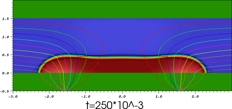
D={(x,y)∈ℝ2:|x|≥32,y=−12}.D=\left\{(x,y)\in\mathbb{R}^{2}:|x|\geq\frac{3}{2},\ y=-\frac{1}{2}\right\}.
Refer to caption
Refer to caption
Refer to caption
Refer to caption
Refer to caption
Refer to caption
Refer to caption
Refer to caption
Refer to caption
Refer to caption
Refer to caption
Refer to caption
Refer to caption
Refer to caption
Refer to caption
Refer to caption
Refer to caption
Refer to caption
Figure 5.2. Splitting of a droplet under the action of an external voltage. The material parameters are ρ1/ρ2=100\rho_{1}/\rho_{2}=100, η1/η2=10\eta_{1}/\eta_{2}=10, γ=50\gamma=50, K1/K2=10K_{1}/K_{2}=10, ε1/ε2=5{\varepsilon}_{1}/{\varepsilon}_{2}=5, εD/ε2=100{\varepsilon}_{D}/{\varepsilon}_{2}=100, M=10−2M=10^{-2}, α=10−3\alpha=10^{-3}, β=10\beta=10, θs=120∘\theta_{s}=120^{\circ}, δ=5⋅10−2\delta=5\cdot 10^{-2}, λ=0.5\lambda=0.5 and V00=20V_{00}=20. The interface is shown at times 00, 0.250.25, 0.50.5, 0.750.75, 1.01.0, 1.251.25, 1.51.5, 1.751.75, 2.02.0, 2.252.25, 2.52.5, 2.752.75, 3.03.0, 3.023.02, 3.053.05, 3.103.10, 3.253.25 and 3.53.5. Colored lines are used to represent the iso-values of the voltage. The black dotted line is the position of the interface at the beginning of the computations.

Figure 5.2 shows the evolution of the system. Notice that, other than adapting the mesh so as to resolve the interfacial layer, nothing else is done and the topological change is handled without the necessity to detect it or to adapt the time-step.

5.3. Merging of Two Droplets

To finalize let us show an example illustrating the merging of two droplets of the same material via electric actuation. The geometrical configuration is the same as in §5.2. In this case, however, there are initially two droplets of heavier material, each one of radius 0.50.5 and centered at (−0.7,0)(-0.7,0) and (0.7,0)(0.7,0), respectively. The material parameters are the same as in §5.2, except the interfacial thickness, which is set to δ=10−2\delta=10^{-2}. We apply an external voltage so that

D={(x,y)∈ℝ2:|x|≤12,y=−12}.D=\left\{(x,y)\in\mathbb{R}^{2}:\ |x|\leq\frac{1}{2},\ y=-\frac{1}{2}\right\}.

To be able to capture the fine interfacial dynamics that merging possesses, we set the initial level of refinement to 44, with 33 extra refinements near the interface, so that the number of cells is 48,69648,696 with a local mesh size away of the interface of about 0.028750.02875 and near the interface of about 6⋅10−36\cdot 10^{-3}. This amounts to a total of 147,249147,249 degrees of freedom. The time-step, again, is set to Δ​t=10−3{\Delta t}=10^{-3}.

Refer to caption
Refer to caption
Refer to caption
Refer to caption
Refer to caption
Refer to caption
Refer to caption
Refer to caption
Refer to caption
Refer to caption
Figure 5.3. Merging of two droplets under the action of an externally applied voltage. The material parameters are ρ1/ρ2=100\rho_{1}/\rho_{2}=100, η1/η2=10\eta_{1}/\eta_{2}=10, γ=50\gamma=50, K1/K2=10K_{1}/K_{2}=10, ε1/ε2=5{\varepsilon}_{1}/{\varepsilon}_{2}=5, εD/ε2=100{\varepsilon}_{D}/{\varepsilon}_{2}=100, M=10−2M=10^{-2}, α=10−3\alpha=10^{-3}, β=10\beta=10, θs=120∘\theta_{s}=120^{\circ}, δ=10−2\delta=10^{-2}, λ=0.5\lambda=0.5 and V00=20V_{00}=20. The interface is shown at times 00, 11, 22, 33, 3.33.3, 3.43.4, 3.53.5, 44, 55 and 5.55.5. Colored lines are used to represent the iso-values of the voltage. The black dotted line is the position of the interface at the beginning of the computations.

Figure 5.3 shows the evolution of the two droplets under the action of the voltage. Again, other than properly resolving the interfacial layer, we did not need to do anything special to handle the topological change.

6. The Semi-Discrete Problem

In §4.2 we showed that the fully discrete problem always has a solution and that, moreover, this solution satisfies certain a priori estimates. Our purpose here is to pass to the limit for h→0h\rightarrow 0 so as to show that a semi-discrete (that is continuous in space and discrete in time) version of our electrowetting model always has a solution.

Let us begin by defining the semi-discrete problem. Given initial data and an external voltage, we find:

{VΔ​t−V¯0,Δ​t,qΔ​t,ϕΔ​t,μΔ​t,𝐮Δ​t,pΔ​t}⊂H⋆1(Ω⋆)×H1(Ω)3×𝐕×L∫=02(Ω)\left\{V_{{\Delta t}}-\bar{V}_{0,{\Delta t}},q_{{\Delta t}},\phi_{{\Delta t}},\mu_{{\Delta t}},{\bf u}_{{\Delta t}},p_{{\Delta t}}\right\}\subset H^{1}_{\star}(\Omega^{\star})\times{{H}^{1}(\Omega)}^{3}\times{\bf V}\times{L^{2}_{\scriptscriptstyle\!\int\!=0}(\Omega)}

that solve:

Initialization:

For n=0n=0, let q0q^{0}, ϕ0\phi^{0} and 𝐮0{\bf u}^{0} equal the initial charge, phase field and velocity, respectively.

Time Marching:

For 0≤n≤N−10\leq n\leq N-1 we compute

(Vn+1,qn+1,ϕn+1,μn+1,𝐮n+1,pn+1)∈H⋆1(Ω⋆)+V¯0n+1×H1(Ω)3×𝐕×L∫=02(Ω),(V^{n+1},q^{n+1},\phi^{n+1},\mu^{n+1},{\bf u}^{n+1},p^{n+1})\in H^{1}_{\star}(\Omega^{\star})+\bar{V}_{0}^{n+1}\times{{H}^{1}(\Omega)}^{3}\times{\bf V}\times{L^{2}_{\scriptscriptstyle\!\int\!=0}(\Omega)},

that solve:

(6.1) ⟨ε⋆(ϕn+1)∇Vn+1,∇W⟩Ω⋆=⟨qn+1,W⟩,∀W∈H01(Ω⋆),\left\langle{\varepsilon}^{\star}(\phi^{n+1})\nabla V^{n+1},\nabla W\right\rangle_{\Omega^{\star}}=\left\langle q^{n+1},W\right\rangle,\quad\forall W\in H^{1}_{0}(\Omega^{\star}),
(6.2) ⟨𝔡​qn+1Δ​t,r⟩−⟨qn𝐮n+1,∇r⟩+⟨K(ϕn)∇(λqn+1+Vn+1),∇r⟩=0,∀r∈H1(Ω)\left\langle\frac{{\mathfrak{d}}q^{n+1}}{{\Delta t}},r\right\rangle-\left\langle q^{n}{\bf u}^{n+1},\nabla r\right\rangle+\left\langle K(\phi^{n})\nabla\left(\lambda q^{n+1}+V^{n+1}\right),\nabla r\right\rangle=0,\quad\forall r\in{{H}^{1}(\Omega)}
(6.3) ⟨𝔡​ϕn+1Δ​t,ϕ¯⟩+⟨𝐮n+1⋅∇ϕn,ϕ¯⟩+⟨M(ϕn)∇μn+1,∇ϕ¯⟩=0,∀ϕ¯∈H1(Ω)\left\langle\frac{{\mathfrak{d}}\phi^{n+1}}{{\Delta t}},\bar{\phi}\right\rangle+\left\langle{\bf u}^{n+1}{\cdot}\nabla\phi^{n},\bar{\phi}\right\rangle+\left\langle M(\phi^{n})\nabla\mu^{n+1},\nabla\bar{\phi}\right\rangle=0,\quad\forall\bar{\phi}\in{{H}^{1}(\Omega)}
(6.4) ⟨μn+1,μ¯⟩=γδ​⟨𝒲′​(ϕn)+𝒜​𝔡​ϕn+1,μ¯⟩+γ​δ​⟨∇ϕn+1,∇μ¯⟩+12​⟨ρ′​(ϕn)​𝐮n⋅𝐮n+1,μ¯⟩−12​⟨ℰ⁡(ϕn+1,ϕn)​|∇Vn+1|2,μ¯⟩+α⁡[𝔡​ϕn+1Δ​t+𝐮𝝉n+1​ψ​(ϕn),μ¯]+γ⁡[Θf​s′​(ϕn)+ℬ​𝔡​ϕn+1,μ¯]∀μ¯∈H1​(Ω)∩L∞​(Ω),\left\langle\mu^{n+1},\bar{\mu}\right\rangle=\frac{\gamma}{\delta}\left\langle{\mathcal{W}}^{\prime}(\phi^{n})+{\mathcal{A}}{\mathfrak{d}}\phi^{n+1},\bar{\mu}\right\rangle+\gamma\delta\left\langle\nabla\phi^{n+1},\nabla\bar{\mu}\right\rangle+\frac{1}{2}\left\langle\rho^{\prime}(\phi^{n}){\bf u}^{n}{\cdot}{\bf u}^{n+1},\bar{\mu}\right\rangle\\ -\frac{1}{2}\left\langle{\mathcal{E}}(\phi^{n+1},\phi^{n})|\nabla V^{n+1}|^{2},\bar{\mu}\right\rangle+\alpha\left[\frac{{\mathfrak{d}}\phi^{n+1}}{{\Delta t}}+{\bf u}_{\boldsymbol{\tau}}^{n+1}\psi(\phi^{n}),\bar{\mu}\right]\\ +\gamma\left[\Theta_{fs}^{\prime}(\phi^{n})+{\mathcal{B}}{\mathfrak{d}}\phi^{n+1},\bar{\mu}\right]\quad\forall\bar{\mu}\in{{H}^{1}(\Omega)}\cap L^{\infty}(\Omega),
(6.5a) ⟨ρ⁡(ϕn+1)¯​𝐮n+1−ρ⁡(ϕn)​𝐮nΔ​t,𝐰⟩+⟨ρ(ϕn)𝐮n⋅∇𝐮n+1+12∇⋅(ρ(ϕn)𝐮n)𝐮n+1,𝐰⟩+⟨η⁡(ϕn)​𝐒​(𝐮n+1),𝐒⁡(𝐰)⟩−⟨pn+1,∇⋅𝐰⟩+[β⁡(ϕn)​𝐮𝝉n+1,𝐰𝝉]+α⁡[𝐮𝝉n+1​ψ​(ϕn),𝐰𝝉​ψ​(ϕn)]=⟨μn+1∇ϕn,𝐰⟩−⟨qn∇(λqn+1+Vn+1),𝐰⟩+12⟨ρ′(ϕn)𝔡​ϕn+1Δ​t𝐮n,𝐰⟩−α⁡[𝔡​ϕn+1Δ​t,𝐰𝝉​ψ​(ϕn)],∀𝐰∈𝐕,\left\langle\frac{\overline{\rho(\phi^{n+1})}{\bf u}^{n+1}-\rho(\phi^{n}){\bf u}^{n}}{{\Delta t}},{\bf w}\right\rangle+\left\langle\rho(\phi^{n}){\bf u}^{n}{\cdot}\nabla{\bf u}^{n+1}+\frac{1}{2}\nabla\!{\cdot}(\rho(\phi^{n}){\bf u}^{n}){\bf u}^{n+1},{\bf w}\right\rangle\\ +\left\langle\eta(\phi^{n}){\bf S}({\bf u}^{n+1}),{\bf S}({\bf w})\right\rangle-\left\langle p^{n+1},\nabla\!{\cdot}{\bf w}\right\rangle+\left[\beta(\phi^{n}){\bf u}_{{\boldsymbol{\tau}}}^{n+1},{\bf w}_{{\boldsymbol{\tau}}}\right]+\alpha\left[{\bf u}_{{\boldsymbol{\tau}}}^{n+1}\psi(\phi^{n}),{\bf w}_{{\boldsymbol{\tau}}}\psi(\phi^{n})\right]\\ =\left\langle\mu^{n+1}\nabla\phi^{n},{\bf w}\right\rangle-\left\langle q^{n}\nabla(\lambda q^{n+1}+V^{n+1}),{\bf w}\right\rangle+\frac{1}{2}\left\langle\rho^{\prime}(\phi^{n})\frac{{\mathfrak{d}}\phi^{n+1}}{{\Delta t}}{\bf u}^{n},{\bf w}\right\rangle\\ -\alpha\left[\frac{{\mathfrak{d}}\phi^{n+1}}{{\Delta t}},{\bf w}_{{\boldsymbol{\tau}}}\psi(\phi^{n})\right],\quad\forall{\bf w}\in{\bf V},
(6.5b) ⟨p¯,∇⋅𝐮n+1⟩=0,∀p¯∈L∫=02(Ω).\left\langle\bar{p},\nabla\!{\cdot}{\bf u}^{n+1}\right\rangle=0,\quad\forall\bar{p}\in{L^{2}_{\scriptscriptstyle\!\int\!=0}(\Omega)}.
Remark 6.6 (Permittivity).

Notice that, in our definition of solution, the test function for equation (6.4) needs to be bounded. This is necessary to make sense of the term

⟨ℰ⁡(ϕn+1,ϕn)​|∇Vn+1|2,μ¯⟩,\left\langle{\mathcal{E}}(\phi^{n+1},\phi^{n})|\nabla V^{n+1}|^{2},\bar{\mu}\right\rangle,

since ℰ{\mathcal{E}} is bounded by construction and Vn+1∈H1​(Ω)V^{n+1}\in{{H}^{1}(\Omega)}. The authors of [20] used a similar choice of test functions and showed, using different techniques, existence of a solution for their model of electrowetting in the case when the permittivity is phase-dependent.

Since the solution to the fully discrete problem (4.4)–(4.9) exists for all values of h>0h>0 and satisfies uniform bounds, one expects the sequence of discrete solutions to converge, in some topology, and that the limit is a solution of problem (6.1)–(6.5). The following result shows that this is indeed the case.

Theorem 6.7 (Existence and stability).

For all Δ​t>0{\Delta t}>0, problem (6.1)–(6.5) has a solution. Moreover, this solution satisfies an energy estimate, analogous to (4.16), where the constant cc might depend on Δ​t{\Delta t} and the data of the problem, but not on the solution.

Proof.

Theorem 4.21 shows the existence, for every h>0h>0, of a solution to the fully discrete problem (4.4)–(4.9) which, moreover, satisfies estimate (4.16). This estimate implies that, for every nn, as h→0h\rightarrow 0:

  • •

    𝒲⁡(ϕhn){\mathcal{W}}(\phi_{h}^{n}) remains bounded in L1​(Ω)L^{1}(\Omega). Since the modified Ginzburg-Landau potential is a quadratic function of its argument, this implies that there is a subsequence, labeled again ϕhn\phi_{h}^{n}, that converges weakly in L2​(Ω){{L}^{2}(\Omega)}.

  • •

    ∇ϕhn\nabla\phi_{h}^{n} remains bounded in 𝐋2{\bf L}^{2}. This, together with the previous observation, gives us a subsequence that converges weakly in H1​(Ω){{H}^{1}(\Omega)} and strongly in L2​(Ω){{L}^{2}(\Omega)}.

  • •

    The strong L2L^{2}-convergence of ϕhn\phi_{h}^{n} implies that the convergence is almost everywhere and, since all the material functions are assumed continuous, the coefficients converge also almost everywhere.

  • •

    There is a subsequence of 𝐮hn+1{\bf u}_{h}^{n+1} that converges weakly in 𝐕{\bf V} and strongly in 𝐋2​(Ω){{\bf L}^{2}(\Omega)}.

  • •

    A subsequence of Vhn−V¯0nV_{h}^{n}-\bar{V}_{0}^{n} converges weakly in H⋆1​(Ω⋆)H^{1}_{\star}(\Omega^{\star}) and hence strongly in L2​(Ω⋆)L^{2}(\Omega^{\star}).

  • •

    There is a subsequence of qhn+1q_{h}^{n+1} that converges weakly in L2​(Ω){{L}^{2}(\Omega)}. Moreover, we know that K(ϕhn)∇(λqhn+1+Vhn+1)K(\phi_{h}^{n})\nabla(\lambda q_{h}^{n+1}+V_{h}^{n+1}) converges weakly. By the a.e. convergence of the coefficients and the L2L^{2}-weak convergence of ∇Vhn+1\nabla V_{h}^{n+1} we conclude that ∇qhn+1\nabla q_{h}^{n+1} must converge weakly and, thus, the convergence is weak in H1​(Ω){{H}^{1}(\Omega)} and strong in L2​(Ω){{L}^{2}(\Omega)}.

  • •

    The quantity ϕ˙hn+1=𝔡​ϕhn+1Δ​t+𝐮h​𝝉n+1​ψ​(ϕhn)\dot{\phi}_{h}^{n+1}=\tfrac{{\mathfrak{d}}\phi_{h}^{n+1}}{{\Delta t}}+{\bf u}_{h{\boldsymbol{\tau}}}^{n+1}\psi(\phi_{h}^{n}) remains bounded in L2​(Γ)L^{2}(\Gamma), which implies that there is a subsequence of ϕ˙hn+1\dot{\phi}_{h}^{n+1} that converges weakly in L2​(Γ)L^{2}(\Gamma).

  • •

    ∇μhn\nabla\mu_{h}^{n} remains bounded in 𝐋2​(Ω){{\bf L}^{2}(\Omega)}. Moreover, setting μ¯h=1\bar{\mu}_{h}=1 in (4.7) and the observations given above, imply

    |⟨μhn+1,1⟩|≤|γδ⟨𝒲′(ϕhk)+𝒜𝔡ϕhk+1,1⟩+12⟨ρ′(ϕhn)𝐮hn,𝐮hn+1⟩+α[ϕ˙hk+1,1]+γ[Θf​s′(ϕhn)+ℬ𝔡ϕhn+1,1]|≤c,\left|\left\langle\mu_{h}^{n+1},1\right\rangle\right|\leq\left|\frac{\gamma}{\delta}\left\langle{\mathcal{W}}^{\prime}(\phi_{h}^{k})+{\mathcal{A}}{\mathfrak{d}}\phi_{h}^{k+1},1\right\rangle\right.\\ \left.+\frac{1}{2}\left\langle\rho^{\prime}(\phi_{h}^{n}){\bf u}_{h}^{n},{\bf u}_{h}^{n+1}\right\rangle+\alpha\left[\dot{\phi}_{h}^{k+1},1\right]+\gamma\left[\Theta_{fs}^{\prime}(\phi_{h}^{n})+{\mathcal{B}}{\mathfrak{d}}\phi_{h}^{n+1},1\right]\right|\leq c,

    which shows that ∫Ωμhn+1\int_{\Omega}\mu_{h}^{n+1} remains bounded and, thus, μhn\mu_{h}^{n} remains bounded in H1​(Ω){{H}^{1}(\Omega)} and so there is a subsequence that converges weakly in H1​(Ω){{H}^{1}(\Omega)} and strongly in L2​(Ω){{L}^{2}(\Omega)}.

  • •

    Finally, we use the compatibility condition (4.2) and the discrete momentum equation (4.9a) to obtain an estimate on the pressure phn+1p_{h}^{n+1},

    c​‖phn+1‖L2≤1Δ​t​‖ρ⁡(ϕhn)‖L∞​‖𝔡​𝐮hn+1‖𝐋2+1Δ​t​‖𝔡​ρ​(ϕhn+1)‖L∞​‖𝐮hn+1‖𝐋2+‖ρ⁡(ϕhn)‖L∞​‖𝐮hn‖𝐇1​‖𝐮hn+1‖𝐇1+‖ρ′​(ϕhn)‖L∞​‖∇ϕhn‖𝐋2​‖𝐮hn‖𝐇1​‖𝐮hn+1‖𝐇1+‖η⁡(ϕhn)‖L∞​‖𝐒⁡(𝐮hn+1)‖𝐋2+‖β⁡(ϕhn)‖L∞​‖𝐮hn+1‖𝐕+α​‖ψ⁡(ϕhn)‖L∞​(Γ)​‖ϕ˙hn+1‖L2​(Γ)+‖μhn+1‖H1​‖∇ϕhn‖𝐋2+‖qhn+1‖H1​‖∇(λ​qhn+1+Vhn+1)‖𝐋2+1Δ​t​‖ρ′​(ϕhn)‖L∞​‖𝔡​ϕhn+1‖L2​‖𝐮hn‖𝐕≤cΔ​t,c\|p^{n+1}_{h}\|_{L^{2}}\leq\frac{1}{{\Delta t}}\|\rho(\phi_{h}^{n})\|_{L^{\infty}}\|{\mathfrak{d}}{\bf u}_{h}^{n+1}\|_{{\bf L}^{2}}+\frac{1}{{\Delta t}}\|{\mathfrak{d}}\rho(\phi_{h}^{n+1})\|_{L^{\infty}}\|{\bf u}_{h}^{n+1}\|_{{\bf L}^{2}}+\|\rho(\phi_{h}^{n})\|_{L^{\infty}}\|{\bf u}_{h}^{n}\|_{{\bf H}^{1}}\|{\bf u}_{h}^{n+1}\|_{{\bf H}^{1}}\\ +\|\rho^{\prime}(\phi_{h}^{n})\|_{L^{\infty}}\|\nabla\phi_{h}^{n}\|_{{\bf L}^{2}}\|{\bf u}_{h}^{n}\|_{{\bf H}^{1}}\|{\bf u}_{h}^{n+1}\|_{{\bf H}^{1}}+\|\eta(\phi_{h}^{n})\|_{L^{\infty}}\|{\bf S}({\bf u}_{h}^{n+1})\|_{{\bf L}^{2}}+\|\beta(\phi_{h}^{n})\|_{L^{\infty}}\|{\bf u}_{h}^{n+1}\|_{{\bf V}}\\ +\alpha\|\psi(\phi_{h}^{n})\|_{L^{\infty}(\Gamma)}\|\dot{\phi}_{h}^{n+1}\|_{L^{2}(\Gamma)}+\|\mu_{h}^{n+1}\|_{H^{1}}\|\nabla\phi_{h}^{n}\|_{{\bf L}^{2}}+\|q_{h}^{n+1}\|_{H^{1}}\|\nabla(\lambda q_{h}^{n+1}+V_{h}^{n+1})\|_{{\bf L}^{2}}\\ +\frac{1}{{\Delta t}}\|\rho^{\prime}(\phi_{h}^{n})\|_{L^{\infty}}\|{\mathfrak{d}}\phi_{h}^{n+1}\|_{L^{2}}\|{\bf u}_{h}^{n}\|_{{\bf V}}\leq\frac{c}{{\Delta t}},

    which, for a fixed and positive Δ​t{\Delta t}, implies the existence of a L2L^{2}-weakly convergent subsequence.

Let us denote the limit by

{VΔ​t−V¯0,Δ​t,qΔ​t,ϕΔ​t,μΔ​t,𝐮Δ​t,pΔ​t}⊂H⋆1(Ω⋆)×H1(Ω)3×𝐕×L∫=02(Ω).\left\{V_{{\Delta t}}-\bar{V}_{0,{\Delta t}},q_{{\Delta t}},\phi_{{\Delta t}},\mu_{{\Delta t}},{\bf u}_{{\Delta t}},p_{{\Delta t}}\right\}\subset H^{1}_{\star}(\Omega^{\star})\times{{H}^{1}(\Omega)}^{3}\times{\bf V}\times{L^{2}_{\scriptscriptstyle\!\int\!=0}(\Omega)}.

It remains to show that this limit is a solution of (6.1)–(6.5):

Equation (6.1):

Notice that if we show that, as h→0h\rightarrow 0, the sequence Vhn+1V_{h}^{n+1} converges to Vn+1V^{n+1} strongly in H⋆1​(Ω⋆)H^{1}_{\star}(\Omega^{\star}), then the a.e. convergence of the coefficients implies

(6.8) ⟨ε⋆(ϕhn+1)∇Vhn+1,∇W⟩Ω⋆→⟨ε⋆(ϕn+1)∇Vn+1,∇W⟩Ω⋆.\left\langle{\varepsilon}^{\star}(\phi_{h}^{n+1})\nabla V_{h}^{n+1},\nabla W\right\rangle_{\Omega^{\star}}\rightarrow\left\langle{\varepsilon}^{\star}(\phi^{n+1})\nabla V^{n+1},\nabla W\right\rangle_{\Omega^{\star}}.

Let us then show the strong convergence by an argument similar to that of [20, pp. 2778]. For any function V∈H⋆1​(Ω⋆),V\in H^{1}_{\star}(\Omega^{\star}), we introduce the elliptic projection 𝒫h​V∈𝕎h​(V){\mathcal{P}}_{h}V\in{\mathbb{W}}_{h}(V) as the solution to

⟨∇𝒫hV,∇Wh⟩Ω⋆=⟨∇V,∇Wh⟩Ω⋆,∀Wh∈𝕎h(0).\left\langle\nabla{\mathcal{P}}_{h}V,\nabla W_{h}\right\rangle_{\Omega^{\star}}=\left\langle\nabla V,\nabla W_{h}\right\rangle_{\Omega^{\star}},\quad\forall W_{h}\in{\mathbb{W}}_{h}(0).

It is well known that 𝒫h​V→V{\mathcal{P}}_{h}V\rightarrow V strongly in H⋆1​(Ω⋆)H^{1}_{\star}(\Omega^{\star}). Given that ε{\varepsilon} is uniformly bounded,

c​‖∇(Vhn+1−Vn+1)‖𝐋22\displaystyle c\|\nabla(V_{h}^{n+1}-V^{n+1})\|_{{\bf L}^{2}}^{2} ≤⟨ε⋆(ϕhn+1)∇(Vhn+1−Vn+1),∇(Vhn+1−Vn+1)⟩Ω⋆\displaystyle\leq\left\langle{\varepsilon}^{\star}(\phi_{h}^{n+1})\nabla(V_{h}^{n+1}-V^{n+1}),\nabla(V_{h}^{n+1}-V^{n+1})\right\rangle_{\Omega^{\star}}
=⟨ε⋆(ϕhn+1)∇Vhn+1,∇(𝒫hVn+1−Vn+1)⟩Ω⋆\displaystyle=\left\langle{\varepsilon}^{\star}(\phi_{h}^{n+1})\nabla V_{h}^{n+1},\nabla({\mathcal{P}}_{h}V^{n+1}-V^{n+1})\right\rangle_{\Omega^{\star}}
+⟨ε⋆(ϕhn+1)∇Vhn+1,∇(Vhn+1−𝒫hVn+1)⟩Ω⋆\displaystyle+\left\langle{\varepsilon}^{\star}(\phi_{h}^{n+1})\nabla V_{h}^{n+1},\nabla(V_{h}^{n+1}-{\mathcal{P}}_{h}V^{n+1})\right\rangle_{\Omega^{\star}}
+⟨ε⋆(ϕhn+1)∇Vn+1,∇(Vn+1−Vhn+1)⟩Ω⋆\displaystyle+\left\langle{\varepsilon}^{\star}(\phi_{h}^{n+1})\nabla V^{n+1},\nabla(V^{n+1}-V_{h}^{n+1})\right\rangle_{\Omega^{\star}}
=I+I​I+I​I​I.\displaystyle=I+II+III.

Let us estimate each one of the terms separately. Since the coefficients are bounded and the sequence ∇Vhn+1\nabla V_{h}^{n+1} is uniformly bounded in 𝐋2​(Ω){{\bf L}^{2}(\Omega)}, the strong convergence of 𝒫h​Vn+1{\mathcal{P}}_{h}V^{n+1} shows that I→0I\rightarrow 0. For I​III we use the equation, namely

II=⟨ε⋆(ϕhn+1)∇Vhn+1,∇(Vhn+1−𝒫hVn+1)⟩Ω⋆=⟨qhn+1,Vhn+1−𝒫hVn+1⟩→0II=\left\langle{\varepsilon}^{\star}(\phi_{h}^{n+1})\nabla V_{h}^{n+1},\nabla(V_{h}^{n+1}-{\mathcal{P}}_{h}V^{n+1})\right\rangle_{\Omega^{\star}}=\left\langle q_{h}^{n+1},V_{h}^{n+1}-{\mathcal{P}}_{h}V^{n+1}\right\rangle\rightarrow 0

since qhn+1q_{h}^{n+1} converges strongly in L2​(Ω){{L}^{2}(\Omega)}. Finally, notice that the last term can be rewritten as

I​I​I\displaystyle III =⟨(ε⋆(ϕhn+1)⟧−ε⋆(ϕn+1)∇Vn+1,∇(Vn+1−Vhn+1)⟩Ω⋆\displaystyle=\left\langle\left({\varepsilon}^{\star}(\phi_{h}^{n+1})\rrbracket-{\varepsilon}^{\star}(\phi^{n+1}\right)\nabla V^{n+1},\nabla(V^{n+1}-V_{h}^{n+1})\right\rangle_{\Omega^{\star}}
+⟨ε⋆(ϕn+1)∇Vn+1,∇(Vn+1−Vhn+1)⟩Ω⋆\displaystyle+\left\langle{\varepsilon}^{\star}(\phi^{n+1})\nabla V^{n+1},\nabla(V^{n+1}-V_{h}^{n+1})\right\rangle_{\Omega^{\star}}

The uniform boundedness of ∇Vhn+1\nabla V_{h}^{n+1} in 𝐋2​(Ω){{\bf L}^{2}(\Omega)} implies that, for the first term, it suffices to show that (ε⋆(ϕhn+1)−ε⋆(ϕn+1))∇Vn+1→0\left({\varepsilon}^{\star}(\phi_{h}^{n+1})-{\varepsilon}^{\star}(\phi^{n+1})\right)\nabla V^{n+1}\rightarrow 0 in 𝐋2​(Ω){{\bf L}^{2}(\Omega)}, which follows from the Lebesgue dominated convergence theorem. For the second term, use the weak convergence of ∇Vhn+1\nabla V_{h}^{n+1}. This, together with the strong L2L^{2}-convergence of qhn+1q_{h}^{n+1} implies that the limit solves (6.1).

Equation (6.2):

The strong L2L^{2}-convergence of qhn+1q_{h}^{n+1} implies that 1Δ​t​𝔡​qhn+1→1Δ​t​𝔡​qn+1\tfrac{1}{{\Delta t}}{\mathfrak{d}}q_{h}^{n+1}\rightarrow\tfrac{1}{{\Delta t}}{\mathfrak{d}}q^{n+1} strongly in L2​(Ω){{L}^{2}(\Omega)}. Using the compact embeddings H1​(Ω)⋐L4​(Ω){{H}^{1}(\Omega)}\Subset L^{4}(\Omega) and 𝐕⋐𝐋4​(Ω){\bf V}\Subset{\bf L}^{4}(\Omega), we see that

⟨qhn​𝐮hn+1,∇r⟩→⟨qn​𝐮n+1,∇r⟩,∀r∈H1​(Ω),\left\langle q_{h}^{n}{\bf u}_{h}^{n+1},\nabla r\right\rangle\rightarrow\left\langle q^{n}{\bf u}^{n+1},\nabla r\right\rangle,\quad\forall r\in{{H}^{1}(\Omega)},

as h→0h\rightarrow 0. The term K(ϕhn)∇(λqhn+1+Vhn+1)K(\phi_{h}^{n})\nabla(\lambda q_{h}^{n+1}+V_{h}^{n+1}) can be treated as in (6.8). These observations imply that the limit solves (6.2).

Equation (6.3):

The strong 𝐋2{\bf L}^{2}-convergence of 𝐮hn+1{\bf u}_{h}^{n+1}, the weak H1H^{1}-convergence of ϕhn+1\phi_{h}^{n+1} and an argument similar to (6.8) imply that the limit solves (6.3).

Equation (6.4):

The smoothness of 𝒲{\mathcal{W}} and the fact its growth is quadratic imply

|⟨𝒲′​(ϕhn)−𝒲′​(ϕn),μ¯⟩|≤maxφ⁡|𝒲′′​(φ)|​‖ϕhn−ϕn‖L2​‖μ¯‖L2→0.\left|\left\langle{\mathcal{W}}^{\prime}(\phi_{h}^{n})-{\mathcal{W}}^{\prime}(\phi^{n}),\bar{\mu}\right\rangle\right|\leq\max_{\varphi}|{\mathcal{W}}^{\prime\prime}(\varphi)|\|\phi_{h}^{n}-\phi^{n}\|_{L^{2}}\|\bar{\mu}\|_{L^{2}}\rightarrow 0.

A similar argument and the embedding H1​(Ω)⋐L2​(Γ){{H}^{1}(\Omega)}\Subset L^{2}(\Gamma) can be used to show convergence of Θf​s′​(ϕhn)\Theta_{fs}^{\prime}(\phi_{h}^{n}). Since ρ\rho is a bounded smooth function,

⟨ρ′​(ϕhn)​𝐮hn⋅𝐮hn+1,μ¯⟩→⟨ρ′​(ϕn)​𝐮n⋅𝐮n+1,μ¯⟩.\left\langle\rho^{\prime}(\phi_{h}^{n}){\bf u}_{h}^{n}{\cdot}{\bf u}_{h}^{n+1},\bar{\mu}\right\rangle\rightarrow\left\langle\rho^{\prime}(\phi^{n}){\bf u}^{n}{\cdot}{\bf u}^{n+1},\bar{\mu}\right\rangle.

The strong 𝐋2{\bf L}^{2}-convergence of ∇Vhn+1\nabla V_{h}^{n+1} implies that

⟨ℰ⁡(ϕhn+1,ϕhn)​|∇Vhn+1|2,μ¯⟩→⟨ℰ⁡(ϕn+1,ϕn)​|∇Vn+1|2,μ¯⟩,\left\langle{\mathcal{E}}(\phi_{h}^{n+1},\phi_{h}^{n})|\nabla V_{h}^{n+1}|^{2},\bar{\mu}\right\rangle\rightarrow\left\langle{\mathcal{E}}(\phi^{n+1},\phi^{n})|\nabla V^{n+1}|^{2},\bar{\mu}\right\rangle,

where it is necessary to have μ¯∈L∞​(Ω)\bar{\mu}\in L^{\infty}(\Omega). To conclude that (6.4) is satisfied by the limit, it is left to show that ϕ˙hn+1\dot{\phi}_{h}^{n+1} converges strongly in L2​(Γ)L^{2}(\Gamma). We know that ϕ˙hn+1\dot{\phi}_{h}^{n+1} converges weakly in L2​(Γ)L^{2}(\Gamma). On the other hand 1Δ​t​𝔡​ϕhn+1\tfrac{1}{{\Delta t}}{\mathfrak{d}}\phi_{h}^{n+1} converges strongly in L2​(Γ)L^{2}(\Gamma), 𝐮h​𝝉n+1{\bf u}_{h{\boldsymbol{\tau}}}^{n+1} converges strongly in 𝐋2​(Γ){\bf L}^{2}(\Gamma) and ψ⁡(ϕhn)\psi(\phi_{h}^{n}) converges a.e. in Γ\Gamma.

Equations (6.5):

Clearly, (6.5b) is satisfied. To show that (6.5a) holds, notice that

⟨ρ⁡(ϕhn+1)¯​𝐮hn+1−ρ⁡(ϕn+1)¯​𝐮n+1,𝐰⟩=⟨ρ⁡(ϕhn+1)¯​(𝐮hn+1−𝐮n+1),𝐰⟩+⟨(ρ⁡(ϕhn+1)¯−ρ⁡(ϕn+1)¯)​𝐮n+1,𝐰⟩→0.\left\langle\overline{\rho(\phi_{h}^{n+1})}{\bf u}_{h}^{n+1}-\overline{\rho(\phi^{n+1})}{\bf u}^{n+1},{\bf w}\right\rangle=\\ \left\langle\overline{\rho(\phi_{h}^{n+1})}\left({\bf u}_{h}^{n+1}-{\bf u}^{n+1}\right),{\bf w}\right\rangle+\left\langle\left(\overline{\rho(\phi_{h}^{n+1})}-\overline{\rho(\phi^{n+1})}\right){\bf u}^{n+1},{\bf w}\right\rangle\rightarrow 0.

Since we assume that ψ\psi is smooth and the slip coefficient β\beta is smooth and depends only on the phase field, but not on the stress (as opposed to §2.4), we can get convergence of the terms [β⁡(ϕhn)​𝐮h​𝝉n+1,𝐰𝝉]\left[\beta(\phi_{h}^{n}){\bf u}_{h{\boldsymbol{\tau}}}^{n+1},{\bf w}_{{\boldsymbol{\tau}}}\right] and [𝐮h​𝝉n+1​ψ​(ϕhn),𝐰𝝉​ψ​(ϕhn)]\left[{\bf u}_{h{\boldsymbol{\tau}}}^{n+1}\psi(\phi_{h}^{n}),{\bf w}_{\boldsymbol{\tau}}\psi(\phi_{h}^{n})\right], respectively. The advection term can be treated using standard arguments and thus we will not give details here. The terms

⟨μhn+1∇ϕhn,𝐰⟩,⟨qhn∇(λqhn+1+Vhn+1),∇𝐰⟩,\left\langle\mu_{h}^{n+1}\nabla\phi_{h}^{n},{\bf w}\right\rangle,\qquad\left\langle q_{h}^{n}\nabla(\lambda q_{h}^{n+1}+V_{h}^{n+1}),\nabla{\bf w}\right\rangle,

can be treated using arguments similar to the ones given before. The term

⟨ρ′​(ϕhn)​𝔡​ϕhn+1Δ​t​𝐮hn,𝐰⟩,\left\langle\rho^{\prime}(\phi_{h}^{n})\frac{{\mathfrak{d}}\phi_{h}^{n+1}}{{\Delta t}}{\bf u}_{h}^{n},{\bf w}\right\rangle,

can be easily shown to converge since all terms converge strongly. The convergence of the term

[𝔡​ϕhn+1Δ​t,𝐰𝝉​ψ​(ϕhn)],\left[\frac{{\mathfrak{d}}\phi_{h}^{n+1}}{{\Delta t}},{\bf w}_{{\boldsymbol{\tau}}}\psi(\phi_{h}^{n})\right],

follows again from the compact embedding H1​(Ω)⋐L2​(Γ){{H}^{1}(\Omega)}\Subset L^{2}(\Gamma). Finally, the convergence of the viscous stress term follows the lines of the proof of (6.8).

To conlcude, we notice that we do not need to reprove estimates similar to (4.16). These are uniformly valid, in hh, for all terms in the sequence and, therefore, valid for the limit. Moreover, if one wanted to obtain an energy estimate by repeating the arguments used to obtain Proposition 4.14 it would be necessary first to obtain uniform L∞L^{\infty} bounds on the sequence 𝔡​ϕh,Δ​t{\mathfrak{d}}\phi_{h,{\Delta t}}, since one of the steps in the proof requires setting μ¯h=2​𝔡​ϕhn+1\bar{\mu}_{h}=2{\mathfrak{d}}\phi_{h}^{n+1}. ∎

Remark 6.9 (Limit Δ​t→0{\Delta t}\rightarrow 0).

We are not able to pass to the limit when Δ​t→0{\Delta t}\rightarrow 0 for several reasons. First, the estimates on the pressure depend on the time-step and getting around this would require finer estimates on the time derivative of the velocity, this is standard for Navier Stokes. In addition, the terms

⟨ρ′​(ϕn)​𝔡​ϕn+1Δ​t​𝐮n,𝐰⟩,⟨𝔡​ρ​(ϕn+1)Δ​t​𝐮n+1,𝐰⟩,\left\langle\rho^{\prime}(\phi^{n})\frac{{\mathfrak{d}}\phi^{n+1}}{{\Delta t}}{\bf u}^{n},{\bf w}\right\rangle,\qquad\left\langle\frac{{\mathfrak{d}}\rho(\phi^{n+1})}{{\Delta t}}{\bf u}^{n+1},{\bf w}\right\rangle,

would require finer estimates on the time derivative of the phase field which we have not been able to show. It might be possible, however, to circumvent these two restrictions by defining the weak solution to the continuous problem with an unconstrained formulation for the momentum equation (i.e., solution and test functions in 𝐕{\bf V}) and modifying the Cahn-Hilliard equations to their “viscous version”, in other words suitably adding a term of the form ϕt\phi_{t}. We will not pursue this direction.

7. Conclusions and Perspectives

Some possible directions for future work would be to extend the analysis by passing to the limit as Δ​t→0{\Delta t}\rightarrow 0, or investigate the phenomenological pinning model more thoroughly. It would also be interesting to look at the use of open boundary conditions on ∂⋆Ω⋆\partial^{\star}\Omega^{\star}, which is more physically correct for some electrowetting devices. As far as we know, this is an open area of research in the context of phase-field methods. Other extensions of the model could include the transport of surfactant at the liquid-gas interface, though this would make the model more complicated. We want to emphasize that our model gives physically reasonable results when modeling actual electrowetting systems, and so could be used within an optimization framework for improving device design.

Concerning numerics, an important issue that has not been addressed is how to actually solve the discretized systems. Even in the fully uncoupled case, the pressence of the dynamic boundary condition in the Cahn-Hilliard system (Step 2 in the scheme of section 5) makes this problem extremely ill-conditioned and standard preconditioning techniques (for instance the one in [8]) inapplicable.

References

  • [1] H. Abels, H. Garcke, and G. Grün. Thermodynamically consistent diffuse interface models for incompressible two-phase flows with different densities. Math. Mod. Meths. Appli. Sci. (M3AS), 2011. To appear.
  • [2] R.A. Adams and J.J.F. Fournier. Sobolev spaces. 2nd ed. Pure and Applied Mathematics 140. New York, NY: Academic Press. xiii, 305 p., 2003.
  • [3] H. Aminfar and M. Mohammadpourfard. Lattice Boltzmann method for electrowetting modeling and simulation. Comput. Methods Appl. Mech. Engrg., 198(47-48):3852–3868, 2009.
  • [4] H. Aminfar and M. Mohammadpourfard. Lattice Boltzmann simulation of droplet base electrowetting. Int. J. Comput. Fluid Dyn., 24(5):143–156, 2010.
  • [5] D. Aronov, M. Molotskii, and G. Rosenman. Electron-induced wettability modification. Phys. Rev. B, 76:035437, Jul 2007.
  • [6] W. Bangerth, R. Hartmann, and G. Kanschat. deal.II Differential Equations Analysis Library, Technical Reference. http://www.dealii.org.
  • [7] W. Bangerth, R. Hartmann, and G. Kanschat. deal.II — a general-purpose object-oriented finite element library. ACM Trans. Math. Softw., 33(4), 2007.
  • [8] E. Bänsch, P Morin, and R.H. Nochetto. Preconditioning a class of fourth order problems by operator splitting. Numer. Math., 118(2):197–228, 2011.
  • [9] B. Berge. Électrocapillarité et mouillage de films isolants par l’eau (including an english translation). Comptes Rendus de l’Académie des Sciences de Paris, Série II, 317:157–163, 1993.
  • [10] B. Berge and J. Peseux. Variable focal lens controlled by an external voltage: An application of electrowetting. European Physical Journal E, 3(2):159–163, 2000.
  • [11] F. Brezzi and M. Fortin. Mixed and Hybrid Finite Element Methods. Springer-Verlag, New York, NY, 1991.
  • [12] G.C. Buscaglia and R.F. Ausas. Variational formulations for surface tension, capillarity and wetting. Computer Methods in Applied Mechanics and Engineering, 200(45-46):3011 – 3025, 2011.
  • [13] L.A. Caffarelli and N.E. Muler. An L∞L^{\infty} bound for solutions of the Cahn-Hilliard equation. Arch. Rational Mech. Anal., 133(2):129–144, 1995.
  • [14] L. Cherfils, M. Petcu, and M. Pierre. A numerical analysis of the Cahn-Hilliard equation with dynamic boundary conditions. Discrete Contin. Dyn. Syst., 27(4):1511–1533, 2010.
  • [15] S.K. Cho, H. Moon, J. Fowler, S.-K. Fan, and C.-J. Kim. Splitting a liquid droplet for electrowetting-based microfluidics. In International Mechanical Engineering Congress and Exposition, New York, NY, Nov 2001. ASME Press. ISBN: 0791819434.
  • [16] S.K. Cho, H. Moon, and C.-J. Kim. Creating, transporting, cutting, and merging liquid droplets by electrowetting-based actuation for digital microfluidic circuits. Journal of Microelectromechanical Systems, 12(1):70–80, 2003.
  • [17] P. Ciarlet, Jr. and C. Scheid. Electrowetting of a 3D drop: numerical modelling with electrostatic vector fields. M2AN Math. Model. Numer. Anal., 44(4):647–670, 2010.
  • [18] P.G. Ciarlet. The Finite Element Method for Elliptic Problems. North Holland, Amsterdam, 1978.
  • [19] F. Klingbeil E. Campillo-Funollet, G. Grün. On modeling and simulation of electrokinetic phenomena with general mass densities. In preparation, 2011.
  • [20] C. Eck, M. Fontelos, G. Grün, F. Klingbeil, and O. Vantzos. On a phase-field model for electrowetting. Interfaces Free Bound., 11(2):259–290, 2009.
  • [21] A. Ern and J.-L. Guermond. Theory and practice of finite elements, volume 159 of Applied Mathematical Sciences. Springer-Verlag, New York, 2004.
  • [22] L.C. Evans. Partial differential equations, volume 19 of Graduate Studies in Mathematics. American Mathematical Society, Providence, RI, 1998.
  • [23] M.A. Fontelos, G. Grün, and S. Jörres. On a phase-field model for electrowetting and other electrokinetic phenomena. SIAM Journal on Mathematical Analysis, 43(1):527–563, 2011.
  • [24] M.A. Fontelos and U. Kindelán. A variational approach to contact angle saturation and contact line instability in static electrowetting. Quart. J. Mech. Appl. Math., 62(4):465–479, 2009.
  • [25] J.-F. Gerbeau and T. Lelièvre. Generalized Navier boundary condition and geometric conservation law for surface tension. Comput. Methods Appl. Mech. Engrg., 198(5-8):644–656, 2009.
  • [26] V. Girault and P.-A. Raviart. Finite Element Methods for Navier-Stokes Equations. Theory and Algorithms. Springer Series in Computational Mathematics. Springer-Verlag, Berlin, Germany, 1986.
  • [27] H. Gomez and T.J.R. Hughes. Provably unconditionally stable, second-order time-accurate, mixed variational methods for phase-field models. Journal of Computational Physics, 230(13):5310 – 5327, 2011.
  • [28] J. Gong, S. K. Fan, and C.J. Kim. Portable digital microfluidics platform with active but disposable lab-on-chip. In 17th IEEE International Conference on Micro Electro Mechanical Systems (MEMS), pages 355–358, Maastricht, The Netherlands, Jan 2004. IEEE Press. ISBN: 0-7803-8265-x.
  • [29] G. Grün and F. Klingbeil. Two-phase flow with mass density contrast: stable schemes for a thermodynamic consistent and frame-indifferent diffuse interface model. In preparation, 2011.
  • [30] J.-L. Guermond and L. Quartapelle. A projection FEM for variable density incompressible flows. J. Comput. Phys., 165(1):167–188, 2000.
  • [31] J.-L. Guermond and A. Salgado. A splitting method for incompressible flows with variable density based on a pressure Poisson equation. J. Comput. Phys., 228(8):2834 – 2846, 2009.
  • [32] F. Guillén-González and J.V. Gutiérrez-Santacreu. Unconditional stability and convergence of fully discrete schemes for 2D viscous fluids models with mass diffusion. Math. Comp., 77(263):1495–1524, 2008.
  • [33] R.A. Hayes and B. J. Feenstra. Video-speed electronic paper based on electrowetting. Nature, 425(6956):383–385, 2003.
  • [34] D. Kamiya and M. Horie. Electrowetting on silicon single-crystal substrates. Contact Angle, Wettability and Adhesion, 2:507–520, 2002.
  • [35] F. Klingbeil. On convergent schemes for dynamic electrowetting. In preparation, 2011.
  • [36] T. Krupenkin and J.A. Taylor. Reverse electrowetting as a new approach to high-power energy harvesting. Nat. Commun., 2:2011/08/23/online, 2011.
  • [37] J. Lee, H. Moon, J. Fowler, T. Schoellhammer, and C.-J. Kim. Electrowetting and electrowetting-on-dielectric for microscale liquid handling. In Sensors and Actuators, A-Physics (95), pages 259–268, 2002.
  • [38] D.R. Lide, editor. Handbook of Chemistry and Physics. CRC Press, Boca Raton, FL, 82nd edition, 2002.
  • [39] G. Lippmann. Ann. Chim. Phys., 5(494), 1875.
  • [40] C. Liu and J. Shen. A phase field model for the mixture of two incompressible fluids and its approximation by a Fourier-spectral method. Phys. D, 179(3-4):211–228, 2003.
  • [41] H.-W. Lu, K. Glasner, A.L. Bertozzi, and C.-J. Kim. A diffuse-interface model for electrowetting drops in a Hele-Shaw cell. Journal of Fluid Mechanics, 590(-1):411–435, 2007.
  • [42] J. Monnier, P. Witomski, P. Chow-Wing-Bom, and C. Scheid. Numerical modeling of electrowetting by a shape inverse approach. SIAM J. Appl. Math., 69(5):1477–1500, 2009.
  • [43] F Mugele and Baret J. Electrowetting: from basics to applications. J. of Phys.: Condens. Matter, 17(3):R705–774, 2005.
  • [44] L. Onsager. Reciprocal relations in irreversible processes. I. Phys. Rev., 37, 1931.
  • [45] A. Prohl and M. Schmuck. Convergent discretizations for the Nernst-Planck-Poisson system. Numer. Math., 111(4):591–630, 2009.
  • [46] A. Prohl and M. Schmuck. Convergent finite element for discretizations of the Navier-Stokes-Nernst-Planck-Poisson system. M2AN Math. Model. Numer. Anal., 44(3):531–571, 2010.
  • [47] J. Prüss, R. Racke, and S. Zheng. Maximal regularity and asymptotic behavior of solutions for the Cahn-Hilliard equation with dynamic boundary conditions. Ann. Mat. Pura Appl. (4), 185(4):627–648, 2006.
  • [48] T. Qian, X.-P. Wang, and P. Sheng. Molecular hydrodynamics of the moving contact line in two-phase immiscible flows. Commun. Comput. Phys., 1:1–52, 2006.
  • [49] T. Qian, X.-P. Wang, and P. Sheng. A variational approach to moving contact line hydrodynamics. J. Fluid Mech., 564:333–360, 2006.
  • [50] T. Roques-Carmes, R.A. Hayes, B.J. Feenstra, and L.J.M. Schlangen. Liquid behavior inside a reflective display pixel based on electrowetting. Journal of Applied Physics, 95(8):4389–4396, 2004.
  • [51] T. Roques-Carmes, R.A. Hayes, B.J. Feenstra, and L.J.M. Schlangen. A physical model describing the electro-optic behavior of switchable optical elements based on electrowetting. Journal of Applied Physics, 96(11):6267–6271, 2004.
  • [52] F. Saeki, J. Baum, H. Moon, J.-Y. Yoon, C.-J. Kim, and R.L. Garrell. Electrowetting on dielectrics (ewod): Reducing voltage requirements for microfluidics. Polym. Mater. Sci. Eng., 85:12–13, 2001.
  • [53] A.J. Salgado. A diffuse interface fractional time-stepping technique for incompressible two-phase flows with moving contact lines. Comput. Methods Appl. Mech. Engrg., 2011. Submitted.
  • [54] A.J. Salgado. A general framework for the implementation of multiphysics and multidomain problems using the deal.II library. In preparation, 2011.
  • [55] C. Scheid and P. Witomski. A proof of the invariance of the contact angle in electrowetting. Math. Comput. Modelling, 49(3-4):647–665, 2009.
  • [56] M. Schmuck. Analysis of the Navier-Stokes-Nernst-Planck-Poisson system. Math. Models Methods Appl. Sci., 19(6):993–1015, 2009.
  • [57] B. Shapiro, H. Moon, R. Garrell, and C.-J. Kim. Equilibrium behavior of sessile drops under surface tension, applied external fields, and material variations. Journal of Applied Physics, 93(9):5794–5811, 2003.
  • [58] J. Shen and X. Yang. Energy stable schemes for Cahn-Hilliard phase-field model of two-phase incompressible flows. Chin. Ann. Math. Ser. B, 31(5):743–758, 2010.
  • [59] J. Shen and X. Yang. Numerical approximations of Allen-Cahn and Cahn-Hilliard equations. Discrete Contin. Dyn. Syst., 28(4):1669–1691, 2010.
  • [60] J. Shen and X. Yang. A phase-field model and its numerical approximation for two-phase incompressible flows with different densities and viscosities. SIAM J. Sci. Comput, 32(3):1159–1179, 2010.
  • [61] Y.D. Shikhmurzaev. Capillary flows with forming interfaces. Chapman & Hall/CRC, Boca Raton, FL, 2008.
  • [62] J. Song, R. Evans, Y.-Y. Lin, B.-N. Hsu, and R. Fair. A scaling model for electrowetting-on-dielectric microfluidic actuators. Microfluidics and Nanofluidics, 7:75–89, 2009. 10.1007/s10404-008-0360-y.
  • [63] S.W. Walker, A. Bonito, and R.H. Nochetto. Mixed finite element method for electrowetting on dielectric with contact line pinning. Interfaces Free Bound., 12(1):85–119, 2010.
  • [64] S.W. Walker, B. Shapiro, and R.H. Nochetto. Electrowetting with contact line pinning: Computational modeling and comparisons with experiments. Physics of Fluids, 21(10):102103, 2009.
  • [65] S.M. Wise, C. Wang, and J.S. Lowengrub. An energy-stable and convergent finite-difference scheme for the phase field crystal equation. SIAM J. Numer. Anal., 47(3):2269–2288, 2009.
  • [66] E. Zeidler. Nonlinear functional analysis and its applications. I. Springer-Verlag, New York, 1986. Fixed-point theorems, Translated from the German by Peter R. Wadsack.