The SDSS DR7 Galaxy Angular Power Spectrum
Abstract
We calculate the angular power spectrum of galaxies selected from the Sloan Digital Sky Survey (SDSS) Data Release 7 (DR7) by using a quadratic estimation method with KL-compression. The primary data sample includes over 18 million galaxies covering more than 5,700 square degrees after masking areas with bright objects, reddening greater than 0.2 magnitudes, and seeing of more than 1.5 arcseconds. We test for systematic effects by calculating the angular power spectrum by SDSS stripe and find that these measurements are minimally affected by seeing and reddening. We calculate the angular power spectrum for multipoles by using 40 bandpowers for the full sample, and multipoles using 50 bandpowers for individual stripes. We also calculate the angular power spectrum for this sample separated into 3 magnitude bins with mean redshifts of , , and to examine the evolution of the angular power spectrum. We determine the theoretical linear angular power spectrum by projecting the 3D power spectrum to two dimensions for a basic comparison to our observational results. By minimizing the fit between these data and the theoretical linear angular power spectrum we measure a loosely-constrained fit of with a linear bias of .
Keywords:
galaxies: statistics – large-scale structure of the universe – methods: data analysis1 Introduction
The angular power spectrum, , is a statistical measure that quantitatively characterizes the large scale angular distribution of matter (Peebles, 1973). Therefore, calculating the angular power spectrum of galaxies is useful as both a method of data compression, reducing clustering information of an arbitrary number of galaxy positions down to a set of and their corresponding window functions, and also since the values derived from the observations can be easily compared to theoretical predictions.
Calculations of angular power spectra are well known to cosmologists for their usefulness in studying the Cosmic Microwave Background (CMB), as the CMB provides a detailed and precise measurement of the density variations in the early universe (e.g., Smoot et al. 1992; Netterfield et al. 2002; Spergel et al. 2007). However, to study large scale structure in other eras, it is necessary to analyze how mass clusters by using galaxies as a tracer of the underlying dark matter distribution.
Angular power spectra of galaxies have been calculated for galaxy surveys with various depth and survey area (e.g., Huterer et al. 2001; Blake et al. 2004; Frith et al. 2005) including the SDSS (Tegmark et al. 2002, hereafter T02; Blake et al. 2007; Thomas et al. 2010). By using angular power spectra to calculate galaxy clustering, we study the Fourier modes of the galaxy distribution; this method is most sensitive to large scale effects. Recent galaxy surveys such as the APM Galaxy Survey (Maddox et al., 1990), the Two Micron All Sky Survey (Skrutskie et al., 2006), and the SDSS (Abazajian et al., 2009) have cataloged large areas of the sky, thereby providing enormous numbers of galaxies for which we can measure angular clustering. However, to date the galaxy angular power spectrum has not been calculated for the full SDSS main galaxy sample. In this paper, we address this deficiency.
The angular power spectrum is useful for large scale clustering, while it is complemented by the two-point angular correlation function on small scales. The two-point angular correlation function (e.g., Brunner et al. 2000; Myers et al. 2007; Ross et al. 2010), which is related to the angular power spectrum by the Legendre transform (T02), is more sensitive to smaller scale clustering because the calculation is done in configuration space where the distances between nearby pairs of galaxies can be calculated faster. This makes the two-point angular correlation function advantageous to use on scales where non-linear evolution is important. This regime is also where the angular power spectrum at large is more difficult to measure and model, partly due to correlations introduced between the .
To calculate the angular power spectrum, we want to find the most probable parameters that could produce the data we observe. To do this, we need the likelihood function of the angular power spectrum, which is proportional to the probability of the data given the . Though in theory we would like to know the entire likelihood function, calculating this -dimensional function is difficult (Oh et al., 1999). Fortunately, since we are only interested in the most probable , we only really need to know the maximum of this function.
To determine the that maximize the likelihood function, we use the quadratic estimation method (Tegmark 1997; Bond et al. 1998, hereafter BJK98). This technique fits a quadratic function to the shape of the likelihood function for some initial angular power spectrum, finds the that maximize this quadratic, and uses these for a new quadratic fit to iteratively converge to the true maximum of the likelihood function. Once we have found the angular power spectrum of galaxies, we can use the results to infer what cosmological parameters are consistent with the measurement (e.g., Jaffe et al. 1999).
In this paper, we discuss the SDSS DR7 data, our selected sample and subsamples, and our systematic tests and masks in Section 2. In Section 3, we discuss our pixelization scheme, KL-compression, and the quadratic angular power spectrum estimation method of BJK98 in detail. In Section 4, we apply this estimator to the complete SDSS DR7, selected subsamples, and individual SDSS stripes, and present the results. We construct a theoretical linear angular power spectrum to compare with the observational results, and we extract cosmological matter density and linear bias from this computation in Section 5. Finally, we discuss our results in Section 6, and conclude the paper in Section 7.
2 Data
The data for these measurements were taken from the SDSS Data Release 7, the final data release of SDSS-II. The Sloan Digital Sky Survey (Abazajian et al., 2009) is a multi-filter imaging and spectroscopic survey using the 2.5 meter telescope at Apache Point Observatory that begun operation in 2000, and ended with the SDSS-II in 2008. The imaging observations are taken simultaneously in 5 filters (u, g, r, i, and z) as the telescope drift scans across the sky (Gunn et al., 1998). The SDSS DR7 covers 11,663 square degrees in a striped fashion.
The SDSS DR7 also provides photometric redshifts and redshift errors for each galaxy (Abazajian et al., 2009). The SDSS has measured over 900,000 galaxy spectra and uses these as a reference set to find the 100 nearest neighbors of a photometrically observed galaxy in color-color space. The photometric redshift is estimated by fitting a hyperplane to these neighbors, and the error is determined by the mean deviations from the best-fit hyperplane (Csabai et al., 2007). As we require the galaxy redshift for analysis of our results, any galaxy without both a photmetric redshift and associated error is not used in our calculation. In SDSS DR7, the rms error of the photometric redshift estimation is 0.025, while for our samples it varies from 0.038 in the brightest sample to 0.064 in the dimmest.
2.1 Area
We begin by selecting a large, contiguous area of DR7, from stripes 9 to 37, an area of 7,646 square degrees before masking. Each stripe is 2.5 degrees wide in eta (the survey latitude), and variable length in lambda (the survey longitude). Typically, however, the stripes are 100–120 degrees long. Using this large area allows us to use a bandpower resolution of up to 4 multipoles per bandpower when calculating the angular power spectrum for the full sample (see Section 3.2). Since this area is centered around the North Galactic Cap, we avoid the worst areas of reddening due to the Galactic disk. After masking for observational effects (e.g., reddening, seeing, bright stars; see Section 2.2), our sample includes 18.9 million galaxies over 5,763 square degrees of the SDSS Northern Galactic Cap ellipsoid.
2.2 Systematics
The data that we use span a wide range of Galactic latitudes, and we have considered the effect of stellar density on our galaxy samples. Bright stars in our Galaxy could possibly obscure background galaxies (Ross et al., 2011), or faint stars could be misclassified as galaxies by the star-galaxy separation routine. To examine these possibilities, we have calculated the galaxy overdensity and stellar overdensity separately, applied our masks, and plotted these overdensities versus Galactic latitude in Figure 1. We see two exponential falloffs in the stellar overdensity which correspond to the two edges of the SDSS dipping toward the Galactic disk, the high Galactic latitude exponential comes from the side of the SDSS in the general direction of the Galactic center and the low Galactic latitude exponential from the side near the Galactic anticenter, while the galaxy overdensity is consistent with zero at all Galactic latitudes in our sample. For the large pixel sizes we use in the following calculations, obscuration by bright stars does not have a large effect on the galaxy overdensity, and at even at the lowest magnitude we use, star-galaxy separation is accurate at the 95% confidence level (Lupton et al., 2001) so we observe no effect on the galaxy overdensity from stars.

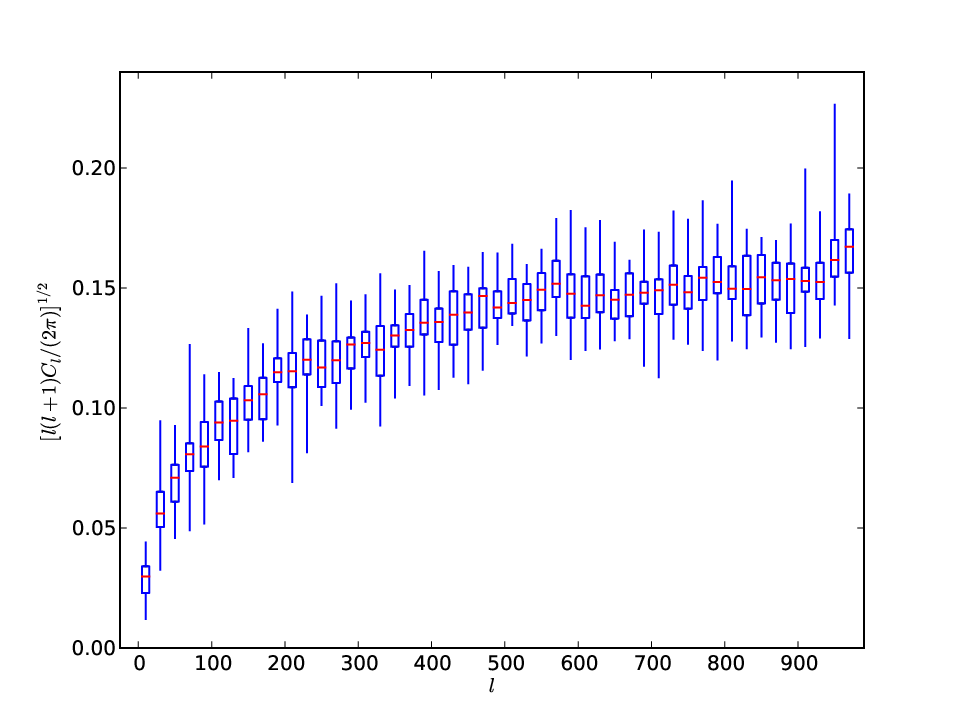
To test the homogeneity and observational character of the data, we calculate the angular power spectrum separately for each stripe, using the method discussed in Section 3. If there is a significant deviation in the angular power spectrum from stripe to stripe, observational systematics might dominate over the real density variations of the combined stripe data that makes our full sample. To test for these systematics, we have calculated angular power spectra of each SDSS stripe from stripe 9 to stripe 37 after masking, with each of the including an identical range of . The angular power spectra from each stripe are remarkably consistent with each other, which is shown in the box-whisker plot in Figure 2, and this shows that these observational systematics do not significantly alter the angular power spectra. The only notable variation between stripes is that the edge stripes 9 and 37 have much larger error bars due to these stripes having the most pixels eliminated due to the seeing and reddening cuts.
We have also varied the seeing and reddening cuts to test their effects. We have varied seeing cuts from 1.0 to 3.0 arcseconds in 0.1 arcsecond intervals, and reddening cuts from 0.1 to 0.5 magnitudes in 0.05 magnitude intervals, but found that neither seeing nor reddening had a significant impact so long as a sufficient galaxy density remained to calculate the angular power spectra. This is consistent with the cross correlations between galaxy density and reddening/seeing calculated by T02 for stripe 10. Nevertheless, to minimize systematics in the SDSS galaxy sample, we have eliminated areas of seeing greater than 1.5 arcseconds and reddening worse than 0.2 magnitudes to be consistent with similar angular correlation function results (Ross et al., 2007), though others have used more stringent cuts (Wang & Brunner, 2012).
2.3 Subsamples
We have chosen our main sample to be from 18th–21st magnitude in the extinction corrected r-band (Stoughton et al., 2002), with the faint limit chosen due to concerns about completeness in the sample past 21st magnitude. Though the 95% completeness r-band magnitude limit is 22.2 (Abazajian et al., 2009), some galaxies at the fainter end of the 21-22 magnitude range are not detected or unusable due to large errors and we choose to limit our analysis to more complete samples.
We have chosen subsamples of our main sample for comparison to previous results, and to test for potential systematic errors on galaxy selection. We first confirm our technique is consistent with the results from T02 up to 21st magnitude, so we have separated stripe 10 into 3 magnitude bins from 18–19, 19–20, and 20–21. The comparison can be expected to be slightly different due to the use of the more complete DR7 data as opposed to the Early Data Release results that used galaxy probabilities (T02), in addition to the photometry calculation difference of magnitudes in SDSS data prior to DR2 (Abazajian et al., 2004). We show these results in Section 4.
We also measure the clustering attributes based on the brightness of the galaxies. The apparently brighter galaxies cluster more strongly and are generally at lower redshift, thus we expect those to have more power in the angular power spectrum. We create three new samples by separating the SDSS galaxies into 3 different r-band magnitude bins from magnitudes 18–19, 19–20, and 20–21. These magnitude ranges are sufficiently bright to minimize the systematic effects of star-galaxy separation and variable sky brightness. These samples have intrinsically different redshift distributions and luminosity functions, therefore the angular power spectra of these samples will reflect these differences, and they are also useful as an important systematic test.
2.4 Simulated Data Set
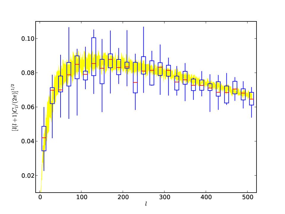
In addition to matching the published results from T02 and verifying that our results from all stripes across the SDSS DR7 are consistent, we performed one additional test of the veracity of our quadratic angular power spectrum estimator. We have generated simulated sky maps and compared the results from our quadratic estimator to the results from the HEALPix11 1 See http://healpix.jpl.nasa.gov angular power spectrum estimator anafast. We first generated a linear angular power spectrum as described in Section 5.1 and used the HEALPix synfast routine to create ten pixelated sky maps at HEALPix resolution 2048. Second, we convert the pixel values in each of these ten sky maps to galaxy overdensities by using the average galaxy density of the SDSS DR7. Third, we mask, in an identical manner to our treatment of the galaxy samples, each of these simulated full sky maps to the stripe 10 boundary as described in Section 3.1.2. Finally, we combine pixels to produce a degraded map with Healpix resolution 256. With these degraded sky maps, we calculate the angular power spectrum by using our quadratic estimator to these ten samples out to .
We also use synfast to generate the same ten maps at Healpix resolution 256, and calculate the angular power spectrum by using HEALPix angular power spectrum estimator anafast to provide a direct comparison to the results from our quadratic estimator. At resolution 256, we use the recommended for synfast and anafast, and performed a standard analysis with anafast of the entire pixelated sky with no regression, masking, or cuts. We show these results along with the results from our quadratic estimator in Figure 3. Both estimators show remarkable agreement, despite the fact that anafast is operating on a full sky map and our quadratic estimator is operating with the Stripe 10 window function. As a result, we feel our implementation of the quadratic estimator and the results we derive are robust.
3 Method
Angular power spectra attempt to measure the multipole moments, , of a two dimensional distribution, in our case the galaxy density (Jaffe et al., 1999). However, since photometric surveys only observe portions of the sky, all multipole moments cannot be individually determined (Tegmark, 1996); what is measured instead is a group of them simultaneously. Multipole moments are grouped into contiguous bands, called bandpowers, and we make the assumption that all moments in the bandpower are equal (e.g., Huterer et al. 2001). The same computation is subsequently performed on the bandpowers as they would normally be on the individual multipole moments. This also serves to reduce the computation needed for the calculation (Borrill, 1999). First, we calculate the angular power spectrum by using the smallest bandpowers possible, and these bandpowers are averaged together into larger bands to improve the signal-to-noise and reduce errors (BJK98).
Typically, Fourier methods are used to describe the distribution of a continuous population, but the galaxy distribution is discrete. To calculate an angular power spectrum, we transform the discrete galaxy counts into a continuous galaxy density distribution. To do this, the sky is divided into “pixels” and the galaxy density in each pixel is calculated. The calculation continues in the same way as it would with a CMB temperature map (e.g., BJK98). Smaller pixels can tell us more information about the angular power spectrum, but the computation required is highly dependent on the number of pixels (Tegmark, 1997).
In this section, we first discuss how we pixelize and mask the data, followed by our selection of bandpowers in Section 3.2. In Section 3.3, we extensively detail how we calculate an angular power spectrum, beginning with KL-compression, the quadratic estimation technique, and the computational difficulty involved in this calculation. In Section 3.4, we describe how these bandpowers can be combined to produce higher signal-to-noise angular power spectrum estimates, and how to calculate the window functions associated with these measurements.
3.1 Pixelization
We have chosen to use a quadratic estimation approach to calculate the maximum likelihood of the angular power spectrum using KL-compression (Bond, 1995; Bunn, 1995). To force the discrete galaxy observations into a continuous population, the sky is pixelated to determine the galaxy overdensity per pixel.
We pixelate the sky using equal area pixels and remove areas that are outside the survey geometry, or have high seeing or reddening values. Any pixels with less than 75% usable area are not considered in the calculation. In the end, the galaxy overdensity is calculated:
| (1) |
where is the galaxy count in pixel , is the average number of galaxies per square degree over the survey area, and is the area of the pixel in square degrees. Thus the data set of possibly millions or more galaxies is reduced to a set of pixels that encodes the galaxy overdensities. The actual choice of pixelization technique, however, is important; and we have tested two different pixelization schemes, each with its own advantages.
3.1.1 Pixelization Schemes
SDSSPix is a hierarchical, equal area pixelization scheme developed specifically for the SDSS by Max Tegmark, Yongzhong Xu, and Ryan Scranton22 2 See http://dls.physics.ucdavis.edu/scranton/SDSSPix/. It uses the natural SDSS stripe geometry to divide the sky into pixels aligned with the SDSS survey coordinates, eta/lambda. Pixels at a particular resolution have a constant width in eta, and a variable width in lambda to satisfy the equal area requirement. While SDSSPix is useful because of the alignment of pixels with survey boundaries which makes seeing and reddening in pixels easier to quantify, the elongation of pixels away from the survey center interfered with the convergence properties of our algorithm described below. This is because elongated pixels smooth density variations preferentially in the direction of elongation while retaining that information in the perpendicular direction. This increases the covariance between the smaller scale modes and drives increasing oscillation in high bandpowers with each iteration.
HEALPix is also a hierarchical, equal area pixelization scheme (Górski et al., 2005), created for CMB experiments such as WMAP and Planck. It divides the sphere into 12 pixels at the base resolution, and higher resolutions recursively quarter these large pixels. The benefit of using HEALPix is that while pixel boundaries have no relation to our observational data, the pixels are not elongated as they are with SDSSPix. Due to the stability of the quadratic estimation method using HEALPix, we have opted to pixelize our data with HEALPix for our calculation.
3.1.2 Pixel Masks
Masking with HEALPix is more complicated than with SDSSPix since pixels may overlap the survey boundaries. For unbiased results, any pixel that overlaps a boundary must not be considered in the calculation since it may have an unphysical overdensity. Thus many pixels on stripe edges are masked. We also eliminate pixels that are not contiguous with the primary SDSS observing footprint. A random sample of 100,000 of the pixels not used due to the boundary are shown in the top panel of Figure 4, we have plotted only a sample to prevent obscuration of the coordinate lines. Furthermore, we must mask pixels due to areas with poor image quality, these pixels are also shown in the bottom of Figure 4. Additionally, we remove pixels where the mean seeing is more than 1.5 arcseconds, and pixels where the mean reddening is greater than 0.2, shown in the top and bottom panels of Figure 5, respectively.


3.2 Selecting Bandpowers
The first step in our approach is to select the initial fine bandpowers. Multipole resolution is limited by , where is the analyzed area’s smallest angular dimension (Peebles, 1980). For this reason, we want the broadest survey possible. Aside from being restricted to choosing bandpowers wider than this limit, the choice of the starting, ending, initial value, and widths of each bandpower is unrestrained, although some choices of initial values may cause non-convergence or singular matrices. We chose initial bandpowers of equal widths, each wide for the full sample and wide for the individual stripes. We use initial values based on a prior angular power spectrum; however, since the quadratic estimation method uses iteration, the final result is fairly insensitive to the input angular power spectrum. We assume all within a band to be constant (Huterer et al., 2001):
| (2) |
where while and zero otherwise, and we define according to standard convention (Bond et al., 2000).
We start with an initial fine binning, to determine where the power is inside the larger bandpowers that we later use. The Fisher information matrix (defined in Equation 8) is used to construct the bandpower window functions, and after we have performed the quadratic estimation to find the maximum likelihood, we will use these window functions to determine the correlation between bandpowers and individual multipole moments .
3.3 Calculating
Using only a knowledge of the survey geometry (or at least the region under consideration) and the assumed values for the bandpowers, we construct the covariance matrix C:
| (3) |
where, S is the signal matrix and N is the noise matrix. The assumed bandpower values will only be approximate, which will make the covariance matrix approximate; but this covariance matrix will be compared to the data and iteratively corrected to converge to the true bandpower values. The signal matrix is calculated directly from the pixelated survey geometry using the assumed set of multipole values . Using Legendre polynomials as the variance window functions, the calculated signal matrix S as shown by Tegmark (1997) is:
| (4) |
where is the angle between pixels and . The exponential factor is introduced to compensate for the smearing caused by a beam of width . For pixels much larger than the beam, as is the case for a galaxy survey, this factor is negligible. The noise matrix, N, is modeled as a Gaussian random process and is diagonal (Huterer et al., 2001):
| (5) |
where is the rms noise in pixel .
3.3.1 Karhunen-Loéve Compression
Rather than perform the full calculation on the vector of overdensities x, we instead choose to transform into a signal to noise basis. This is done by using KL-compression (Vogeley & Szalay, 1996; Tegmark et al., 1997). While this is often useful for data compression, with the high signal in our sample very few modes are discarded due to having greater noise than signal.
We begin by solving the generalized eigenvalue equation:
| (6) |
and normalizing such that . We reorder the vectors by the signal to noise ratio, , in descending order. We discard modes with insufficient signal to noise, and we choose to keep those with . The remaining vectors form the columns of the matrix that we use to transform the data vector , as well as the signal, Legendre polynomial, and noise matrices , , and (T02).
3.3.2 Quadratic Estimation
From the new data vector , we perform the outer product to calculate the observed covariance matrix, , which will be compared to the constructed covariance matrix .
Now that we have a set of bandpowers that we want to determine, we calculate the that have the highest probability of creating the observed data. A complete calculation of the likelihood function, although slow, is possible, but a local maximum can be found by using iteration with the following estimator (BJK98):
| (7) |
where, the Fisher information matrix F is defined as:
| (8) |
Equation 8 provides the mechanism by which we can compare the covariance matrix obtained from the data with the constructed covariance matrix . What this equation accomplishes is retrieving the that produce a covariance matrix that is identical to . Note that we use in Equation 7 as advocated by Tegmark (1998) for uncorrelated error bars and well behaved window functions.
By making an initial estimate of , and iteratively applying this equation, the estimator quickly converges on a maximally probable set of bandpower values. The error in bandpower , given by , is the smallest error any estimator can measure while estimating parameters from the sample itself due to the Cramer-Rao inequality (Kenney et al., 1951; Tegmark, 1997).
3.3.3 Computational Requirements
The quadratic estimation method is computationally complex, due to both a large amount of calculation required for matrix operations as well as large memory requirements to store these matrices. We must consider computational feasability when making choices about the extent of the data that we will analyze. At the scales of interest, we have found the processing time for a single processor scales as:
| (9) |
and the memory requirements scale as:
| (10) |
where , , and are the number of bandpowers, iterations, and pixels respectively. Typically only a few iterations are necessary; we allow 3 iterations to achieve convergence. These are obviously highly dependent on the number of pixels , and processing time and memory requirements become prohibitive much beyond pixels (Borrill, 1999). As a result, we have made use of the National Center for Supercomputing Applications’ (NCSA) 1,024 processor SGI Altix (Cobalt), its successor the 1,536 processor SGI Altix (Ember), as well as the Pittsburg Supercomputing Center’s 768 core SGI Altix (Pople) and 4,096 core SGI UV 1000 (Blacklight) for these calculations.
3.4 Interpreting
3.4.1 Averaging
After defining the bandpowers and calculating the , we use the Fisher Information matrix to determine the correlation between bandpowers (Knox, 1998). Narrow bandpower window functions are preferred so that the error in one band measurement minimally affects other bands.
Though the Fisher matrix and have already been calculated for the choice of bandpowers, we want to have a method of combining bandpowers to improve the signal-to-noise without recalculating using the computationally demanding quadratic estimator method. For this we use the BJK98 method.
First, smaller bandpowers are averaged together into larger bandpowers (not to be confused with the KL-compression matrix B defined earlier) using Equation 11. We can combine any number of adjacent bandpowers to improve signal-to-noise, though combining bandpowers from sections of the angular power spectrum with significant structure will result in a loss of resolution in the areas of interest (BJK98).
| (11) |
| (12) |
The averaged Fisher matrix must be calculated to determine the errors on , which are (Tegmark, 1997).
3.4.2 Calculating Window Functions
To represent the angular power spectrum visually, the data points are characterized not only by the values and errors, but also by the width and position of the bandpowers they represent. The bandpower window functions are given by (T02):
| (13) |
where D is the diagonal matrix that makes the rows of W sum to unity. The midpoints of the bandpowers, , can also be calculated. Algorithmically, is where half the power in the band comes from below and half from above that multipole (BJK98):
| (14) |
| (15) |
We calculate the filter while doing the averaging in Section 3.4.1. This filter function tells us how the power in larger bands is related to the power in the component smaller bands, and gives us information about how the power is distributed within the new larger bands (BJK98). The edges of the band, and , are defined to be where drops to of the peak power, and we plot these as horizontal error bars. The angular power spectrum at can be plotted with horizontal error bars ranging from to , with value and vertical error bars .
4 The SDSS Angular Power Spectrum
The results of our angular power spectrum calculation for stripe 10 for are shown in the top panel of Figure 6, separated by magnitude. Though our results are consistently higher than those in T02 in all samples, we find that our results are still in agreement. This is due to a known magnitude calculation error in early SDSS data, which miscalculated galaxy model magnitudes by roughly 0.2 mag (Abazajian et al., 2004). When we shift the samples by 0.2 magnitudes to account for this difference, our results match very well with the previous results, typically within one standard deviation as shown in the bottom panel of Figure 6. Additionally, as we are using DR7 instead of the EDR, galaxy counts versus galaxy probabilities, and HEALPix rather than SDSSPix, we do not expect the results to exactly coincide.
In addition, we not only need to know the final , but to completely characterize the errors and the structure of each bandpower, we need to know the window functions. The variance and covariance of the are derived from the Fisher matrix, and the bandpower window functions show what the power in a band comes from, so we prefer bandpower window functions to be as narrow as possible. For illustration and comparison to T02, the bandpower window functions for the 18–19 magnitude bin of stripe 10 are shown in the top panel of Figure 7. We see that at about , the window functions become wider signifying that our signal has dropped below shot noise fluctuations, so bands beyond that are not used. In the other magnitude bins, our signal does not drop below shot noise fluctuations out to such as in the bottom panel of Figure 7. The window functions for other stripes are similar, and we have made these available online33 3 All results discussed in this paper are available at :.
The results of the angular power spectrum of our entire sample for , as well as for our magnitude separated subsamples, are summarized in Figure 8 and in Table 1. The brightest and on average closest galaxies in the 18–19 r-band magnitude bin are the most highly clustered at all as expected. Below that is the 19–20 magnitude bin, and the least clustered at all is the 20–21 magnitude bin. Also plotted are the linear theoretical angular power spectra discussed in Section 5.1 for .


| Sample | 18–21 | 18–19 | 19–20 | 20–21 | |||
|---|---|---|---|---|---|---|---|
| 3 | 0.00030 0.00020 | 3 | 0.00035 0.00029 | 3 | 0.00035 0.00025 | 3 | 0.00032 0.00020 |
| 9 | 0.00072 0.00020 | 9 | 0.00240 0.00062 | 9 | 0.00110 0.00030 | 9 | 0.00053 0.00015 |
| 19 | 0.00129 0.00028 | 19 | 0.00393 0.00082 | 19 | 0.00199 0.00043 | 19 | 0.00114 0.00024 |
| 30 | 0.00393 0.00061 | 29 | 0.00977 0.00158 | 30 | 0.00605 0.00094 | 30 | 0.00301 0.00047 |
| 40 | 0.00409 0.00058 | 40 | 0.01167 0.00169 | 40 | 0.00593 0.00087 | 40 | 0.00343 0.00048 |
| 49 | 0.00475 0.00062 | 50 | 0.01254 0.00168 | 49 | 0.00800 0.00104 | 49 | 0.00366 0.00049 |
| 60 | 0.00581 0.00069 | 59 | 0.01430 0.00178 | 60 | 0.00860 0.00105 | 60 | 0.00484 0.00058 |
| 72 | 0.00571 0.00051 | 72 | 0.01339 0.00129 | 72 | 0.00861 0.00078 | 73 | 0.00479 0.00043 |
| 87 | 0.00601 0.00050 | 88 | 0.01519 0.00136 | 87 | 0.00858 0.00074 | 87 | 0.00494 0.00042 |
| 103 | 0.00698 0.00054 | 103 | 0.01638 0.00139 | 102 | 0.01053 0.00084 | 103 | 0.00546 0.00043 |
| 117 | 0.00795 0.00057 | 117 | 0.01653 0.00139 | 117 | 0.01098 0.00084 | 117 | 0.00675 0.00049 |
| 132 | 0.00853 0.00059 | 133 | 0.01987 0.00156 | 132 | 0.01201 0.00088 | 132 | 0.00673 0.00048 |
| 147 | 0.00891 0.00059 | 147 | 0.02014 0.00159 | 147 | 0.01126 0.00083 | 148 | 0.00746 0.00051 |
| 163 | 0.00871 0.00056 | 162 | 0.02076 0.00166 | 163 | 0.01256 0.00088 | 163 | 0.00662 0.00045 |
| 177 | 0.00997 0.00061 | 177 | 0.02135 0.00175 | 177 | 0.01314 0.00090 | 177 | 0.00789 0.00050 |
| 190 | 0.01018 0.00078 | 190 | 0.02387 0.00262 | 190 | 0.01231 0.00111 | 190 | 0.00843 0.00070 |

5 Theory
5.1 Theoretical Power Spectra
The statistical characterizations of galaxy clustering provided by our angular power spectrum measurements are only the first step. In order to constrain models of structure formation, we must compare these results to theoretical linear angular power spectra. To obtain theoretical , we project the linear 3D power spectrum , modeled with the fitting formulae of Eisenstein & Hu (1998), down to two dimensions. With , we can calculate the we expect from a given theory (e.g., Huterer et al. 2001). From Crocce et al. (2010) we have the exact calculation for the theoretical linear angular power spectrum:
| (16) |
where:
| (17) |
| (18) |
where is the growth function (Carroll et al., 1992) and are Bessel functions, is the bias, and and are the comoving distance and number density respectively. This simplifies if we use Limber’s approximation (Limber, 1953) to simplify the calculation of the Bessel functions:
| (19) |
The theoretical power spectrum depends only on cosmological parameters through the 3D power spectrum and the bias, so we can use this dependence to infer constraints on these values. The only knowledge it requires about the sample is the redshift distribution. We calculate the redshift distribution by assuming the redshift of each galaxy is distributed as a Gaussian with mean equal to the observed photometric redshift and standard deviation equal to the error of the photometric redshift. We sample the distribution of each galaxy and then weight by volume and luminosity function constraints as in Ross et al. (2010) with the luminosity function of Montero-Dorta & Prada (2009).
In Figure 9, we show the photometric redshift distribution of our main sample of over 18 million galaxies, separated into photometric redshift bins of width 0.001 with . We see that the peak of the sample is at and falls off rapidly past . The redshift distribution is important because we must use it when we project the 3D power spectra to compare to our angular power spectra. Also in Figure 9, we have separated the redshift distribution into magnitude bins, and see the variations of photometric redshift distributions by magnitude, with the brighter bins being on average closer than the fainter bins. The average redshifts of these samples are for the 18–19 magnitude bin, for 19–20, for 20–21, and for the entire sample.
5.2 Fitting Theory to Data
To constrain cosmological parameters, we use a fitting technique to determine the calculated theoretical linear angular power spectrum that best fits the observed bandpower measurements (Tegmark, 1997). First, an average over the chosen bandpowers of the newly calculated is made so that these can be compared (Knox, 1999):
| (20) |
with the bandpower window function from Equation 13. We evaluate the following where F is the Fisher matrix and are the cosmological parameters (Bond et al., 2000):
| (21) |
We assume a flat cosmology and the WMAP baryon to matter ratio of (Larson et al., 2011) to perform this minimization for . Over this range, the equivalent k is less than 0.16 h/Mpc at our median redshift of ; and, we therefore expect the linear to be a good approximation. We note that, given the limited range of the data used with this cut, the restriction is not likely to yield competitive constraints on , and to fit the data past we would need to use a non-linear power spectrum. Indeed, we find a wide range of allowed values, which we illustrate by displaying the results of our minimization for the 18–21 magnitude sample in Figure 10. We find our best fit and for the 18–21 sample, and for the 18–19 magnitude subsample, and for the 19–20 magnitude subsample, and and 20–21 magnitude subsample. We display these best-fit models against our measurements in Figure 8.

6 Discussion
Comparing the observed angular power spectrum to a linear theoretical spectrum is not expected to provide strong constraints on since varying primarily changes the angular power spectrum at higher . Though weakly constrained, these measurements of are consistent with other recent measurements of from galaxy angular power spectra such as Huterer et al. (2001); Frith et al. (2005); Blake et al. (2007); Thomas et al. (2010), as well as measurements through other methods such as the 7-year WMAP results from the cosmic microwave background (Larson et al., 2011). This agreement confirms that the samples of galaxies and the measurement techniques we use have no large systematic errors.
If we assume that the primordial fluctuations that seeded the large scale structure that we see today were Gaussian (e.g., Guth 1981), the angular power spectrum contains all clustering information on linear scales. However, there has been some evidence that this might not be the case (e.g., Elsner & Wandelt 2010). Furthermore, non-linear effects from gravitational collapse become more pronounced at higher , which also causes a departure from Gaussianity. Though the quadratic estimator we employ assumes Gaussian fluctuations, the maximum likelihood angular power spectrum values we determine are unaffected by potential non-Gaussianities in the galaxy density field. We note, however, that the presence of such non-Gausianities would generally cause us to underestimate our error bars (T02).
As we estimate the mean galaxy density from the survey itself, we constrain the data vector x to have zero mean; this is known as the integral constraint (see Tegmark et al. 1998 for a detailed discussion). If we fail to account for the integral constraint we can underestimate the power on large scales (Huterer et al., 2001), so we correct for this by adding a large number to the mean mode in the noise matrix N before KL-compression. The KL-compression stage will determine that the signal-to-noise of the mean mode is low and it will be discarded with other low signal-to-noise modes.
The major limitation of our adopted approach for the calculation of the galaxy angular power spectrum is the computational difficulty. The signal-to-noise of the SDSS DR7 is sufficient to calculate the angular power spectrum to smaller scales than we have here, but doubling the resolution quadruples the number of pixels to . Since the matrix muliplication and inversion scales as , doubling the resolution is a 64-fold increase in computation, which is beyond our current computational resources, though we are looking into the possibility of performing this calculation, perhaps by KL-compressing the data even further.
We have also explored using alternative platforms to accelerate the computation. We have implemented this method on Graphics Processing Units (GPUs), which are part of every modern personal computer. GPUs are specifically designed to parallelize simple computations across many small multiprocessors, which make it ideal for vector and matrix calculations. Using an Nvidia 8800 GTX and transferring the matrix operations to the GPU, while the rest of the code ran on the CPU, proved to be very effective at accelerating the quadratic estimation section of this calculation, speeding it up by a factor of 337. For this to be effective, however, the matrices had to fit into the relatively small on board memory of the GPU, which in our test system was 768 MB. In comparison, the memory required by the calculation performed in this paper was roughly 75 GB. So while this platform seems very promising in accelerating this computation, the memory available will not be sufficient in the near future to allow us to meet or exceed the calculations that can be performed using current supercomputers.
While important, this work has merely been the first step. By applying this method to volume-limited samples, we can constrain the redshift evolution of the galaxy angular power spectrum. In addition, we can use the photometric galaxy type classification to distinguish differences in the clustering properties of early- and late-type galaxies in different redshift shells. Furthermore, by utilizing a full 3D, nonlinear theoretical power spectrum, we can model our measurements to higher values and make more stringent measurements of cosmological parameters and we plan on taking these steps in a future work.
7 Conclusions
We have used the quadratic estimation method with KL-compression to determine the SDSS DR7 angular power spectrum, first as a means of radical compression of the angular clustering information, and second to match these observed angular power spectra with theoretical angular power spectra to extract the linear bias and cosmological matter density. We masked for observational effects and applied this method to over 18 million SDSS DR7 galaxies and three magnitude subsamples out to . We also measured the angular power spectrum for each individual stripe out to for stripes 9–37. We have used the photometric redshift distribution of these galaxies to project the 3D power spectrum to two dimensions to obtain theoretical linear angular power spectrum, and used minimization to determine the best fit parameters given the observations. As the linear angular power spectrum approximation is not valid for the entire range of our estimated angular power spectrum, these parameter constraints have a large allowed range of values.
We found that the linear bias of our samples was in the 18–19 magnitude range, for 19–20, and for 20–21, with an overall bias of for our combined 18–21 magnitude sample. We have also calculated the cosmological density of matter as from our entire sample.
Acknowledgements
The authors would like to thank Adam Myers, Dragan Huterer, Lloyd Knox for their valuable discussion and advice, and the referee for suggestions that have greatly improved the manuscript.
This research was supported in part by the National Science Foundation through XSEDE resources provided by Pittsburgh Supercomputing Center’s 4,096 core SGI UV 1000 (Blacklight) and 768 core SGI Altix (Pople) as well as the 1,024 processor SGI Altix (Cobalt) and 1,536 processor SGI Altix (Ember) of the National Center for Supercomputing Applications.
Funding for the SDSS and SDSS-II has been provided by the Alfred P. Sloan Foundation, the Participating Institutions, the National Science Foundation, the U.S. Department of Energy, the National Aeronautics and Space Administration, the Japanese Monbukagakusho, the Max Planck Society, and the Higher Education Funding Council for England. The SDSS Web Site is http://www.sdss.org/.
The SDSS is managed by the Astrophysical Research Consortium for the Participating Institutions. The Participating Institutions are the American Museum of Natural History, Astrophysical Institute Potsdam, University of Basel, University of Cambridge, Case Western Reserve University, University of Chicago, Drexel University, Fermilab, the Institute for Advanced Study, the Japan Participation Group, Johns Hopkins University, the Joint Institute for Nuclear Astrophysics, the Kavli Institute for Particle Astrophysics and Cosmology, the Korean Scientist Group, the Chinese Academy of Sciences (LAMOST), Los Alamos National Laboratory, the Max-Planck-Institute for Astronomy (MPIA), the Max-Planck-Institute for Astrophysics (MPA), New Mexico State University, Ohio State University, University of Pittsburgh, University of Portsmouth, Princeton University, the United States Naval Observatory, and the University of Washington.
Some of the results in this paper have been derived using the HEALPix (Górski et al., 2005) package.
References
- Abazajian et al. (2009) Abazajian, K. N., et al. 2009, ApJS, 182, 543
- Abazajian et al. (2004) Abazajian, K., et al. 2004, AJ, 128, 502
- Blake et al. (2004) Blake, C., Ferreira, P. G., & Borrill, J. 2004, MNRAS, 351, 923
- Blake et al. (2007) Blake, C., Collister, A., Bridle, S., & Lahav, O. 2007, MNRAS, 374, 1527
- Brunner et al. (2000) Brunner, R. J., Szalay, A. S., & Connolly, A. J. 2000, ApJ, 541, 527
- Bond (1995) Bond, J. R. 1995, Physical Review Letters, 74, 4369
- Bond et al. (1998) Bond, J. R., Jaffe, A. H., & Knox, L. 1998, Phys. Rev. D, 57, 2117
- Bond et al. (2000) Bond, J. R., Jaffe, A. H., & Knox, L. 2000, ApJ, 533, 19
- Borrill (1999) Borrill, J. 1999, 3K cosmology, 476, 277
- Bunn (1995) Bunn, E. F. 1995, Ph.D. Thesis,
- Carroll et al. (1992) Carroll, S. M., Press, W. H., & Turner, E. L. 1992, ARA&A, 30, 499
- Crocce et al. (2010) Crocce, M., Cabre, A., & Gaztañaga, E. 2010, arXiv:1004.4640
- Csabai et al. (2007) Csabai, I., Dobos, L., Trencséni, M., Herczegh, G., Józsa, P., Purger, N., Budavári, T., & Szalay, A. S. 2007, Astronomische Nachrichten, 328, 852
- Eisenstein & Hu (1998) Eisenstein, D. J., & Hu, W. 1998, ApJ, 496, 605
- Elsner & Wandelt (2010) Elsner, F., & Wandelt, B. D. 2010, ApJ, 724, 1262
- Frith et al. (2005) Frith, W. J., Outram, P. J., & Shanks, T. 2005, MNRAS, 364, 593
- Górski et al. (2005) Górski, K. M., Hivon, E., Banday, A. J., Wandelt, B. D., Hansen, F. K., Reinecke, M., & Bartelmann, M. 2005, ApJ, 622, 759
- Gunn et al. (1998) Gunn, J. E., et al. 1998, AJ, 116, 3040
- Guth (1981) Guth, A. H. 1981, Phys. Rev. D, 23, 347
- Huterer et al. (2001) Huterer, D., Knox, L., & Nichol, R. C. 2001, ApJ, 555, 547
- Jaffe et al. (1999) Jaffe, A. H., Bond, J. R., Ferreira, P. G., & Knox, L. E. 1999, 3K cosmology, 476, 249
- Kenney et al. (1951) Kenney, J., & Keeping, E. 1951, Mathematics of Statistics, Part 2
- Knox (1998) Knox, L. 1998, Eighteenth Texas Symposium on Relativistic Astrophysics, 282
- Knox (1999) Knox, L. 1999, Phys. Rev. D, 60, 103516
- Larson et al. (2011) Larson, D., et al. 2011, ApJS, 192, 16
- Limber (1953) Limber, D. N. 1953, ApJ, 117, 134
- Lupton et al. (2001) Lupton, R., Gunn, J. E., Ivezić, Z., et al. 2001, Astronomical Data Analysis Software and Systems X, 238, 269
- Maddox et al. (1990) Maddox, S. J., Efstathiou, G., Sutherland, W. J., & Loveday, J. 1990, MNRAS, 243, 692
- Montero-Dorta & Prada (2009) Montero-Dorta, A. D., & Prada, F. 2009, MNRAS, 399, 1106
- Myers et al. (2007) Myers, A. D., Brunner, R. J., Nichol, R. C., Richards, G. T., Schneider, D. P., & Bahcall, N. A. 2007, ApJ, 658, 85
- Netterfield et al. (2002) Netterfield, C. B., et al. 2002, ApJ, 571, 604
- Oh et al. (1999) Oh, S. P., Spergel, D. N., & Hinshaw, G. 1999, ApJ, 510, 551
- Peebles (1973) Peebles, P. J. E. 1973, ApJ, 185, 413
- Peebles (1980) Peebles, P. J. E. 1980, Research supported by the National Science Foundation. Princeton, N.J., Princeton University Press, 1980. 435 p.,
- Ross et al. (2007) Ross, A. J., Brunner, R. J., & Myers, A. D. 2007, ApJ, 665, 67
- Ross et al. (2010) Ross, A. J., Percival, W. J., & Brunner, R. J. 2010, MNRAS, 407, 420
- Ross et al. (2011) Ross, A. J., Ho, S., Cuesta, A. J., et al. 2011, MNRAS, 417, 1350
- Skrutskie et al. (2006) Skrutskie, M. F., et al. 2006, AJ, 131, 1163
- Smoot et al. (1992) Smoot, G. F., et al. 1992, Astrophys. J, Lett., 396, L1
- Spergel et al. (2007) Spergel, D. N., et al. 2007, ApJS, 170, 377
- Stoughton et al. (2002) Stoughton, C., et al. 2002, AJ, 123, 485
- Tegmark (1996) Tegmark, M. 1996, MNRAS, 280, 299
- Tegmark (1997) Tegmark, M. 1997, Phys. Rev. D, 55, 5895
- Tegmark et al. (1997) Tegmark, M., Taylor, A. N., & Heavens, A. F. 1997, ApJ, 480, 22
- Tegmark (1997) Tegmark, M. 1997, Phys. Rev. D, 56, 4514
- Tegmark (1998) Tegmark, M. 1998, Eighteenth Texas Symposium on Relativistic Astrophysics, 270
- Tegmark et al. (1998) Tegmark, M., Hamilton, A. J. S., Strauss, M. A., Vogeley, M. S., & Szalay, A. S. 1998, ApJ, 499, 555
- Tegmark et al. (2002) Tegmark, M., et al. 2002, ApJ, 571, 191
- Thomas et al. (2010) Thomas, S. A., Abdalla, F. B., & Lahav, O. 2010, arXiv:1011.2448
- Vogeley & Szalay (1996) Vogeley, M. S., & Szalay, A. S. 1996, ApJ, 465, 34
- Wang & Brunner (2012) Wang, Y., & Brunner, R. J. 2012, in preparation.