Complex network classification using partially self-avoiding deterministic walks
Abstract
Complex networks have attracted increasing interest from various fields of science. It has been demonstrated that each complex network model presents specific topological structures which characterize its connectivity and dynamics. Complex network classification rely on the use of representative measurements that model topological structures. Although there are a large number of measurements, most of them are correlated. To overcome this limitation, this paper presents a new measurement for complex network classification based on partially self-avoiding walks. We validate the measurement on a data set composed by 40.000 complex networks of four well-known models. Our results indicate that the proposed measurement improves correct classification of networks compared to the traditional ones.
Keywords:
complex networks, deterministic walks, networks classification, networks measuresI Introduction
Due to the development of informatics, the acquisition of huge data sets has become possible. The analysis of these huge data sets migrated from few individual components (nodes) to a huge number of components all of them interconnected (links) [1]. It has been noticed that many systems have physically close nodes highly connected and distant nodes are weakly connected. As a consequence, a new type of topological structure emerged [2, 3, 4]. This new structure interpolates the regular lattice and the random (Erdõs and Rényi) one [5, 6]. This change of paradigm has made the junction of the mathematical graph formalism (associated to finite systems) with the statistical physics analysis in a new type of topological structure, which has been named complex network. It has been realized that the complex networks can describe several types of topological structures of our daily lives ranging from informatics systems (computer connections in www or internet pages referencing) to biology (protein structures [7], metabolic networks) passing through social systems (scientific citation [8], actors network, disease and rumor propagation, linguistics [9] etc.), and pattern recognition [10, 11, 12, 13].
To use complex networks formalism in a given system, one must firstly specify which parts of the system form the nodes and how these nodes are interconnected. It has been shown that completely different real systems may share a common topological structure. Thus, one is concerned in how to differentiate them through topological measurements [11].
For a robust network classification, representative measures must be extracted. The problem is how to define a set of measures that is the most appropriate for a specific application. Several measures have been proposed such as the average number of connections of a node [10, 14], hierarchical degree [15, 14], clustering coefficient [14], assortativity etc. Nevertheless, many of these measures are correlated, leading to redundancy [14]. Although optimal results are not guaranteed, the use of statistical methods (such as principal component analysis or linear discriminant analysis) to select and improve the measure set is an alternative to solve redundancy and subjective selection [14].
Here we propose to consider networks, with each link having a weight (weighted network) and to use of a new way to classify them. We propose to use agents that leave from each node and go to the closest neighbor (the smallest link weight) that has not been visited in the preceding time steps. This partially self-avoiding deterministic rule can be modified so that the agent goes to the furthest (the strongest link weight, instead of the closest one) neighbor at each time step. Although the partially self-avoiding walk rules are simple, the agent trajectories are complicated and lead to an effective exploration of the network. The closest (furthest) neighbor rule produces trajectories that explore locally (globally) the network. In this study, the partially self-avoiding walks have been applied to classify four kinds of networks: Erdõs-Rényi, geographical, small-world and scale-free. This simple procedure allows our method to achieve results in network classification that are better than the traditional ones. We call attention that a similar technique has been successfully employed in the classification of image texture [16].
This paper is organized as follows. In Sec. II, a brief review of the results of partially self-avoiding walks is presented. In Sec. III, we describe the partially self-avoiding walk methods for network classification. Numerical experiments and results are presented in Sec. V. Finally, in Sec. VI, concluding remarks and possible extensions of the method are presented.
II Partially Self-avoiding Walk
Random walks in regular or random environment have been extensively studied [17, 18]. Nevertheless, deterministic walks in regular [19, 20] or random [21] environments also present interesting results. These results can be applied to a whole variety of practical situations such as: image analysis [22, 16, 23], pattern recognition [24], fractal [25], thesaurus dictionaries [26], optimization [27], etc.
For instance, consider a partially self-avoiding deterministic walk, where an agent wishes to visit points randomly distributed in a map of dimension. These points can be considered as sites and the agent can move from one to another following the rule of, at each discrete time step, going to the nearest site not visited in the previous steps. The agent performs a partially self-avoiding walk, where the self-avoidance is limited to the memory window . Although the dynamical deterministic rule is simple, the agent trajectory can be very complicated [28, 29].
The agent movements depends strictly on the data set configuration and on the starting site [28, 29]. They are entirely performed based on a neighborhood table, so that the distances among the sites are simply a way of ranking their neighbors. This feature leads to an invariance in scale transformations [24]. Starting from given point, the trajectory starts with the agent visiting preferentially new points and ends in a cycle, where the same sequence of points are visited (see Fig. 1). The beginning of the trajectory has a transient time and the ending cycle has a period of or a -attractor. Notice that and/or are different for different starting points so that a transient time and attractor period joint distribution can be computed for the generated trajectories. One obtains the same trajectories for the same point configuration regardless the scale one is dealing.
The most trivial case to deal with the deterministic agent is to consider . The agent remains in the same site and the trajectory has null transient time and an attractor with period . The transient time cycle period joint distribution is simply given by: , where is the Kronecker delta. Despite its triviality, this becomes interesting because it is the simplest situation of a stochastic version of this partially self-avoiding walk [30, 31, 32].
For a memoryless agent (), at each time step, the agent must leave the current site and go to the nearest one. After a very short transient time, the agent becomes trapped by a couple of mutually nearest neighbors. The transient time and period joint probability distribution, for , can be analytically calculated [33]: , where is the gamma function and is the normalized incomplete beta function. In the limit , one is able to calculate it analytically [34]:
| (1) |
When greater values of are considered, the cycle distribution is no longer peaked at , but presents a whole spectrum of cycles with period [28, 29, 35, 34, 36].
Another possible way to deal with these partially self-avoiding deterministic walks is to consider a two dimensional lattice and randomly distribute random weights to the nearest neighbors so that a given agent, with memory , explore the lattice. This system is depicted in Fig. 1.

III Complex Network Modeling
Below we describe how this partially self-avoiding walks can be used to classify networks. We start presenting how to perform these walks on networks. Next we use the transient time cycle period joint distribution to create a vector that characterizes the topology of the network.
III.1 Partially Self-avoiding Walks on Networks
Consider a network represented by a set of vertices and a set of links , where each component represents the link weight that connects vertex to vertex . Yet, is a set such that all elements are neighbor of the vertex and is a vertex list that store the agent trajectory.
The agent starts the trajectory in a vertex . Following the rule of going to the nearest vertex that has not been visited in the previous steps, the agent build his trajectory. On networks, the movements taken by the agent are completely performed with respect to the set of link weights and the memory (Eq.2). The memory is a subset composed of the last visited vertices of the trajectory
| (2) |
Since weight equalities may occur and the agent does not know where to go, one creates the set:
| (3) |
to represent a set of vertices, so that these vertices are the closest (with respect to the weights) to the given vertex and do not belong to the memory set . Depending on the chosen movement rule, at each time step, the agent leaves its vertex and go to the nearest one (defined by ) or furthest one (switching por in Eq. 3). The trajectory is iterated by Eqs. 3 and 4.
To solve possible equalities in , if has only one element, this is chosen as the following vertex to the agent. Otherwise, the equality is solved by a function that returns only a vertex. This function may return a vertex randomly chosen or execute a more sophisticated operation
| (4) |
After a transient time , the agent is trapped in an attractor with period . The trajectory can be iterated up to a determined number of steps and it searches for an attractor, or at each time step, determine if an attractor has been reached and finish the trajectory. The attractor detection is defined by
| (5) |
considering as the vertex index , i.e. . If , an attractor with period and transient time have been detected. If , the agent has not found any attractor and with . An efficient computational strategy to find attractors can be found in Ref. [16].
III.2 Signature Vector
The transient time and cycle period joint distribution stores a great quantity of information concerning the partially self-avoiding deterministic walk in a given environment. To effectively use these walks, relevant information must be extracted from . This relevant information is stored in a signature vector , where represents the dynamics adopted, for instance, the agent going to the nearest or furthest vertex.
An important issue raised about the partially self-avoiding deterministic walk concerns the movement rule adopted by the considered agent. On one hand, agents guided for the shorter distance are appropriate to find attractors in regions with high homogeneity. On the other hand, agents guided for the highest distance find attractors located in regions with low homogeneity. The use of different movement rules reflect in different joint distributions, allowing the use of information from various sources in the environment characterization [16]. Trajectories produced by different rules on a graph have distinct patterns for the same graph, as can be seen in Fig. 2. In this work, only two movement rules were used: , the agent moves to the furthest vertex and , the agent moves to the nearest vertex.


The signature vector is supposed to characterize the environment where the walks have been performed. To compose the signature vector, an interesting strategy is to built a histogram [16] from the joint distribution. This histogram represents the number of walks that has a length of , where and are the transient time and period of the attractor, respectively. From the histogram, descriptors are used to compose the signature vector ,
| (6) |
The first descriptor is on position , because there is no smaller period.
The joint distribution depends on the value of and the movement rule . To capture information from different sources and scales, a signature vector consisting of the concatenation of with multiples values and different movement rules is built:
| (7) |
The algorithm for the proposed measurement is presented below. First, walks are performed on a complex network with different memories () and movement rules . Thus, a joint distribution is obtained. For each joint distribution, a histogram is calculated and a feature vector is built. Finally, the vector of each value of memory and movement rule are concatenated, obtaining a final feature vector with information from various sources and scales.
IV Analysis of the Proposed Method
In this section, we present an analysis of the proposed method with regard to the complex network features, such as average degree and number of vertices. In Fig. 3, histograms of walk length for complex network models built using and vertex degree mean are presented. For purpose of comparison, each column represents an iteration of the same model and each row represents a complex network model. It is possible to note that the histograms present distinct patterns and therefore, we can conclude that the walks can be used to characterize each complex network model. Table 1 shows four statistics calculated from the histograms. From this table, it is shown that the mean of the walk lengths on the scale-free model is the longest. It occurs because most vertices have few connection, which makes difficult to identify attractors. On the other hand, the mean of the walk lengths on the geographical networks is the shortest. In geographical networks, the vertices are connected in proportion to spatial distance, which helps to formation of groups of connected vertices and thus the identification of attractors.


| Statistics of Histograms | ||||
|---|---|---|---|---|
| Model | Mean | Standard Deviation | Entropy | Skewness |
| Small-world | 27.83 | 24.12 | -5.97 | 1.72 |
| Erdõs-Rényi | 85.57 | 57.42 | -7.66 | 0.64 |
| Geographical Network | 17.88 | 10.50 | -5.19 | 1.08 |
| Scale-free | 106.02 | 40.59 | -7.16 | -0.18 |
Figure 4 illustrates the effect on the histograms for ranging from to while keeping on the small-world model. The histograms are similar as we increase the number of vertices. For the small-world network, the histograms show a peak on walks of small length and decay as the walk length is increased. As an example, the mean, standard deviation, entropy, skewness and kurtosis of the histograms are given in Table 2.


| Statistics of Histograms | ||||
|---|---|---|---|---|
| Mean | Standard Deviation | Entropy | Skewness | |
| 27.89 | 23.76 | -5.97 | 1.59 | |
| 25.05 | 19.02 | -5.80 | 1.39 | |
| 26.98 | 22.09 | -5.93 | 1.66 | |
| 26.52 | 21.96 | -5.89 | 1.71 | |
| 26.28 | 20.95 | -5.88 | 1.64 | |
The histograms of walk lengths for different values of are shown in Figure 5. As we increase the values of , the peak of walks with short length is smoothened. For high values of , the vertices become more connected and it undermines the traveller in search of an attractor. Then, walks with longer lengths can be generated more frequently. Table 3 presents the histogram statistics for different values of .


| Statistics of Histograms | ||||
| Mean | Standard Deviation | Entropy | Skewness | |
| 30.86 | 23.11 | -6.14 | 1.35 | |
| 41.53 | 31.96 | -6.61 | 1.83 | |
| 48.61 | 33.84 | -5.83 | 0.91 | |
| 58.01 | 39.68 | -7.07 | 0.76 | |
V Experiments and Results
To evaluate partially self-avoiding deterministic walks as a complex network measurement, experiments were performed on a data set composed by 40.000 artificial networks. The complex network models considered in this data set include: Erdõs-Rényi, small-world, geographical network and scale-free. The data set consists of artificial complex networks built with random weight for the edges, number of vertices ranging from to increasing by steps of , and average degree ranging from to increasing by steps of . For the geographical network, the vertices were random and uniformly distributed inside a square box.
As in Ref. [16], descriptors from the histogram have been used to compose the signature vector. The statistical analysis reveals that relevant information is concentrated only in the first few elements. The signature vector from each complex network were classified using KNN classifier [37] () in a 10-fold cross-validation strategy. Since our focus is on modeling, we use a simple classifier rather than a more sophisticated classifier such as support vector machines which have been shown to produce superior results but requires more tuning of parameters.
V.1 Parameters Evaluation
An evaluation of parameters of the partially self-avoiding deterministic walks is presented in the following. Classification results for different values of and movement rule are presented in Table 4. In most cases, movement rule achieved better classification results than rule . The former found attractors in homogeneous and local regions, i. e. regions where the edge weights are low. Figure 6 shows the Principal Component Analysis (PCA) projection considering two dimensions for both movement rules. As we can see, the potential of the movement rule to obtain separated clusters is evident from this example. Another important result is that the concatenation of both rules () increased the correct classification rate. This is because the strategy keeps local and global information from the complex network, providing a powerful framework to complex network characterization.
| Memory () | ||||||
|---|---|---|---|---|---|---|
| 0 | 1 | 2 | 3 | 4 | 5 | |
| 74.31 | 87.27 | 73.86 | 64.45 | 61.59 | 58.45 | |
| 76.2 | 81.26 | 70.98 | 63.21 | 58.94 | 55.76 | |
| 84.07 | 93.02 | 84.03 | 74.84 | 68.37 | 61.09 | |


Results from Table 4 also showed that for both movement rules, the correct classification rate is decreased as the memory is increased, except for which is the trivial case of the deterministic walk. These results lie on the fact that a walk has more difficulty, as the memory increases, in finding an attractor in the image [16]. On the other hand, small values of memory perform a better local analysis of the network structure, resulting in an higher correct classification rate. As an illustration, Figure 7 presents the first two PCA discriminant for different values of memory.


Results using signature vectors composed by the concatenation of multiple values of memory are presented in Table 5. This strategy diminishes the importance of individual values of and allows walks with a higher range of lengths, thus providing more robust characterization. In Figure 8, PCA projection of signature vectors composed by multiple values of () is shown.
| Memories () | |||
|---|---|---|---|
| 95.49 | 94.23 | 98.11 | |
| 95.65 | 94.47 | 98.16 | |
| 95.73 | 94.68 | 98.19 | |
| 95.66 | 94.82 | 98.21 | |
| 95.65 | 94.83 | 98.22 |

V.2 Multivariate Analysis of Variance
Here, we determine whether the means of the feature vectors differ significantly among the four classes of complex networks. To answer this question, we apply the multivariate analysis of variance (MANOVA) [38]. The MANOVA takes a set of grouped data composed by the features extracted using the partially self-avoiding walks characteristics. First, we generate 1000 complex networks for each class (random network, scale-free, geographical and small-world). For each complex network, from the histogram of the partially self-avoiding walks and extract the feature vector as in the previous experiments. Thus, one has a data matrix of 4000 rows (1000 samples for each class) and 60 columns (features). Figure 9 depicts the scatter plot matrix for the first four features. On the bottom panel, the figure shows the box plots for different classes.

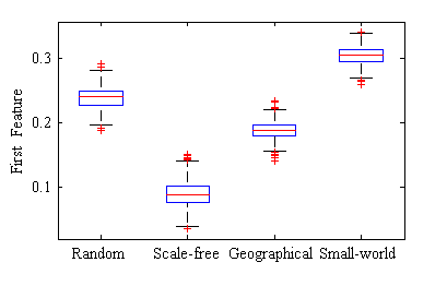
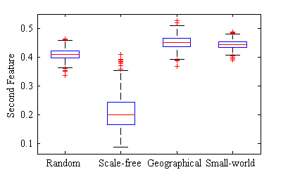
Considering the means of the four classes by , we perform the MANOVA to test the hypothesis that . The test of homogeneity (equality) of variance is performed. Once the variances are equal, the means are tested and the hypothesis of equal means is rejected even at the 1% significance level.
In Figure 10, we generate a dendrogram of the class means after the MANOVA. To obtain the dendrogram, the single linkage method is applied in the matrix of Mahalanobis distances between class means. The ordenate represents the distance in which two classes is connected. In this way, one observes that the random network and the geographical network produce features with the most similar characteristics. Also, the scale-free is the network which produce the most different features from the other three networks. These results is corroborated by the plots of Figure 9.

V.3 Correlation with Traditional Measures
The network classification obtained with the partially self-avoiding deterministic walks are compared to the traditional methods. The results of these comparisons are shown in Table 6. For each traditional measurement for each vertex, the mean value and its standard deviation are estimated. Results of in Table 6 indicate that the classification rate improves with our proposed method from 78.32% to 98.24% over the coefficient clustering measurement. The next highest rate of 71.87% is obtained for Pearson correlation, where the classification is done with Decision Tree classifier.
| Measurement | Knn | Naive Bayes | Decision Tree |
|---|---|---|---|
| Degree | 66.72 | 25.64 | 67.77 |
| Hier. Degree 2 | 54.67 | 28.45 | 64.47 |
| Hier. Degree 3 | 54.14 | 32.17 | 64.33 |
| Weighted Degree | 43.49 | 25.63 | 54.72 |
| Weighted Hier. Degree 2 | 51.98 | 28.50 | 62.61 |
| Weighted Hier. Degree 3 | 53.27 | 32.11 | 63.51 |
| Clustering Coefficient | 68.13 | 69.19 | 78.32 |
| Pearson Correlation | 67.02 | 58.96 | 71.87 |
| Proposed Measurement | 98.22 | 80.12 | 98.24 |
An interesting strategy for classifying complex networks involves the concatenation of signature vectors extracted by different measurements. In this work, we considered two concatenations: a) concatenation of all traditional measurements and b) concatenation of the proposed measurement and all traditional ones. Table 7 presents the experimental results obtained by the combinations on the complex network model classification. When all traditional measurements are concatenated, the result obtained only by the proposed measurement is still equivalent (99.18% against 98.22% using Knn classifier and 99.10% against 98.24% using Decision Tree classifier). The combination between traditional measurement and the proposed one achieved the highest correct classification rate of 99.96%.
In principle, signature vector composed by more measurements can provide a better complex network classification. This fact suggests that each network model has specific topological features modeled by different traditional measurements. Experimental results obtained by the proposed measurement suggest that this new measurement can model most of the topological features of the complex network models. The proposed method results are even more important since the concatenation of an excessive number of measurements may affect the quality of complex network classification [14].
| Measurement | Knn | Naive Bayes | Decision Tree |
|---|---|---|---|
| Traditional Measurements | 99.18 | 80.96 | 99.10 |
| Proposed Measurement | 98.22 | 80.12 | 98.24 |
| Traditional and Proposed Measurement | 99.96 | 81.54 | 99.92 |
VI Conclusion
Here, we have presented a new method to classify complex network based on self-avoiding deterministic trajectories generated by agents leaving from each site of a given weighted network. The agent movements are given by a rule which may characteristics is to forbid visitation to vertex recently visited, with a memory . The trajectories formed by these agents, have a transient time and finish in a cycle with an attractor with a given period. Form the transient time and attractor period joint distribution, we build a signature vector. It is with this vector that one classifies the networks types. So that, the agents explore and characterize the complex network topology. Combining walks performed with different values of and , it is possible to include information from different sources and scales and then improve the complex network characterization.
Promising results have been obtained on a data set composed by 40.000 networks of 4 well-known models. Experimental results indicate that the proposed method improves recognition of models compared to the traditional measurements. In addition, our method makes the modeling of complex network feasible and simple, since only the use of this new measurement is enough to obtain satisfactory results of classification.
Acknowledgements
W.N.G. acknowledges support from FAPESP (2008/03253-9). A. S. M. acknowledges the Brazilian agency CNPq (305738/2010-0 and 476722/2010-1) for support. O.M.B. acknowledges support from CNPq (Grant #308449/2010-0 and #473893/2010-0) and FAPESP (Grant # 2011/01523-1).
References
- [1] M. E. J. Newman, “The structure and function of complex networks,” SIAM Review 45, 167–256 (2003).
- [2] D. J. Watts and S. H. Strogatz, “Collective dynamics of ’small-world’ networks.” Nature 393, 440–442 (1998).
- [3] D. J. Watts, “Networks, dynamics, and the small-world phenomenon,” The American Journal of Sociology 105, 493–527 (1999).
- [4] A. L. Barabasi and R. Albert, “Emergence of scaling in random networks,” Science 286, 509–512 (1999).
- [5] P. Erdős and A. Rényi, “On random graphs. I,” Publ. Math. Debrecen 6, 290–297 (1959).
- [6] R. Solomonoff and A. Rapoport, “Connectivity of random nets,” Bulletin of Mathematical Biology 13, 107–117 (1951).
- [7] N. A. Alves and A. S. Martinez, “Inferring topological features of proteins from amino acid residue networks,” Physica A: Statistical Mechanics and its Applications 375, 336 – 344 (2007).
- [8] P. D. Batista, M. G. Campiteli, O. Kinouchi, and A. S. Martinez, “Is it possible to compare researchers with different scientific interests?” Scientometrics 68, 179–189 (2006), 10.1007/s11192-006-0090-4.
- [9] A. de Jesus Holanda, I. T. Pisa, O. Kinouchi, A. S. Martinez, and E. E. S. Ruiz, “Thesaurus as a complex network,” Physica A: Statistical Mechanics and its Applications 344, 530–536 (2004).
- [10] T. Chalumeau, L. L. da F Costa, O. Laligant, and F. Meriaudeau, “Complex networks: application for texture classification,” in Eighth International Conference on Quality Control by Artificial Vision, Vol. 6356 (2007).
- [11] A. R. Backes, D. Casanova, and O. M. Bruno, “A complex network-based approach for boundary shape analysis,” Pattern Recognition 42, 54–67 (2009).
- [12] W. N. Gonçalves, J. de Andrade Silva, and O. M. Bruno, “A rotation invariant face recognition method based on complex network,” in CIARP, Vol. 6419 (2010) pp. 426–433.
- [13] A. R. Backes and O. M. Bruno, “Shape classification using complex network and multi-scale fractal dimension,” Pattern Recognition Letters 31, 44 – 51 (2010).
- [14] L. da F. Costa, F. A. Rodrigues, G. Travieso, and P. R. V. Boas, “Characterization of complex networks: A survey of measurements,” Advances In Physics 56, 167–242 (2007).
- [15] L. da Fontoura Costa and F. N. Silva, “Hierarchical characterization of complex networks,” Journal of Statistical Physics 125, 845 (2006).
- [16] A. R. Backes, W. N. Gonçalves, A. S. Martinez, and O. M. Bruno, “Texture analysis and classification using deterministic tourist walk,” Pattern Recognition 43, 685–694 (2010).
- [17] R. Metzler and J. Klafter, “The random walk’s guide to anomalous diffusion: a fractional dynamics approach,” Physics Reports 339, 1–77 (2000).
- [18] B. Derrida, “From random walks to spin glasses,” Phys. D 107, 186–198 (1997).
- [19] D. Gale, J. Propp, S. Sutherland, and S. Troubetzkoy, “Further travels with my ant,” Mathematical Intelligencer 17, 48–56 (1995).
- [20] L. A. Bunimovich and S. E. Troubetzkoy, “Recurrence properties of lorentz lattice gas cellular automata,” J. Stat. Phys 67, 289–302 (1992).
- [21] L. A. Bunimovich, “Deterministic walks in random environments,” Physica D 187, 20–29 (2004).
- [22] M. G. Campiteli, A. S. Martinez, and O. M. Bruno, “An image analysis methodology based on deterministic tourist walks,” in IBERAMIA-SBIA (2006) pp. 159–167.
- [23] A. R. Backes, A. S. Martinez, and O. M. Bruno, “Texture analysis using graphs generated by deterministic partially self-avoiding walks,” Pattern Recognition 44, 1684 – 1689 (2011).
- [24] M. G. Campiteli, P. D. Batista, O. Kinouchi, and A. S. Martinez, “Deterministic walks as an algorithm of pattern recognition,” Phys. Rev. E 74, 026703 (2006).
- [25] V. Blavatska and W. Janke, “Walking on fractals: diffusion and self-avoiding walks on percolation clusters,” Journal of Physics A Mathematical General 42, 015001–+ (2009).
- [26] O. Kinouchi, A. S. Martinez, G. F. Lima, G. M. Lourenco, and S. Risau-Gusman, “Deterministic walks in random networks: an application to thesaurus graphs,” (2001), cond-mat/0110217 .
- [27] H. F. Xu and B. J. Berne, “Multicanonical jump walk annealing: An efficient method for geometric optimization,” Journal of Chemical Physics 112, 2701–2708 (2000).
- [28] G. F. Lima, A. S. Martinez, and O. Kinouchi, “Deterministic walks in random media,” Phys. Rev. Lett. 87, 010603 (2001).
- [29] H. E. Stanley and S. V. Buldyrev, “Statistical physics - the salesman and the tourist,” Nature (London) 413, 373–374 (2001).
- [30] S. Risau-Gusman, A. S. Martinez, and O. Kinouchi, “Escaping from cycles through a glass transition,” Physica D 68, 016104 (2003).
- [31] A. S. Martinez, O. Kinouchi, and S. Risau-Gusman, “Exploratory behavior, trap models, and glass transitions,” Phys. Rev. E 69, 017101 (2004).
- [32] J. M. Berbert and A. S. Martinez, “Crossover between the extended and localized regimes in stochastic partially self-avoiding walks in one-dimensional disordered systems,” Phys. Rev. E 81, 061127 (2010).
- [33] C. A. Terçariol and A. S. Martinez, “Analytical results for the statistical distribution related to a memoryless deterministic walk: dimensionality effect and mean-field models,” Physica Rev. E 72 (2005).
- [34] C. A. S. Tercariol and A. S. Martinez, “Influence of memory in deterministic walks in random media: Analytical calculation within a mean-field approximation,” Phys. Rev. E 78, 031111 (2008).
- [35] O. Kinouchi, A. S. Martinez, G. F. Lima, G. M. Lourenço, and S. Risau-Gusman, “Deterministic walks in random networks: an application to thesaurus graphs,” Physica A 315, 665–676 (2002).
- [36] C. A. S. Tercariol, R. S. González, and A. S. Martinez, “Analytical calculation for the percolation crossover in deterministic partially self-avoiding walks in one-dimensional random media,” Phys. Rev. E 75, 061117 (2007).
- [37] T. M. Mitchell, Machine Learning (McGraw-Hill, New York, 1997).
- [38] C. J. Huberty and S. Olejnik, Applied MANOVA and Discriminant Analysis (Wiley Series in Probability and Statistics), 2nd ed. (WileyBlackwell, 2006).