OSU-HEP-11-10
Radiative Neutrino Mass Generation
through Vector–like Quarks
K.S. Babu** * Email: babu@okstate.edu and J. Julio†† † julio.julio@okstate.edu
Department of Physics
Oklahoma State University
Stillwater, OK 74078, USA
Abstract
A new model of radiative neutrino masses generated via two–loop diagrams is proposed involving a charge vector–like quark and a doublet of leptoquark scalars. This model predicts one of the neutrinos to be massless and admits both the normal and inverted neutrino mass hierarchies with correlated predictions for branching ratios. New contributions to CP violation in mixing arise in the model through leptoquark box diagrams, which can explain the anomalous dimuon events reported by the DØ collaboration. These leptoquarks, with masses below 500 GeV, also provide a natural resolution to the apparent discrepancy in the measured values of the CP violation parameters and .
1 Introduction
Neutrinos must have tiny masses, so that different flavors can oscillate among one another, as observed in experiments. An elegant and natural way to generate the tiny masses is through the dimension–five lepton number violating operator where [1]
| (1) |
Here is the lepton doublet and the Higgs doublet, with being indices. The suppression by an inverse power of , which can be much greater than the weak scale, explains the smallness of neutrino mass, which is given by , with GeV being the Higgs boson vacuum expectation value (VEV). Operator is naturally realized through the seesaw mechanism wherein right–handed neutrinos, which are singlets of the standard model (SM) gauge group with large Majorana masses, are integrated out [2]. The effective mass scale should be of order GeV in order to generate neutrino masses of order 0.1 eV, as indicated by neutrino oscillation experiments. Such a large scale of would however make this mechanism difficult to test directly in experiments such as the ones pursued at the Large Hadron Collider.
An alternative method for inducing naturally small neutrino masses is the radiative mass generation mechanism [4, 3, 5, 6, 7]. This scheme posits that the dimension 5 operator of Eq. (1) is absent, or is highly suppressed, so that neutrino masses remain zero at the tree level. Lepton number violation arises through effective operators with dimension , typically containing charged fermions as well as the neutrino fields. These operators can be converted to neutrino mass, but only through loop diagrams, wherein all charged fermions are annihilated. The induced neutrino masses are naturally small, even when new particles needed to generate the lepton number violating operators have masses in the TeV range, owing to chirality and loop suppression factors.
The simplest set of operators carrying two units of lepton number appropriate for small Majorana neutrino mass generation, in the absence of of Eq. (1), is of dimension seven. There are six such operators [8]:
| (2) |
Here the generation and color indices have been suppressed. denote left-handed quark and lepton doublets, while denote left-handed anti-quark and anti-lepton singlets of the standard model. A full list of effective operators through is given in Ref. [8]. Among the operators of Eq. (2), is perhaps the simplest, which can be induced when the scalar spectrum of the standard model is extended to include a second Higgs boson doublet and a charged singlet scalar field . This is the well–studied Zee model of neutrino masses [3]. In its simplest version, with natural flavor conservation in the Higgs sector, this model predicts vanishing diagonal elements of the neutrino mass matrix [3, 9], which is now excluded by neutrino oscillation data [10].
A second widely studied model of radiative neutrino masse generation [6, 7] has a purely leptonic effective operator, , suppressed by . Here neutrino masses are induced via two–loop diagrams. This operator can be obtained when the standard model is extended to include a singly charged () scalar and a doubly charged () scalar. The resulting model fits the neutrino oscillation data well, and also predicts a host of leptonic flavor violation processes, some of which within reach of ongoing and next generation experiments [11]. Operator of Eq. (2) is best induced by scalar leptoquarks, as recently shown by us in Ref. [12]. This model leads to consistent neutrino phenomenology and interesting flavor effects in both the quark and the lepton sectors [12]. For discussions of models based on other operators, see Ref. [8, 13, 14].
Operator of Eq. (2) is the main focus of this paper. It has two different contractions possible, as shown in Eq. (2). These operators arise in supersymmetric models with –parity violation. The superpotential couplings would generate once the SUSY particles are integrated out [5, 15]. The term would induce the second contraction of in Eq. (2), the term would induce , while the product of and would induce the first contraction of . There is an important difference in the first and second contractions of : In the second contraction, neutrino masses are induced at the one loop, while in the first contraction, they arise only at the two loop level. (In the second contraction, two neutrino fields appear, while the first has one neutrino field and a charged lepton field, which must be annihilated to convert this operator to neutrino mass.) The focus of this paper is models which induce the first contraction of , without inducing other operators that lead to one loop neutrino masses. SUSY with –parity violation does not fit this requirement, as and/or the second contraction of are also induced there. The simplest possibility we have found is to add a vector–like charge iso–singlet quark to the SM, along with a doublet of leptoquark scalars. The induced neutrino mass is of the form
| (3) |
where are dimensionless Yukawa couplings, is the –quark Yukawa coupling, and stands for an effective mass of the vector–like quark/leptoquark. For , the mass scale should be of order TeV, in order to generate eV. It is, however, evident from Eq. (3) that can be as large as about GeV, when are of order one. There are several reasons for considering low values of , first and foremost being direct tests of the vector quark and the leptoquarks at the LHC. There are hints of new physics in the meson system, which can be explained by the new leptoquark scalars and/or the vector–like quark of the present model. The DØ collaboration has reported an excess in the same sign di-muon asymmetry in decays [16], which may be a hint for new CP violation in mixing. There has also been a tension in the determinations of the CP asymmetry parameters in meson decay and in Kaon decay, which may need new physics [17]. The present model, with leptoquark masses below a TeV, can explain these anomalies. Furthermore, when this model is eventually embedded in a supersymmetric framework, of Eq. (3) will have to be close to the SUSY breaking scale, owing to the SUSY non-renormalization theorem, with the consequence that all loop diagrams that generate neutrino masses cancel in the supersymmetric limit.
This rest of the paper is organized as follows. In Sec. 2 we present the model leading to the two-loop neutrino mass generation via , the first contraction of Eq. (2). In Sec. 3 we obtain the experimental constraints on the model parameters arising from rare process in the quark as well as lepton sectors. Here we show how the proposed model explains the discrepancy observed by DØ in the CP asymmetry of the system. New contributions to the CP violating decay are shown to be of the right magnitude to explain the apparent tension between and determination. In Sec. 3 we also evaluate the rate for neutrinoless double beta decay induced via the vector-scalar exchange mechanism [18]. Finally, we give our conclusions in Sec. 4.
2 Radiative neutrino mass model with vector–like quark
We wish to generate the operator in a renormalizable theory. Here and in discussions that follow we use a compact dot product notation for contraction: , , etc. The simplest way to generate this operator, without inducing other operators that generate neutrino masses at one loop, is by integrating out a charge iso-singlet vector–like quark, and a doublet of scalar leptoquarks. These fields transform under as
| (4) |
These particles will have new Yukawa interactions with the SM fermions as well as gauge invariant masses given by
| (5) |
where . Here the dots indicates contraction, as mentioned earlier, and we use indices to denote generations. Possible mass terms , not shown in Eq. (5), can be rotated away by field redefinitions. The simultaneous presence of the interaction terms would lead to lepton number violation by two units, a necessary condition for neutrino mass generation.
We should also specify the scalar interactions that couple the leptoquark with the SM Higgs doublet . There is a single non-trivial quartic coupling between these two fields:
| (6) |
When the neutral component of the SM Higgs doublet acquires a VEV, this quartic coupling will generate a mass splitting between and leptoquarks:
| (7) |
where GeV.
The mass matrix for the charge quarks, including fields, that follows from Eq. (5) has the form
| (8) |
where multiply on the left and multiply on the right. Here is a Yukawa coupling matrix, is a row vector, and stands for the null column vector. This mass matrix can be diagonalized by a biunitary transformation
| (9) |
where are unitary matrices. Without loss of generality we choose a basis where the matrices for the down quarks and charged leptons are diagonal. Thus, the CKM matrix will be the sub-matrix of the matrix . The charged current interactions of the quarks, therefore, become
| (10) | |||||
| (11) |
The Greek indices label generations in the up–quark sector (), while the Latin indices label generations in the down–quark and lepton sectors. Introduction of vector-like quarks to the SM spectrum will induce flavor changing neutral currents (FCNC) in the charge quark sector, which are given by
| (12) | |||||
| (13) |
These interactions can generate tree-level mixing, as discussed in the next section, which will strongly constrain the product .
The unitary matrix can be parameterized as [19]
where . The CKM mixing matrix elements are the elements of the sub-matrix of . In terms of the fermion mass eigenstates, Eq. (5) can be written as
| (30) | |||||
which will be used in our calculations.
2.1 Two-loop neutrino masses
By combining the interactions given in Eqs. (6), (10), (11) and (30), one can construct diagrams generating neutrino masses. These diagrams arise at the two loop level, and are shown in Fig. 1. We have done the evaluation of these diagrams in general gauge, so the unphysical Goldstone mode also appear in this set. A non-trivial check of the calculation is the gauge independence of the induced neutrino mass, which we will show explicitly. Since the external neutrinos are Majorana particles, there is another set of diagrams identical to the ones in Fig. 1, but with all internal particles replaced by their charge conjugates. The sum of these diagrams would make the neutrino mass matrix symmetric in flavor space.

The induced neutrino mass matrix is proportional to the down quark mass matrix, since these diagrams make use of the SM charged currents, which require a chirality flip for the fields. This is explicitly shown in Fig. 1. The neutrino mass matrix, therefore, can be written as
| (31) |
where 3 is a color factor and is the normalized down quark mass matrix,
| (32) |
The function is a sum of loop integrals defined as
| (33) |
where the integral is given by11 1 Owing to the unitarity of , only terms containing are relevant in generating neutrino mass (see Eq. (31)). All terms that are independent of will add up to zero, and therefore, such terms are not written explicitly.
| (34) | |||||
| (35) | |||||
| (36) | |||||
| (37) | |||||
| (38) | |||||
| (39) | |||||
It is straightforward to show that all terms containing the gauge parameter in Eqs. (34)-(39) add up to zero. This means that the neutrino mass matrix elements, which are all physical, are gauge independent. An interplay of all diagrams of Fig. 1 is required to see this gauge independence, although this can be inferred before doing the momentum integrals. Note that the contributions to these integrals proportional to charged lepton masses are strongly suppressed as can be seen from Eqs. (36)-(39). Thus, it is a good approximation to work in the limit . In this limit, the neutrino mass matrix is reduced to a rank two matrix with a suppressed determinant . Thus, we have a prediction that the lightest neutrino is essentially massless. For the purpose of evaluating these integrals we can also set the down quark masses to zero. Thus, the neutrino mass matrix of Eq. (31) can be written as
| (40) |
with . The asymptotic behavior of integral (in the limit ) is given by
These expressions are very helpful, especially for analytic approximations of the integrals where the internal quarks are light quarks, and also as cross checks of the exact numerical calculations.
The neutrino mass matrix can now be written down:
where
| (53) |
with repeated indices assumed to be summed. By using the unitarity of the mixing matrix , and the fact that we have
| (54) |
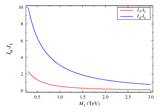
Plots of and as function of the leptoquark mass are shown in Fig. 2, for a fixed value of the vector-quark mass of 600 GeV.
To illustrate the range of parameters allowed by the neutrino mass, let us assume , so that only contribute to the neutrino mass matrix. If we further assume that only the the top quark (among ) mixes significantly with the vector-like quark, i.e., , then . Therefore, we can write
| (55) |
For normal neutrino mass hierarchy, is needed, which in turn requires . This means that for order one values of the Yukawa couplings , the mass of the vector-like quark and/or the leptoquarks is of order GeV. Conversely, if both the LQ and vector-like quark have masses of order TeV, and if , one must have . In both regimes, lepton flavor violation processes do not strongly constrain the model parameters. Interesting new effects will arise, however, if the vector-like quark/leptoquark masses are near a TeV, and if some of the Yukawa couplings lie in the range , as will be discussed in the next section.
Although the model predicts the lightest neutrino to be essentially massless, owing to the highly suppressed determinant of , Eq. (53) does admit both the normal hierarchy (NH) and the inverted hierarchy (IH) of neutrino masses. Since the off-diagonal elements of are uniquely related to the diagonal elements, one can determine the values of for as
| (56) |
where are obtained from
| (57) |
Here is the leptonic mixing matrix parameterized as in Ref. [20], while is given by
| (58) |
Take for example the ratio . Its value can be determined from Eq. (56), but this must match the product , also obtained from the same equation. Now, by using the central values of the current neutrino oscillation data, , , , , and the upper limit on , [21], one can find the allowed values of . This result is plotted in Fig. 3 versus , both for NH (upper left panel) and for IH (upper right panel). From this figure we see that the ratio of has to be of order one for normal hierarchy, while it can range from 0.5 to 1000 for inverted hierarchy. In both cases, the value of is allowed to range from zero up to the current upper limit. Recently, the T2K experiment [22] has reported an indication of nonzero , with the best fit value (assuming and ) being for normal (inverted) hierarchy. MINOS experiment also finds supporting evidence, although with less significance [23]. The present model can accommodate these indications for a sizable .


The couplings will mediate decays (see the next section for detailed discussions). One has for the ratio of branching ratios,
| (59) |
where [20]. Eq. (59) has an interesting consequence. As explained above, in the NH case, . This means the branching ratio of cannot exceed because of the limit on the branching ratio [25]. A measurement of near the current experimental limit of would rule out the NH scenario. Of course, for these decays to have significant branching ratios, the leptoquarks must have masses not much above a TeV. In Fig. 3, we also show the ratio as a function of allowed in the model for the NH case (lower left panel) and IH case (lower right panel). The ratio in our model, which can server as a further test.
3 Experimental constraints
The new interactions shown in Eqs. (5) and (30) can induce lepton flavor violation processes such as and decays. In this section we analyze various such processes and derive limits on model parameters. LHC experiments have set lower limits on the leptoquark mass: GeV for the first generation leptoquarks and GeV for the second generation leptoquarks, assuming branching ratio of 1(0.5) [24]. Our fit to neutrino mass suggests that the branching ratio of the leptoquark to muons is about 0.5, so we shall adopt the corresponding limits in this section.
3.1
This process occurs in the model via the one loop diagrams shown in Fig. 4. There are two couplings which are responsible for this process: and . In fact, the predictions of this model are similar to the ones discussed in Ref. [12], with one difference that here we have interference between diagrams generated by and those induced by . In the present model, ignoring the electron mass, which is an excellent approximation, the branching ratio is given by
| (60) |
where and . The dimensionless functions and are given by [26, 27]
| (61) |
The branching ratios for other processes can be derived in a similar way. The resulting constraints on the model parameters are summarized in Table 1. Here all of the experimental limits are taken from Ref. [20] except for limit which is taken from Ref. [25].

An interesting feature of this analysis is that the couplings are only weakly constrained from these processes. This is owing to a GIM–like cancelation for the amplitude for this process from the first two diagrams of Fig. 4. This is similar to the model discussed in Ref. [12]. This cancelation occurs, in the limit of down quark mass being zero, since the charge of the internal leptoquark () is twice as large and opposite in sign compared to the charge of of the internal down quark (. The amplitude for the diagram when the photon is emitted from the scalar line is twice smaller compared to the diagram where it is emitted from the fermion line, which leads to the cancelation. The amplitude that survives has a suppression of , which causes the weak limit. Because of this cancelation, we can derive correlated limits on the masses of the leptoquarks and the vector-like quark from , since only the couplings are involved. This is shown as a contour plot in Fig. 5. To get the largest possible masses, we set the Yukawa couplings , as large as allowed by perturbativity. If is discovered at the current limit [25] the masses should lie to the left of the red contour in Fig. 5, while a measurement of would require the masses to lie to the left of the blue contour. The LHC reach for a leptoquark of this type is 1.5 TeV [28], which would serve as a cross check in this case.
| Process | BR limit | Constraint | |
|---|---|---|---|

3.2
In this process, the photon can be off-shell, and therefore, there is no GIM-like cancelation for the contributions. It turns out that in addition to the photon penguin diagrams, there are also penguin diagrams and box diagrams (the Higgs boson exchange is suppressed by the electron mass). The mixing between vector-like quark and SM chiral quarks also plays a role in this process. The expression for the decay width is rather lengthy, which we do not present for brevity, but it is similar to the one given in Ref. [12]. To simplify the problem in deriving the constraints, we assume that only the top quark mixes with the vector-like quark, or equivalently in Eq. (), where is the Wolfenstein parameter, while could be as large as 0.3, consistent with constraint from constraint [29]. For exchange (corresponding to down-type quark inside the loop), we assume that there is no accidental cancelation among the different couplings , and thus omit terms such as with . For degenerate leptoquark masses of 400 GeV, and for the vector-like quark mass set equal to 600 GeV, we obtain:
| (62) |
for . These limits are obtained by assuming that contributions from one type of coupling dominates at a time. While these limits are stringent, they do not pose any restriction on the neutrino masses and mixings. The decay may be within reach of next generation experiments, with the couplings lying in the range and the leptoquark mass around a TeV.
3.3 conversion in nuclei
Since this model features direct interactions of quark and lepton via the leptoquarks, conversion in nuclei occurs. The diagrams are similar to the ones discussed in Ref. [12], with tree level and loop contributions. There is a more direct link between neutrino mass and the loop induce conversion process. If we assume that only the top quark mixes with the vector-like quark as in the case of , then there is no tree level exchange contribution to this process. Following the procedure outlined in Ref. [12], from the limit on conversion in , we obtain (for GeV, and a vector-like quark mass of 600 GeV)
| (63) |
for . Again, this analysis suggests that for natural values of the model parameters, this process may be within reach of next generation experiments.

3.4 Tree level mixing
The FCNC that occurs in the up–quark sector (see Eq. (12)) induces tree level mixing mediated by the boson, as shown in Fig. 6. The neutral Higgs boson induced contribution from Eq. (13) is suppressed by light quark mass and can be ignored. The mixing amplitude is given by [30]
| (64) |
where is the meson mass, GeV is the meson decay constant, is the bag parameter, and is the QCD correction factor. All the numbers here are taken from Ref. [31]. By using GeV [20], one obtains the constraint
| (65) |
According to Eq. () this constraint implies . As a result of this limit, unlike in a four generation model where there is no such FCNC process, the vector–quark contributions to meson mixing (eg., in the sector) cannot be too large.
3.5 decay
Recently, the CDF collaboration has reported a hint for the decay , with [32]. LHCb collaboration has not confirmed such a hint, and quotes an upper limit [33]. The SM prediction for this branching ratio is , which means there is ample room for new physics in this process.
Tree level exchange of leptoquarks can contribute to decay in our model. The branching fraction is given by [34]
| (66) |
where the SM contributions have been ignored. This enables us to fit , with GeV for the leptoquark mass, and .
3.6 New CP violation in mixing
Our model of leptoquarks and vector-like quark generates new contributions to mixing. There are two sources, one through LQ induced box diagrams, and the other through SM-like box diagrams with the vector-like quark (see Fig. 7). Including these contributions, the mixing amplitude becomes
| (67) | |||||
The functions with are the Inami-Lim functions [35], whereas with are the QCD correction factors. The numerical values for these factors for a 600 GeV for vector-like quark mass are [36]
| (68) |

.
It is sometimes more convenient to parametrize as [37]
| (69) |
where and are the new contributions. With this parametrization, one can write
| (70) |
with , .
The main reason to highlight this phenomenon is because there are hints for new sources of CP violation beyond the SM in the DØ measurement inferred from the charge asymmetry in the same sign di-muon decay of the mesons [16]:
| (71) |
Here is the numbers of events containing two hadrons that decay semileptonically into two positive (negative) muons. Eq. (71) can be written as a linear combination of two asymmetries [38, 16]
| (72) |
where () is defined as [16]
| (73) |
In the SM, and [39], so that which is away from the current measurement (see Eq. (71)). A likely explanation is that there is a new source of CP violation in mixing.
Additionally, the measurements of relative phase between mixing amplitude and decay amplitude () as well as the measurements of decay width difference performed by CDF [40] and DØ [41] yield [42]:
| (74) |
Here there is a discrepancy from SM prediction for , which may be another hint for physics beyond the SM.
It is interesting to see whether the vector–like charge quark can resolve these problems. The best fit to the data for a fourth generation quarks, including the preferred values of the CKM mixing angles, is given in Ref. [43] which shows corresponding to which is still far from the experimental central value (see Eq. (74)). This result should hold in the present model as well. We conclude that the mixing with vector-like quark is not enough to get the central value of , so the LQ induced box diagram is a more promising source for the new physics here.
Ignoring the effect of extra family mixing, the LQ contribution , can satisfy the best fit given in Ref. [37], i.e. . This would correspond to where the index is summed. However, since the limits and must be satisfied, the dominant contribution should arise with the lepton inside the box diagram loop. The phase is not constrained and therefore can take the fitted value of .
3.7 versus

Analogous to the system, this model also provides new contributions to mixing, arising through LQ induced box diagrams and new mixing between SM quarks and the vector-like quark. Owing to the stringent constraint arising from the tree level mixing, see Eq. (65), analogous mixing in the system would be more suppressed. The new contributions to the mixing may explain the apparent discrepancy between and determinations within the SM. The fitted value of obtained from , , , , and measurements is given by
| (75) |
which differs by from the world average experimental value [42],
| (76) |
The three family SM fit to the various CKM observables is shown in Fig. 8. A possible explanation is that there is new physics that affects the system, which we parametrize as
| (77) |
where
| (78) | |||||
This is analogous to the discussion of mixing. With this formula, one can write
| (79) |
where
| (80) |
Unlike in the system, the effect of the vector-like quark can induce a significant effect to resolve the tension in determination. In order to see this effect, let us ignore for the moment the LQ contributions. Then, if we choose [43]
| (81) |
we obtain , which is in the good agreement with the experimental value. Note, that the LQ contribution is not strongly constrained by neutrino mass nor lepton flavor violation, so it can get close to the experimental value, as long as the LQ mass is less than 1 TeV.
3.8 Neutrinoless double beta decay
Although this model can accommodate inverted hierarchy in which neutrinoless double beta decay () may occur with sizable effect, it is still interesting to see that even in the normal hierarchy case, such process may be observed through vector-scalar exchange mechanism [18], depicted in Fig. 9.

The effective Lagrangian of the new vertex after Fierz rearrangement is
| (82) |
where
| (83) |
This process is similar to MSSM models without -parity violation discussed in [18] and [44]. Following Ref. [44], and by using the results from Heidelberg-Moscow experiment on decay rate [45], one obtains for GeV and GeV
| (84) |
The mixing matrix elements is constrained by mixing process and has to be less than . Since the coupling is not constrained by neutrino mass, it could be of order one. For and (assuming NH case and vector mass of order sub-TeV) from lepton flavor violation constraints, one ses that neutrinoless double beta decay might be observable even in the case of normal mass hierarchy. Of course, for this to be valid, the leptoquarks and vector-like quark have to be light.
4 Conclusions
In this paper we have presented a new two-loop neutrino mass generation model which has the effective operator of Eq. (2). Generating this effective operator in a renormalizable theory would require the addition of a charge 2/3 vector-like quark and a scalar leptoquark doublet tot the standard model spectrum. We have studied the phenomenology of this model. This model can explain the CP violation parameters in the and the system. The leptoquarks of the model generate new CP violating contributions in mixing, which can explain the di-muon anomaly reported by DØṪhe apparent tension in the determination of from decays and from the global analysis including from the meson system also finds a natural explanation in this model. Neutrinoless double beta decay may occur through vector-scalar exchange and may be observable even with a normal hierarchy in the neutrino masses.
Acknowledgement
This work is supported by in part the US Department of Energy, Grant Numbers DE-FG02-04ER41306.
References
- [1] S. Weinberg, Phys. Rev. Lett. 43, 1566 (1979).
- [2] P. Minkowski, Phys. Lett. B 67, 421 (1977); M. Gell-Mann, P. Ramond, and R. Slansky, in Supergravity, eds. D. Freedman et al., (North-Holland, Amsterdam, 1980); T. Yanagida, in Proceedings of the Workshop on Baryon Number in the Universe, eds. O. Sawada and A. Sugamoto, (KEK, 1979); R. Mohapatra and G. Senjanović, Phys. Rev. Lett. 44, 912 (1980).
- [3] A. Zee, Phys. Lett. B93, 389 (1980).
- [4] T. P. Cheng and L. -F. Li, Phys. Rev. D 22, 2860 (1980).
- [5] L. J. Hall and M. Suzuki, Nucl. Phys. B 231, 419 (1984).
- [6] A. Zee, Nucl. Phys. B 264, 99 (1986).
- [7] K. S. Babu, Phys. Lett. B203, 132 (1988).
- [8] K. S. Babu and C. N. Leung, Nucl. Phys. B 619, 667 (2001).
- [9] L. Wolfenstein, Nucl. Phys. B 175, 93 (1980).
- [10] Y. Koide, Phys. Rev. D 64, 077301 (2001); P. H. Frampton, M. C. Oh and T. Yoshikawa, Phys. Rev. D 65, 073014 (2002); X. G. He, Eur. Phys. J. C 34, 371 (2004).
- [11] K. S. Babu and C. Macesanu, Phys. Rev. D 67, 073010 (2003); M. Nebot, J. F. Oliver, D. Palao, and A. Santamaria, Phys. Rev. D 77, 093013 (2008); D. Aristizabal Sierra and M. Hirsch, JHEP 0612, 052 (2006).
- [12] K. S. Babu and J. Julio, Nucl. Phys. B 841, 130 (2010).
- [13] K. -w. Choi, K. S. Jeong and W. Y. Song, Phys. Rev. D 66, 093007 (2002).
- [14] A. de Gouvea and J. Jenkins, Phys. Rev. D 77, 013008 (2008).
- [15] For a recent analysis see: P. Dey, A. Kundu, B. Mukhopadhyaya and S. Nandi, JHEP 0812, 100 (2008).
- [16] V. M. Abazov et al. [D0 Collaboration], arXiv:1106.6308 [hep-ex].
- [17] E. Lunghi and A. Soni, Phys. Lett. B 697, 323 (2011); E. Lunghi and A. Soni, Phys. Lett. B 666, 162 (2008); E. Lunghi and A. Soni, arXiv:1104.2117 [hep-ph].
- [18] K. S. Babu and R. N. Mohapatra, Phys. Rev. Lett. 75, 2276 (1995).
- [19] H. Harari and M. Leurer, Phys. Lett. B 181, 123 (1986); H. Fritzsch and J. Plankl, Phys. Rev. D 35, 1732 (1987).
- [20] K. Nakamura et al. [Particle Data Group], J. Phys. G 37, 075021 (2010).
- [21] T. Schwetz, M. A. Tortola, and J. W. F. Valle, New J. Phys. 10, 113011 (2008); M. Mezzetto and T. Schwetz, J. Phys. G 37, 103001 (2010).
- [22] K. Abe et al. [T2K Collaboration], arXiv:1106.2822 [hep-ex].
- [23] P. Adamson et al. [MINOS Collaboration], Phys. Rev. Lett. 107, 181802 (2011).
- [24] G. Aad et al. [ATLAS Collaboration], Phys. Rev. D 83, 112006 (2011). [arXiv:1104.4481 [hep-ex]].
- [25] J. Adam et al. [MEG collaboration], arXiv:1107.5547 [hep-ex].
- [26] J. Hisano, T. Moroi, K. Tobe and M. Yamaguchi, Phys. Rev. D 53, 2442 (1996).
- [27] L. Lavoura, Eur. Phys. J. C 29, 191 (2003).
- [28] A. Belyaev, C. Leroy, R. Mehdiyev and A. Pukhov, JHEP 0509, 005 (2005).
- [29] J. Alwall et al., Eur. Phys. J. C 49, 791 (2007).
- [30] G. C. Branco, P. A. Parada and M. N. Rebelo, Phys. Rev. D 52, 4217 (1995); E. Golowich, J. Hewett, S. Pakvasa and A. A. Petrov, Phys. Rev. D 76, 095009 (2007).
- [31] M. Bona et al. [UTfit Collaboration], JHEP 0803, 049 (2008).
- [32] T. Aaltonen et al. [CDF Collaboration], arXiv:1107.2304 [hep-ex].
- [33] R. Aaij et al. [LHCb Collaboration], arXiv:1112.1600.
- [34] A. Dighe, A. Kundu and S. Nandi, Phys. Rev. D 82, 031502 (2010); A. Dighe, A. Kundu and S. Nandi, Phys. Rev. D 76, 054005 (2007).
- [35] T. Inami and C. S. Lim, Prog. Theor. Phys. 65, 297 (1981) [Erratum-ibid. 65, 1772 (1981)].
- [36] A. Soni, A. K. Alok, A. Giri, R. Mohanta and S. Nandi, Phys. Rev. D 82, 033009 (2010).
- [37] Z. Ligeti, M. Papucci, G. Perez and J. Zupan, Phys. Rev. Lett. 105, 131601 (2010).
- [38] Y. Grossman, Y. Nir and G. Raz, Phys. Rev. Lett. 97 (2006) 151801.
- [39] A. Lenz and U. Nierste, JHEP 0706, 072 (2007).
- [40] T. Aaltonen et al. [CDF Collaboration], Phys. Rev. Lett. 100, 161802 (2008).
- [41] V. M. Abazov et al. [D0 Collaboration], Phys. Rev. Lett. 101, 241801 (2008).
- [42] D. Asner et al. [Heavy Flavor Averaging Group], arXiv:1010.1589 [hep-ex].
- [43] A. K. Alok, A. Dighe and D. London, arXiv:1011.2634 [hep-ph].
- [44] H. Päs, M. Hirsch, and H. V. Klapdor-Kleingrothaus, Phys. Lett. B459, 450 (1999).
- [45] L. Baudis et al., Phys. Lett. B 407, 219 (1997).