A scalar field dark matter model and its role in the large scale structure formation in the universe
Abstract
In this work we present a model of dark matter based on scalar-tensor theory of gravity. With this scalar field dark matter model we study the non-linear evolution of the large scale structures in the universe. The equations that govern the evolution of the scale factor of the universe are derived together with the appropriate Newtonian equations to follow the non-linear evolution of the structures. Results are given in terms of the power spectrum that gives quantitative information on the large-scale structure formation. The initial conditions we have used are consistent with the so called concordance CDM model.
I Introduction
The standard model of cosmology is supported by three main astronomical observations: the surveys of supernovae Ia, the cosmic microwave background radiation (CMB), and the primordial nucleosynthesis. These observations together with other modern cosmological observations, like galaxies surveys (SDSS, 2dF), galaxy rotation curves, the Bullet Cluster observation, studies of clusters of galaxies, establish that the universe behaves as dominated by dark matter (DM) and dark energy. However, the direct evidence for the existence of these invisible components remains lacking. Several theories that would modify our understanding of gravity have been proposed in order to explain the large scale structure formation in the universe and the galactic dynamics. The best model we have to explain the observations is the CDM model, i.e., the model of cold dark matter (CDM) –non-relativistic particles of unknown origin– with cosmological constant (), in particular, this model explains very well the universe on scales of galaxy clusters and up [1].
The CDM model has become the theoretical paradigm leading the models of the universe to explain the large scale structure (LSS) formation and several other observations. Where “large” means scales larger than Mpc –about the size of the group of galaxies that our Milky Way belongs. Together with the cosmic inflation theory, this model makes a clear prediction about the necessary initial conditions that the universe has to have in order to have the structures we observe and that those structures build hierarchically due to a gravitational instability. One of its main predictions is that the density profile of galaxies, clusters of galaxies, and so on, is of the form [2, 3],
a density profile known as Navarro-Frenk-White profile (NFW). Parameters and must be fitted, for example, using rotation curves of galaxies.
The CDM model and its success in explaining several observations –this is why this model is also known as the concordance model– yields the following conclusions: On large scales, the universe is homogeneous and isotropic, as described by the Friedmann-Lamaître-Robertson-Walker (FLRW) metric. The geometry of the universe is flat, as predicted by inflation. The dark matter is cold (non-relativistic at decoupling epoch). The initial density fluctuations were small and described by a Gaussian random field. The initial power spectrum of the density fluctuations was approximately the Harrison-Zeldovich spectrum (, ) [5, 4].
In terms of the composition of the universe, the above conclusions can be summarized as follows: Hubble’s constant (Expansion rate of the universe at the present epoch): km/s/Mpc. Density parameter (combined mass density of all kind of mass and energy in the universe, divided by the critical density): . Matter density parameter (combined mass density of all forms of matter in the universe, divided by the critical density): . Ordinary matter parameter density (density of mass of ordinary atomic matter in the universe divided by the critical density): . Density parameter of dark energy (energy density of dark energy in the universe divided by the critical density): [6].
Even though of all successes of the CDM, this model has several problems. Some of them are: The exotic weakly interacting particles proposed as dark matter particles candidates are still undetected in the laboratory. The number of satellites in a galaxy such as the Milky Way is predicted to be an order of magnitude larger than is observed. Cuspy halo density profiles. The lack of evidence in the Milky Way for a major merger is hard to reconcile with the amount of accretion predicted by CDM. With respect to the inclusion of the cosmological constant, the ratio of the vacuum energy density to the radiation energy density after inflation is 1 part in , a fine tuning coincidence. The cosmological constant has the wrong sing according to the string theorists who prefer a negative instead of a positive . The CDM model predicts that large structures should form last and therefore should be young whereas observations tell us that the largest galaxies and clusters appear old. Several candidates have been proposed in the past that pretend to substitute the role that the cosmological constant plays to accelerate the expansion of the universe. That the universe is expanding is supported mainly by the observations of the supernova project SNIa[7, 8]. And we have lead to conclude that the universe is now dominated by an energy density with negative pressure and occupies about 70% of the universe in the present epoch. This energy is called generically the dark energy. Several models to explain this dark component has been proposed, and they may be classified accordingly to its equations of state as the following: quintessence dark energy[9, 10], phantom energy [11, 12], or the quintom cosmology paradigm[13] (see also the review[14] for even more details). Cosmological constant has as its equation of state one in which the pressure is the negative of the density.
From the -body numerical simulations point of view we have two works, in which a detailed analysis of two scalar field possibilities has been explored. One is the coupled quintessence models [15] and the other is the extended quintessence models [16]. The former considers a scalar field coupled minimally to the Ricci scalar and is coupled to the Lagrangian matter contribution. The later is of the type of a scalar-tensor theory in which the scalar field is introduced to model dark energy with a potential that is an inverse power law. The model we present in this work pretends to model the dark matter contribution in the large scale structure formation with a scalar field model that stems from the newtonian limit of a general scalar-tensor theory [17].
Another problem that the CDM problem is facing is the following. Almost a decade ago a bow shock in the merging cluster 1E0657-56, known as the Bullet Cluster, observed by satellite Chandra indicates that the subcluster –found by [18]– moving through this massive ( M⊙) main cluster creates a shock with a velocity as high as 4700 km s-1 [19, 20]. A significant offset between the distribution of X-ray emission and the mass distribution has been observed [21, 22], also indicating a high-velocity merger with gas stripped by ram pressure. Several authors have done detailed numerical non-cosmological simulations [26, 27, 24, 25, 23]. One of the key input parameters for the simulations is to set the initial velocity of the subcluster, which is usually given at somewhere near the virial radius of the main cluster. [28] have run cosmological N-body simulation using a large box (27 Gpc3) to calculate the distribution of infall velocities of subclusters around massive main clusters. The infall velocity distribution were given at 1–3 –similar to the virial radius– and thus it gives the distribution of realistic initial velocities of subclusters just before collision. This distribution of infall velocities must be compared with the best initial velocity used by [23] of 3000 km s-1 at about to be in agreement with observations. [28] have found that such a high infall velocity is incompatible with the prediction of the CDM.
Therefore, there are plenty of problems that the concordance model have to solve and finally, it does not tell us what is dark matter and dark energy.
The program to study the large scale structure formation should be to start with primordial initial conditions which means give the initial relevant fields, such as for example, density and velocity fields at the epoch of last scattering (, the value of the redshift at that epoch, i.e., a photon emitted at that epoch is redshifted as , with the wavelength of the photon when emitted, and is the wavelength of the same photon when observed; the expansion factor for a universe with a flat geometry is related to the redshift as ). Then, evolve this initial condition using an -body scheme up to the present epoch ().
Some questions we have to answer are: What are the distribution of the LSS sizes? What is the amount of mass and its distribution at large scales? How are the voids distributed through the space? Are these voids devoid of any matter? How the LSS evolve with time? What is the DM equation of state? What is its role in the LSS formation processes and galactic dynamics? What are the implications of the observed LSS on the cosmological model of our universe? And on the structure formation? And of course, what is the nature of the dark energy and matter?
During the last decades there have been several proposals to explain DM, for example: Massive Compact Halo Objects (Machos), Weakly Interacting Massive Particles (WIMPs) such as supersymmetric particle like the neutralino. Other models propose that there is no dark matter and use general relativity with an appropriate equation of state. Or we can use scalar fields, minimally or non minimally coupled to the geometry.
In this work we are mainly concern with the problem of dark matter and its consequences on the large scale structure formation process. Our DM model is based on using a scalar field (SF) that is coupled non-minimally to the metric through the Ricci scalar in the Einstein field equations. A scalar field is the most simple field of nature. Nordstrom proposed a gravity theory by 1912, before Einstein [29]. Scalar fields have been around for so many years since pioneering work of Jordan, Brans, and Dicke. Nowadays, they are considered as: (a) inflation mechanism; (b) the dark matter component of galaxies; (c) the quintessence field to explain dark energy; and so on. Therefore, is natural to consider dark matter models based on modifications of Einstein’s general relativity that include scalar fields. In this paper we will show results about the role this scalar field plays on the non-linear large scale structure formation of the universe. In particular, we will show how the power spectrums predicted by this model compare with the power spectrums predicted by CDM and the ones that come from observations.
So we organize our work in the following form: In the next section we present the general theory of a typical scalar-tensor theory (STT), i. e., a theory that generalizes Einstein’s general relativity by including the contribution of a scalar field that couples non-minimally to the Ricci scalar. In section III we show how the Friedmann equations becomes within a STT and present our model for the evolution of the universe expansion factor . In section IV we present the -body method which we will use to obtain the evolution of the large scale structures. Our results for an initial condition of the fields that is consistent with the observations are given in section V. Finally, our conclusions are given in section VI.
II General scalar-tensor theory and its Newtonian limit
The Lagrangian that gives us the Einstein equations of general relativity is
| (1) |
The Einstein field equations that are obtained from the above Lagrangian, in the limit of small velocities as compared with the speed of light and small forces, limit known as the Newtonian limit, give us the standard Newtonian potential due to a point particle of mass
| (2) |
where is the gravitational constant. What we intend to do in this work is to obtain the consequences in the LSS formation processes when we rise the constant to a scalar field, . But we go beyond this approach and include in the Lagrangian two additional terms that depend on this field, a kinetic and potential terms. We will show, in particular, that the Newtonian limit of this theory gives for the Newtonian potential due to a mass [30],
| (3) |
i. e., the standard Newtonian potential is modified by an additional term that has the form of a Yukawa potential.
Then, we start with the Lagrangian of a general scalar-tensor theory
| (4) |
Here is the metric, is the matter Lagrangian and and are arbitrary functions of the scalar field. The fact that we have a potential term tells us that we are dealing with a massive scalar field. Also, the first term in the brackets, , is the one that gives the name of non-minimally coupled scalar field.
When we make the variations of the action, , with respect to the metric and the scalar field we obtain the Einstein field equations [29]
| (5) | |||||
for the metric and for the massive SF we have
| (6) |
where . Here is the energy-momentum tensor with trace , and are in general arbitrary functions that govern kinetic and potential contribution of the SF. If in Lagrangian (4) we set we get the Bergmann-Wagoner theory. If we further set the Jordan-Brans-Dicke theory is recovered. The gravitational constant is now contained in . Also, the potential contribution, , provides mass to the SF, denoted here by .
II.1 Newtonian limit of a STT
The study of large-scale structure formation in the universe is greatly simplified by the fact that a limiting approximation of general relativity, the Newtonian mechanics, applies in a region small compared to the Hubble length ( Mpc, where is the speed of light, km/s/Mpc, is Hubble’s constant and ), and large compared to the Schwarzschild radii of any collapsed objects. The rest of the universe affect the region only through a tidal field. The length scale is of the order of the largest scales currently accessible in cosmological observations and yr characterizes the evolutionary time scale of the universe [31].
Therefore, in the present study, we need to consider the influence of SF in the limit of a static STT, and then we need to describe the theory in its Newtonian approximation, that is, where gravity and the SF are weak (and time independent) and velocities of dark matter particles are non-relativistic. We expect to have small deviations of the SF around the background field, defined here as and can be understood as the scalar field beyond all matter. Accordingly we assume that the SF oscillates around the constant background field
and
where is the Minkowski metric. Then, Newtonian approximation gives [33, 34, 32, 30]
| (7) | |||||
| (8) |
we have set and . In the above expansion we have set the cosmological constant term equal to zero, since on small galactic scales its influence should be negligible. However, at cosmological scales we do take into account the cosmological constant contribution, see below.
Note that equation (7) can be cast as a Poisson equation for ,
| (9) |
and the New Newtonian potential is given by . Above equation together with
| (10) |
form a Poisson-Helmholtz equation and gives
which represents the Newtonian limit of the STT with arbitrary potential and function that where Taylor expanded around . The resulting equations are then distinguished by the constants , , and . Here is Planck’s constant.
The next step is to find solutions for this new Newtonian potential given a density profile, that is, to find the so–called potential–density pairs. General solutions to Eqs. (9) and (10) can be found in terms of the corresponding Green functions, and the new Newtonian potential is [30, 35]
| (11) | |||||
The first term of Eq. (11), is the contribution of the usual Newtonian gravitation (without SF), while information about the SF is contained in the second term, that is, arising from the influence function determined by the modified Helmholtz Green function, where the coupling () enters as part of a source factor.
The potential of a single particle of mass can be easily obtained from (11) and is given by
| (12) |
For local scales, , deviations from the Newtonian theory are exponentially suppressed, and for the Newtonian constant diminishes (augments) to for positive (negative) . This means that equation (12) fulfills all local tests of the Newtonian dynamics, and it is only constrained by experiments or tests on scales larger than –or of the order of– , which in our case is of the order of galactic scales. In contrast, the potential in the form of equation (3) with the gravitational constant defined as usual does not fulfills the local tests of the Newtonian dynamics [36].
It is appropriate to give some additional details on the Newtonian limit for the Einstein equations without scalar fields (see [31]). We are considering a small region compared to the Hubble length but large compared to the Schwarzschild radii of any collapsed object. In this small region the metric tensor was written as where is small as compared to the Minkowski metric . In this region Einstein’s field equations are simple because the standard weak field linear approximation applies. One finds,
| (13) | |||||
| (14) |
Then, the zero-zero component of the field equations for an ideal fluid with density , pressure , and velocity becomes
| (15) |
For completeness the cosmological constant has been added. The geodesic equations, in the limit , , are
| (16) |
Equations (15) and (16) are the standard equations of Newtonian mechanics, except that if there is an appreciable radiation background, one must take into account the active gravitational mass associated with the pressure, and of course if , there is the cosmic force between particles at separation r.
Equations (15) and (16) apply to any observer outside a singularity, though depending on the situation, the region within which these equations apply need not contain much matter. The region can be extended by giving the observer an acceleration to bring the observer to rest relative to distant matter, which adds the term to , and then by patching together the results from neighboring observers. This works (the acceleration and potentials can be added) as long as relative velocities of observers and observed matter are and (equation (14)). For a region of size containing mass with density roughly uniform, this second condition is
| (17) |
In the Friedmann-Lemaître models Hubble’s constant is
| (18) |
If one assumes is negligible and the density parameter , so equation (17) indicates
| (19) |
That is, the region must be small compared to the Hubble length. Since the expansion velocity is , this condition also says .
The Newtonian approximation can fail at much smaller if the region includes a compact object like a neutron star or black hole, but one can deal with this by noting that at distances large compared to the Schwarzschild radius the object acts like an ordinary Newtonian point mass. It is speculated that in nuclei of galaxies there might be black holes as massive as M⊙, Schwarzschild radius cm. If this is an upper limit, Newtonian mechanics is a good approximation over a substantial range of scales, .
II.2 Multipole expansion of the Poisson-Helmholtz equations
The Poisson’s Green function can be expanded in terms of the spherical harmonics, ,
where is the smaller of and , and is the larger of and and it allows us that the standard gravitational potential due to a distribution of mass , without considering the boundary condition, can be written as [37]
where () are the internal (external) multipole expansion of ,
Here, the coefficients of the expansions and , known as internal and external multipoles, respectively, are given by
The integrals are done in a region where for the internal multipoles and in a region where for the external multipoles. They have the property
We may write expansions above in cartesian coordinates up to quadrupoles. For the internal multipole expansion we have
| (23) |
and its force is
| (24) |
where
| (25) |
| (26) |
| (27) |
For the external multipoles we have
| (28) |
and its force is
| (29) | |||||
where
| (30) |
| (31) |
| (32) |
The external multipoles have the usual meaning, i.e., is the mass, is the dipole moment, and is the traceless quadrupole tensor, of the volume . We may atach to the internal multipoles similar meaning, i.e., is the internal “mass”, is the internal “dipole” moment, and is the traceless internal “quadrupole” tensor, of the volume .
In the case of the scalar field, with the expansion
the contribution of the scalar field to the Newtonian gravitational potential can be written as
where, for simplicity of notation, we are using and
and are the modified spherical Bessel functions.
We have defined the multipoles for the scalar field as
They, also, have the property
The above expansions of SF contribution to the Newtonian potential can be written in cartesian coordinates. The internal multipole expansion of the SF contribution, up to quadrupoles is
| (36) | |||||
and its force is
| (37) | |||||
where
| (38) |
| (39) |
| (40) |
In the exterior region the SF multipole contribution to the potential is
| (41) | |||||
and its force is
| (42) | |||||
where
| (43) |
| (44) |
| (45) |
In the limit when we recover the standard Newtonian potential and force expressions.
Up to here the formulation is general, i.e., mass distribution may have any symmetry or none at all. In order to take advantage of the symmetry of the spherical harmonics, the mass distribution must be spherically symmetric.
III Cosmological evolution equations using a static STT
To simulate cosmological systems, the expansion of the universe has to be taken into account. Also, to determine the nature of the cosmological model we need to determine the composition of the universe, i. e., we need to give the values of , with , for each component , taking into account in this way all forms of energy densities that exist at present. If a particular kind of energy density is described by an equation of state of the form , where is the pressure and is a constant, then the equation for energy conservation in an expanding background, , can be integrated to give .
Then, the Friedmann equation for the expansion factor is written as
| (46) |
where characterizes equation of state of species .
The most familiar forms of energy densities are those due to pressureless matter with (that is, nonrelativistic matter with rest-mass-energy density dominating over the kinetic-energy density ) and radiation with . The density parameter contributed today by visible, nonrelativistic, baryonic matter in the universe is and the density parameter that is due to radiation is .
In this work we will consider a model with only two energy density contribution. One which is a pressureless and nonbaryonic dark matter with that does not couple with radiation. Although in the numerical simulations we may include in the baryonic matter. Other, that will be a cosmological constant contribution with and equation of state . The above equation for becomes
| (47) |
The above discussion gives us the standard cosmological model with cosmological constant, i. e., CDM model.
In the framework of a scalar-tensor theory the cosmology is given as follows. If we use the Friedmann metric [29]
| (48) |
in the time-time component of the Einstein field equations (Hamiltonian constraint) gives
| (49) |
while the equation for the scalar field is
| (50) |
and the equation of the fluid is
| (51) |
The cosmological evolution of the initial perturbed fields should be computed using the above equations for the expansion factor. However, here, we will employ a cosmological model with a static SF which is consistent with the Newtonian limit given above. Thus, the scale factor, , is given by the following Friedman model,
| (52) |
where , and are the matter and energy density evaluated at present, respectively. The denominator appears in Eq. (52) due to the fact that we have defined and . Then, whenever appears the gravitational constant , we replaces it by .
We notice that the source of the cosmic evolution is deviated by the term when compared to the standard Friedmann-Lemaître model. Therefore, it is convenient to define a new density parameter by . This new density parameter is such that , which implies a flat universe, and this shall be assumed in the following computations, where we consider .
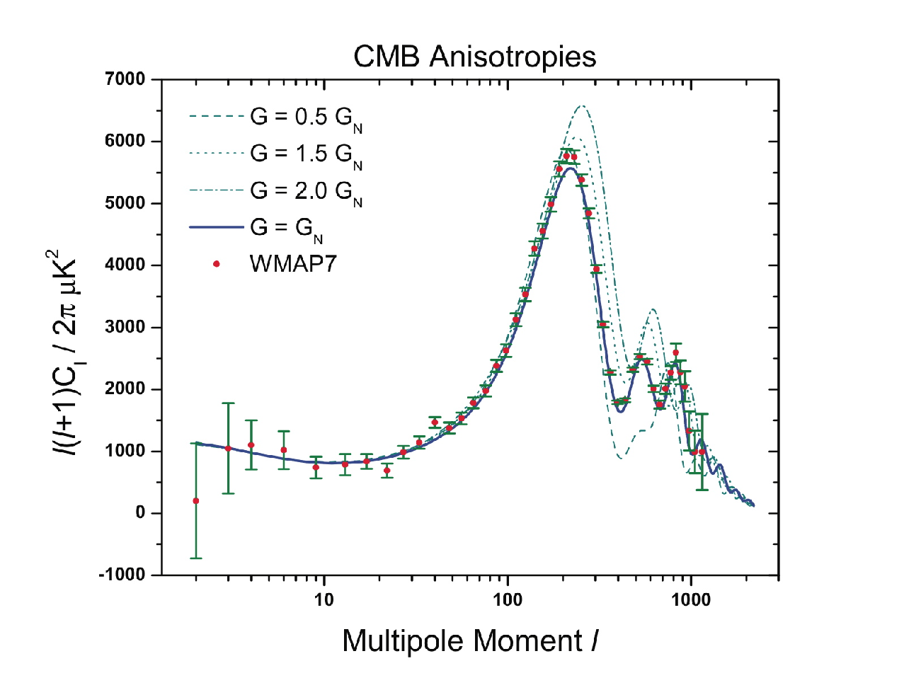
For positive values of , a flat cosmological model demands to have a factor more energy content ( and ) than in standard cosmology. On the other hand, for negative values of one needs a factor less and to have a flat universe. To be consistent with the CMB spectrum and structure formation numerical experiments, cosmological constraints must be applied on in order for it to be within the range [38, 39, 40, 41]. In figure 1 we show the effect of different values of the gravitational constant on the anisotripies of the CMB.
IV Vlasov-Poisson-Helmholtz equations and the -body method
The Vlasov-Poisson equation in an expanding universe describes the evolution of the six-dimensional, one-particle distribution function, . The Vlasov equation is given by,
| (53) |
where is the comoving coordinate, , is the particle mass, and is the self-consistent gravitational potential given by the Poisson equation,
| (54) |
where is the background mass density. The Vlasov-Poisson system, Eqs. (57) and (54) form the Vlasov-Poisson equation, constitutes a collisionless, mean-field approximation to the evolution of the full -body distribution.
An -body code attempts to solve the Vlasov-Poisson system of equations by representing the one-particle distribution function as
| (55) |
Substitution of (55) in the Vlasov-Poisson system of equations yields the exact Newton’s equations for a system of gravitating particles (See [43] for details),
| (56) |
where the sum includes all periodic images of particle and numerically is done using the Ewald method, see [44]. It is important to keep in mind, however, that we are not really interested in solving the exact -body problem for a finite number of particles, . The actual problem of interest is the exact -body problem in the fluid limit, i. e., as . For this reason, one important aspect of the numerical fidelity of -body codes lies in controlling errors due to the discrete nature of the particle representation of .
In the Newtonian limit of STT of gravity to describe the evolution of the six-dimensional, one-particle distribution function, we need to solve the Vlasov-Poisson-Helmholtz equation in an expanding universe [45, 46, 47, 48, 49]. The Vlasov equation is given by
| (57) |
where with satisfying Poisson equation
| (58) |
and satisfying the Helmholtz equation
| (59) |
Above equations form the Vlasov-Poisson-Helmholtz system of equations, constitutes a collisionless, mean-field approximation to the evolution of the full -body distribution in the framework of the Newtonian limit of a scalar-tensor theory.
Using the representation of the one-particle distribution function (55) the Newtonian motion equation for a particle , is written as [46]
| (60) | |||||
where the sum includes all periodic images of particle , and is
| (61) |
which, for small distances compared to , is and, for long distances, is , as in Newtonian physics.
The function is shown in Fig. 2 for several values of parameter . The horizontal line at is for the standard Newtonian case (). The long dash line above the horizontal standard line is for , the medium dash line is for and the tiny dash line is for . For negative values of the lines are below the standard horizontal case. Long dash line is for and medium dash line is for . We should notice that even though Mpc, gives an important contribution to the force between particles for .

V Results
In this section, we present results of cosmological simulations of a CDM universe with and without SF contribution in order to study the large scale structure formation.
We have used the standard Zel’dovich approximation [5] to provide the initial particles displacement off a uniform grid and to assign their initial velocities in a Mpc box[50]. In this approximation the comoving and the lagrangian coordinates are related by
| (62) | |||||
| (63) |
where the displacement vector is related to the velocity potential and the power spectrum of fluctuations :
| (64) | |||||
| (65) |
where and are gaussian random numbers with the mean zero and dispersion ,
| (66) |
where is a gaussian number with mean zero and dispersion 1.
The parameter together with the power spectrum , define the normalization of the fluctuations. The initial power spectrum was generated using the fitting formula by [51] for the transfer function. This formula is a slight variation of the common BBKS fit [52].
Therefore, for the standard CDM we have for the initial condition that the starting redshift is and we choose the following cosmology: (where includes cold dark matter and baryons), , , km/s/Mpc, , and . Particle masses are in the order of M⊙. The individual softening length was 50 kpc. This choice of softening length is consistent with the mass resolution set by the number of particles. All these values are in concordance with measurements of cosmological parameters derived from the seven-year data of the WMAP [6]. The initial condition –called the big box case– is in the Cosmic Data Bank web page: (http://t8web.lanl.gov/people/heitmann/test3.html). See [50] for more details.
Because the visible component is the smaller one and given our interest to test the consequences of including a SF contribution to the evolution equations, our model excludes gas particles, but all its mass has been added to the dark matter. We restrict the values of to the interval (see [38, 39, 40, 41]) and use Mpc, since these values sweep the scale lengths present in the simulations.
In all the simulations we have done, with or without the scalar field contribution, we demand that the cosmological model be flat. In this model with a scalar field a flat universe is obtained if , with and . Then, for positive values of we need a factor more energy content ( and ) that in the standard cosmology. Whereas for negative values of we need a factor of less and to have a flat universe. With this recipe and for a given value of we modified the above CDM initial condition accordingly.


In Fig. 3 we show how the above initial conditions evolve and give us the LSS formation process without SF and with SF. In (a) without SF. In (b) with SF: and Mpc. In (c) with SF: and Mpc. In (d) with SF: and Mpc. In (e) with SF: and Mpc. In (f) With SF: and Mpc. In (g) With SF: and Mpc.
To study the structure formation in the universe we follow the evolution of the overdensity [4],
where is the average density over a volume and is the comoving distance related to the physical density by . In the linear regime .
The correlation function tell us how is correlated in two nearby points and ,
and the power spectrum is the Fourier transform of the correlation function,
In Fig. 4 (a) we show the evolution of the power spectrum for the big box Mpc without SF, for several values of the redshift . We have used the POWMES code to compute the matter power spectrum [53]. In this figure we can appreciate how it is forming structures, upper curve of the power spectrum for the present epoch, . Fig. 4 (b) shows the power spectrum for the same values as in Fig. 3. Continuous line is without SF. Upper curve (dashed line) is with SF: and Mpc. Lower curve (dashed-dotted line) is with SF: and Mpc. The curve that is just below the continuous line (dotted line) is with SF: and Mpc. More greater values of the power spectrum means more structure formation. Therefore, the inclusion of a SF modifies the structure formation process. Depending of the values of its parameters, and we can obtain more structure or less structure at the present epoch, .


In our results as shown in Figs. 3 (c), (f) and (g), and 4 we have used a fix value of Mpc. For a given the role of SF parameter on the structure formation can be inferred by looking at equations (60) and (61) and Fig. 2 where we show the behavior of as a function of distance for several values of . The factor augments (diminishes) for positive (negative) values of for small distances compared to , resulting in more (less) structure formation for positive (negative) values of compared to the CDM model. In the case of the upper curve in Fig. 4 (b), for , the effective gravitational pull has been augmented by a factor of 2, in contrast to the case shown with the lower line in Fig. 4 (b) where it has been diminished by a factor of 1/2. That is why we observe for more structure formation in the case of the upper curve in Fig. 4 (b) and lesser in the case of the lower curve in the same figure. The effect is then, for a increasing positive , to speed up the growth of perturbations, then the halos, and then the clusters, whereas negative values of tend to slow down the growth. We also observe that for the large scale regimen of our simulations ( Mpc) they tend to predict almost the same structure formation. From comparison with the experimental results, we see that the CDM agrees well with SDSS observations, but predicts more structure formation than observations show in the Lyman- forest power spectrum. In general the more favored model is the model with SF with and Mpc.
VI Conclusions and final comments
We have used a general, static STT, that is compatible with local observations by the appropriate definition of the background field constant, i. e., , to study the LSS formation process. The initial condition for the several cases (different values of parameter ) was built in such a way that the geometry of the model universe were flat. Quantitatively, this demands that our models have and this changes the amount of dark matter and energy of the models in order to have a flat cosmology.
Using the resulting modified dynamical equations, we have studied the LSS formation process of a CDM universe. We varied the amplitude and sign of the strength of the SF (parameter ) in the interval and performed several 3D-simulations with the same initial conditions. From our simulations we have found that the inclusion of the SF changes the local dynamical properties of the most massive groups, however, the overall structure is very similar, as can be seen in Fig. 3.
The general gravitational effect is that the interaction between dark matter particles given by the potential (see equation (12)) changes by a factor , equation (61), in comparison with the purely Newtonian case. Thus, for the growth of structures speeds up in comparison with the Newtonian case (without SF). For the case the effect is to diminish the formation of structures.
It is important to note that particles in our model are gravitating particles and that the SF acts as a mechanism that modifies gravity. The effective mass of the SF () only sets an interaction length scale for the Yukawa term.
In this work we only varied the amplitude of the SF –parameter – leaving the scale length, , of the SF unchanged. However, in other studies we have done [48] we have found that increasing enhances the structure formation process for positive, and decreasing makes the structures grow at a slower rate.
We have computed the mass power spectrum in order to study the LSS formation process. The theoretical scheme we have used is compatible with local observations because we have defined the background field constant or equivalently that the local gravitational constant is given by , instead of being given by . A direct consequence of the approach is that the amount of matter (energy) has to be increased for positive values of and diminished for negative values of with respect to the standard CDM model in order to have a flat cosmological model. Quantitatively, our model demands to have and this changes the amount of dark matter and energy of the model for a flat cosmological model, as assumed. The general gravitational effect is that the interaction including the SF changes by a factor for in comparison with the Newtonian case. Thus, for the growth of structures speeds up in comparison with the Newtonian case. For the case the effect is to diminish the formation of structures. For the dynamics is essentially Newtonian.
Comparison with the power spectrums from galaxies in the SDSS catalog and that inferred from Lyman- forest observations tell us that CDM predicts more structure formation in the regime of smaller scales ( Mpc). Whereas, the model with SF with and Mpc, follows the general trend of the observed power spectrum. In this way we are able to construct a model that predicts the observed structure formation in the regime of small scales, with lesser number of halo satellites than the CDM model.
References
- [1] N. Bretón, J.L. Cervantes-Cota, and M. Salgado (Editors), The Early Universe and Observational Cosmology. (Springer-Verlag, Berlin Heidelberg, 2004).
- [2] J.F. Navarro, et al., Astrophys. J. 462, 563 (1996).
- [3] J.F. Navarro, et al., Astrophys. J. 490, 493 (1997).
- [4] J. Binney and S. Tremaine, Galactic Dynamics, Second Edition. (Princeton University Press, Princeton, 2008).
- [5] Y.B. Zel’dovich, Astron. & Astrophys. 5, 84 (1970).
- [6] E. Komatsu et al., Astrophys. J. Suppl. 192, 18 (2011). arXiv:1001.4538.
- [7] A.G. Riess, et al., Astron. J. 116, 1009 (1998). arXiv:astro-ph/9805201.
- [8] S. Perlmutter, et al., Astrophys. J. 517, 565 (1999). arXiv:astro-ph/9812133.
- [9] B. Ratra, P.J.E. Peebles, Phys. Rev. D 37, 3406 (1988).
- [10] C. Wetterich, Nuclear Phys. B 302, 668 (1988).
- [11] R.R. Caldwell, Phys. Lett. B 545, 23 (2002).
- [12] R.R. Caldwell, M. Kamonkowski, N.N. Weinberg, Phys. Rev. Lett. 91, 071301 (2003).
- [13] B. Feng, X.L. Wang, X.M. Zhang, Phys. Lett. B 607, 35 (2005).
- [14] Yi-Fu Cai, E.N. Saridakis, M.R. Setare, Jun-Qing Xia, Phys. Rep. 493, 1 (2010).
- [15] B. Li, J.D. Barrow, Phys. Rev. D 83, 024007 (2011).
- [16] B. Li, D.F. Mota, J.D. Barrow, Astrophys. J. 728, 109 (2011).
- [17] M. A. Rodríguez-Meza, J. Klapp, J.L. Cervantes-Cota, and H. Dehnen in Exact solutions and scalar fields in gravity: Recent developments, Edited by A. Macias, J.L. Cervantes-Cota, and C. Lämmerzahl, Kluwer Academic/Plenum Publishers, NY, 2001, p. 213. arXiv:0907.2466 [astro-ph.CO].
- [18] R. Barrena, A. Biviano, M. Ramella, E.E. Falco, and S. Steitz Astron. & Astrophys. 386, 816 (2002).
- [19] M. Markevitch, A.H. Gonzalez, L. David, A. Vikhlinin, S. Murray, W. Forman, C. Jones, W. Tucker, Astrophys. J. 567, L27 (2002).
- [20] M. Markevitch in Pro. X-Ray Universe 2005, Wilson (editor). (ESA SP-604; Noordwijk:ESA, 2006). pp. 723.
- [21] D. Clowe, et al., ApJ, 604, 596 (2004).
- [22] D. Clowe, et al., ApJ, 648, L109 (2006).
- [23] C. Mastropietro, and A. Burkert Mon. Not. R. Astron. Soc. 389, 967 (2008).
- [24] M. Milosavljevic, et al., Astrophys. J. 661, L131 (2007).
- [25] V. Springel and G. Farrar Mon. Not. R. Astro. Soc. 380, 911 (2007).
- [26] M. Takizawa, Astrophys. J. 629, 791 (2005).
- [27] M. Takizawa, PASJ, 58, 925 (2006).
- [28] L. Lee and E. Komatsu, Astrophys. J. 718, 60 (2010). arXiv:1003.0939
- [29] V. Faraoni, Cosmology in Scalar-Tensor Gravity. (Kluwer Academic Publishers, Dordrecht, The Netherlands, 2004).
- [30] M.A. Rodríguez-Meza and J.L. Cervantes-Cota Mon. Not. R. Astron. Soc. 350, 671 (2004).
- [31] P.J.E. Peebles The Large-Scale Structure of the Universe. (Princeton University Press, Princeton, 1980).
- [32] T. Helbig, Astrophys. J. 382, 223 (1991).
- [33] L.O. Pimentel and O. Obregón, Astrophysics and Space Science, 126, 231 (1986).
- [34] M. Salgado, arXiv: gr-qc/0202082 (2002).
- [35] M.A. Rodríguez-Meza, J.L. Cervantes-Cota, M.I. Pedraza, J.F. Tlapanco, and E.M. De la Calleja, Gen. Rel. Grav., 37, 823 (2005).
- [36] E. Fischbach and C.L. Talmadge, The Search for Non-Newtonian Gravity. (Springer-Verlag, New York, 1999).
- [37] J.D. Jackson, Classical Electrodynamics, Second Edition. (John Wiley & Sons, Inc., New York, 1975).
- [38] R. Nagata, T. Chiba, N. Sugiyama Phys. Rev. D 66, 103510 (2002).
- [39] R. Nagata, T. Chiba, N. Sugiyama Phys. Rev. D 69, 083512 (2004).
- [40] A. Shirata, T. Shiromizu, N. Yoshida, Y. Suto, Phys. Rev. D 71, 064030 (2005).
- [41] K. Umezu, K. Ichiki, and M. Yahiro Phys. Rev. D 72, 044010 (2005) . arXiv:astro-ph/0503578.
- [42] D.N. Spergel, et al., Astrophys. J. Suppl., 148, 175 (2003).
- [43] E. Bertschinger, Annual Review of Astronomy and Astrophysics, 36, 599 (1998).
- [44] L. Hernquist, F.R. Bouchet, and Y. Suto, Astrophys. J. Suppl. 75, 231 (1991).
- [45] M.A. Rodríguez-Meza, A.X. González-Morales, R.F. Gabbasov, and J.L. Cervantes-Cota, J. Phys.: Conf. Series 91, 012012 (2007). arXiv:0708.3605.
- [46] M.A. Rodríguez-Meza, AIP Conference Proceedings, 977, 302 (2008). arXiv:0802.1170.
- [47] M.A. Rodríguez-Meza AIP Conference Proceedings, 1083, 190 (2009). astro-ph: 0810.0491
- [48] M.A. Rodríguez-Meza AIP Conference Proceedings, 1116, 171 (2009). astro-ph: 0907.2898
- [49] M.A. Rodríguez-Meza, J. Phys.: Conf. Series, 229, 0120663 (2010). arXiv: [astro-ph.CO] 1002.4988
- [50] K. Heitmann, P.M. Ricker, M.S. Warren, and S. Habib, Astrophys. J. Suppl., 160, 28 (2005).
- [51] A. Klypin and J. Holtzman, arXiv:astro-ph/9712217 (1997).
- [52] J.M. Bardeen, J.R. Bond, N. Kaiser, and A.S. Szalay Astrophys. J., 304, 15 (1986).
- [53] S. Colombi, A. Jaffe, D. Novikov, C. Pichon, Mon. Not. R. Astron. Soc. 393, 511 (2009).
- [54] M. Tegmark, et al., Astrophys. J. 606, 702 (2004).