跳到论文正文
W Papers独立论文阅读器 arXiv:1112.5198 论文正文 计算阅读时间 · 0%
引用这篇论文根据当前论文元数据生成,正式投稿前建议核对。


License: arXiv.org perpetual non-exclusive license
arXiv:1112.5198v2 [quant-ph] 09 Feb 2012

Heisenberg position-momentum uncertainty relation beyond central potentials

Łukasz Rudnicki Email: rudnicki@cft.edu.pl Affiliation: Center for Theoretical Physics, Polish Academy of Sciences, Aleja Lotników 32/46, PL-02-668 Warsaw, Poland
Abstract

Recently it was shown in [New J. Phys. 8, 330 (2006)] that the three dimensional Heisenberg uncertainty relation σr​σp≥3​ℏ/2\sigma_{r}\sigma_{p}\geq 3\hbar/2 might be significantly sharpened if the relevant quantum state describes the particle in a central potential. I extend that result to the case of states which are not the eigenstates of the square of the angular momentum operator. I derive a new lower bound for σr​σp\sigma_{r}\sigma_{p} which involves the mean value and the variance of the square of the angular momentum operator.

pacs
03.65.Ta, 03.65.Ca

I Introduction

The famous Heisenberg uncertainty relation [1, 2] is one of the most fundamental results of the whole quantum mechanics. Furthermore, testing various uncertainty relations provides a way to characterize many important quantum features. For a generic three dimensional system described in terms of a wave function ψ⁡(𝒓)\psi\left(\boldsymbol{r}\right) the Heisenberg uncertainty relation reads

σr​σp≥3​ℏ2,\sigma_{r}\sigma_{p}\geq\frac{3\hbar}{2}, (1)

where σr=⟨r2⟩−⟨𝒓⟩⋅⟨𝒓⟩\sigma_{r}=\sqrt{\left\langle r^{2}\right\rangle-\left\langle\boldsymbol{r}\right\rangle\cdot\left\langle\boldsymbol{r}\right\rangle} and σp=⟨p2⟩−⟨𝒑⟩⋅⟨𝒑⟩\sigma_{p}=\sqrt{\left\langle p^{2}\right\rangle-\left\langle\boldsymbol{p}\right\rangle\cdot\left\langle\boldsymbol{p}\right\rangle} denote the standard deviations of position 𝒓\boldsymbol{r} and momentum 𝒑\boldsymbol{p} variables respectively.

In a special case where the wave function is an eigenstate of the square of the angular momentum operator L^2​ψ​(𝒓)=ℏ2​l​(l+1)​ψ​(𝒓)\hat{L}^{2}\psi\left(\boldsymbol{r}\right)=\hbar^{2}l\left(l+1\right)\psi\left(\boldsymbol{r}\right) the lower bound in (1) was significantly sharpened in [3] (this result has been recently rediscovered in [4])

σr​σp=⟨r2⟩​⟨p2⟩≥ℏ​(l+32).\sigma_{r}\sigma_{p}=\sqrt{\left\langle r^{2}\right\rangle\left\langle p^{2}\right\rangle}\geq\hbar\left(l+\frac{3}{2}\right). (2)

The fact that ⟨𝒓⟩=0=⟨𝒑⟩\left\langle\boldsymbol{r}\right\rangle=0=\left\langle\boldsymbol{p}\right\rangle for all eigenstates of L^2\hat{L}^{2} was taken into account. We shall also notice that all results presented in [3] were derived in a general case of DD-dimensional systems.

The eigenstates of the L^2\hat{L}^{2} operator play a special role in atomic physics, where a quantum system is usually assumed to evolve in a central potential depending only on the distance from the origin r2=𝒓⋅𝒓r^{2}=\boldsymbol{r}\cdot\boldsymbol{r}. For several central potentials the product σr​σp\sigma_{r}\sigma_{p} was analytically derived and checked numerically in [5]. Various uncertainty relations [6, 7, 8, 9, 10, 11, 12, 13] are of special importance in numerical computations related to electronic structures, in particular to that based on the density functional theory [14], because they provide sensitive tools to verify physical adequateness of obtained electron densities [15]. However, since the results of numerical calculations and possible experiments cannot guarantee us that ψ⁡(𝒓)\psi\left(\boldsymbol{r}\right) has all expected properties, we shall ask about the validity of the uncertainty relation (2) when ψ⁡(𝒓)\psi\left(\boldsymbol{r}\right) is not exactly the eigenstate of L^2\hat{L}^{2}. The aim of this paper is to give an answer to that question.

Obviously, the standard deviations σr\sigma_{r} and σp\sigma_{p} are invariant under translations in both position and momentum (transformations 𝒓↦𝒓+𝒓0\boldsymbol{r}\mapsto\boldsymbol{r}+\boldsymbol{r}_{0} and 𝒑↦𝒑+𝒑0\boldsymbol{p}\mapsto\boldsymbol{p}+\boldsymbol{p}_{0}), however the average value of L^2\hat{L}^{2} is not. Therefore, let me introduce an invariant version of the angular momentum operator (𝒓\boldsymbol{r} and 𝒑\boldsymbol{p} are operators)

𝑳^inv=(𝒓−⟨𝒓⟩)×(𝒑−⟨𝒑⟩).\hat{\boldsymbol{L}}_{\textrm{inv}}=\left(\boldsymbol{r}-\left\langle\boldsymbol{r}\right\rangle\right)\times\left(\boldsymbol{p}-\left\langle\boldsymbol{p}\right\rangle\right). (3)

This is the angular momentum in the position and momentum reference frames centered at ⟨𝒓⟩\left\langle\boldsymbol{r}\right\rangle and ⟨𝒑⟩\left\langle\boldsymbol{p}\right\rangle respectively. Let me then assume that we have at our disposal the average value of the square of this angular momentum operator described by a dimensionless parameter Linv\mathrm{L}_{\textrm{inv}}

ℏ2​Linv2=⟨L^inv2⟩=∫d3​r​ψ∗​(𝒓)​L^inv2​ψ​(𝒓).\hbar^{2}\mathrm{L}_{\textrm{inv}}^{2}=\left\langle\hat{L}_{\textrm{inv}}^{2}\right\rangle=\int d^{3}r\,\psi^{*}\left(\boldsymbol{r}\right)\hat{L}_{\textrm{inv}}^{2}\psi\left(\boldsymbol{r}\right). (4)

In Section II, I present a simple example which shows that when one does not know the state (one knows only the parameter Linv\mathrm{L}_{\textrm{inv}}) one cannot refine the general Heisenberg bound (1). This happens because even if Linv2≈l⁡(l+1)\mathrm{L}^{2}_{\textrm{inv}}\approx l\left(l+1\right) for some l∈ℕl\in\mathbb{N}, one can still construct states laying far away from the eigenstate of L^inv2\hat{L}_{\textrm{inv}}^{2} labeled by the quantum number ll. To overcome this issue I shall employ the variance of L^inv2\hat{L}_{\textrm{inv}}^{2} and, in addition to Linv\mathrm{L}_{\textrm{inv}}, use the dimensionless parameter

ℛinv=ℏ−4​⟨(L^inv2−⟨L^inv2⟩)2⟩.\mathcal{R}_{\textrm{inv}}=\hbar^{-4}\left\langle\left(\hat{L}_{\textrm{inv}}^{2}-\left\langle\hat{L}_{\textrm{inv}}^{2}\right\rangle\right)^{2}\right\rangle. (5)

Of course ℛinv=0\mathcal{R}_{\textrm{inv}}=0 only for the eigenstates of L^inv2\hat{L}_{\textrm{inv}}^{2}. Thus, relatively small values of ℛinv\mathcal{R}_{\textrm{inv}} shall justify the approximation that ψ⁡(𝒓)\psi\left(\boldsymbol{r}\right) is some eigenstate of L^inv2\hat{L}_{\textrm{inv}}^{2}.

The main result of this paper is the sharpened version of the Heisenberg uncertainty relation (1)

σr​σp≥3​ℏ2+ℏ​Linv32​Linv2+4​Linv4+4​ℛinv−Linvℛinv+Linv4,\sigma_{r}\sigma_{p}\geq\frac{3\hbar}{2}+\frac{\hbar\mathrm{L}^{3}_{\textrm{inv}}}{2}\,\frac{\sqrt{\mathrm{L}^{2}_{\textrm{inv}}+4\mathrm{L}^{4}_{\textrm{inv}}+4\mathcal{R}_{\textrm{inv}}}-\mathrm{L}_{\textrm{inv}}}{\mathcal{R}_{\textrm{inv}}+\mathrm{L}^{4}_{\textrm{inv}}}, (6)

derived in Section III. In the discussion part (Section IV) I show that this new uncertainty relation links in a continuous manner the previous result (2) recovered from (6) for Linv=l⁡(l+1)\mathrm{L}_{\textrm{inv}}=\sqrt{l\left(l+1\right)} and ℛinv=0\mathcal{R}_{\textrm{inv}}=0, with the Heisenberg uncertainty relation (1) achieved when Linv=0\mathrm{L}_{\textrm{inv}}=0 or ℛinv→∞\mathcal{R}_{\textrm{inv}}\rightarrow\infty. We shall notice that for ⟨𝒓⟩=0=⟨𝒑⟩\left\langle\boldsymbol{r}\right\rangle=0=\left\langle\boldsymbol{p}\right\rangle we obtain L^inv2=L^2\hat{L}_{\textrm{inv}}^{2}=\hat{L}^{2} what provides a full correspondence with the case (2).

II The lower bound (2) beyond eigenstates of L^inv2\hat{L}_{\textrm{inv}}^{2}

In this Section I show that the constraint on the average value Linv2\mathrm{L}^{2}_{\textrm{inv}} (from now on we put ℏ=1\hbar=1) of the L^inv2\hat{L}_{\textrm{inv}}^{2} operator (or simply L^2\hat{L}^{2} operator in the reference frame where ⟨𝒓⟩=0=⟨𝒑⟩\left\langle\boldsymbol{r}\right\rangle=0=\left\langle\boldsymbol{p}\right\rangle) does not lead by itself to an inequality stronger than the Heisenberg uncertainty relation (1). To this end let me use the function

f(r,θ,φ)l=21+lπ1/4l!(2​l+1)!rle−r2/2Yl0(θ,φ),f{}_{l}\left(r,\theta,\varphi\right)=\frac{2^{1+l}}{\pi^{1/4}}\sqrt{\frac{l!}{\left(2l+1\right)!}}r^{l}e^{-r^{2}/2}Y_{l}^{0}\left(\theta,\varphi\right), (7)

which is the normalized eigenstate of some isotropic harmonic oscillator with the angular momentum quantum number ll, the magnetic number m=0m=0, and the principal quantum number n=0n=0. Now we shall take the superposition of the ground state f0f_{0} (angular momentum number equal to 00) with the state fl0f_{l_{0}}, for l0​(l0+1)>Linv2l_{0}\left(l_{0}+1\right)>\mathrm{L}^{2}_{\textrm{inv}} and l0>1l_{0}>1

Ψl0=l0​(l0+1)−Linv2l0​(l0+1)​f0+Linvl0​(l0+1)​fl0.\Psi_{l_{0}}=\sqrt{\frac{l_{0}\left(l_{0}+1\right)-\mathrm{L}^{2}_{\textrm{inv}}}{l_{0}\left(l_{0}+1\right)}}f_{0}+\frac{\mathrm{L}_{\textrm{inv}}}{\sqrt{l_{0}\left(l_{0}+1\right)}}f_{l_{0}}. (8)

The state (8) satisfies ⟨𝒓⟩=0\left\langle\boldsymbol{r}\right\rangle=0, ⟨𝒑⟩=0\left\langle\boldsymbol{p}\right\rangle=0 and ⟨L^inv2⟩=⟨L^2⟩=Linv2\left\langle\hat{L}_{\textrm{inv}}^{2}\right\rangle=\left\langle\hat{L}^{2}\right\rangle=\mathrm{L}^{2}_{\textrm{inv}}, but

σr​σp=⟨r2⟩​⟨p2⟩=32+Linv2l0+1​⟶l0→∞​32.\sigma_{r}\sigma_{p}=\sqrt{\left\langle r^{2}\right\rangle\left\langle p^{2}\right\rangle}=\frac{3}{2}+\frac{\mathrm{L}^{2}_{\textrm{inv}}}{l_{0}+1}\;\underset{l_{0}\rightarrow\infty}{\longrightarrow}\;\frac{3}{2}. (9)

This observation means that keeping ⟨L^inv2⟩\left\langle\hat{L}_{\textrm{inv}}^{2}\right\rangle constant we are able to go arbitrarily close to the ground state f0f_{0} taking arbitrarily large l0l_{0}. However, for the example state (8) we can check that

ℛinv=Linv2​(l0​(l0+1)−Linv2)​⟶l0→∞​∞,\mathcal{R}_{\textrm{inv}}=\mathrm{L}^{2}_{\textrm{inv}}\left(l_{0}\left(l_{0}+1\right)-\mathrm{L}^{2}_{\textrm{inv}}\right)\underset{l_{0}\rightarrow\infty}{\longrightarrow}\infty, (10)

which explains, why the Heisenberg lower bound 3/23/2 can be asymptotically reached in (9).

III Proof of the uncertainty relation (6) based on calculus of variations

A main ingredient of my derivation shall be the variational approach used recently in [16] to prove a new Heisenberg-like uncertainty relation for photons. The most important advantage of this method is that one does not need to rely on commutation relations between the conjugate variables. In the first step I define the following functionals:

X2​[ψ∗,ψ]=∫d3​r​r2​ψ∗​(𝒓)​ψ​(𝒓),X^{2}\left[\psi^{*},\psi\right]=\int d^{3}r\,r^{2}\psi^{*}\left(\boldsymbol{r}\right)\psi\left(\boldsymbol{r}\right), (11)
P2​[ψ∗,ψ]=∫d3​r​ψ∗​(𝒓)​(−△)​ψ​(𝒓),P^{2}\left[\psi^{*},\psi\right]=\int d^{3}r\,\psi^{*}\left(\boldsymbol{r}\right)\left(-\triangle\right)\psi\left(\boldsymbol{r}\right), (12)

where △\triangle is a three-dimensional Laplacian and we put ℏ=1\hbar=1.

III.1 Ordinary Heisenberg uncertainty relation

Following the idea presented in [16] I shall briefly describe the variational method using the example of the Heisenberg uncertainty relation (1). However, I modify this derivation and use the Lagrange multiplier to include the normalization condition. To prove (1) one can start with solving the following variational equation

δδ​ψ∗​[X2​[ψ∗,ψ]​P2​[ψ∗,ψ]−λ⁡(∫d3​r​ψ∗​(𝒓)​ψ​(𝒓)−1)]=0,\!\frac{\delta}{\delta\psi^{*}}\!\left[X^{2}\left[\psi^{*}\!,\psi\right]P^{2}\left[\psi^{*}\!,\psi\right]-\!\lambda\!\left(\int d^{3}r\,\psi^{*}\!\!\left(\boldsymbol{r}\right)\psi\left(\boldsymbol{r}\right)-\!\!1\right)\!\right]=0, (13)

where λ\lambda is the Lagrange multiplier related to the normalization constraint of the wave function. The equation (13) gives

(ω2X2​r2−X2​△−λ)​ψ​(𝒓)=0,\left(\frac{\omega^{2}}{X^{2}}r^{2}-X^{2}\triangle-\lambda\right)\psi\left(\boldsymbol{r}\right)=0, (14)

where we denote ω=X​P\omega=XP. In the next step we impose the normalization condition (we multiply (14) by ψ∗\psi^{*} and integrate over d3​rd^{3}r) and find that λ=2​ω2\lambda=2\omega^{2}. Finally, we introduce a dimensionless variable 𝝃=𝒓/X\boldsymbol{\xi}=\boldsymbol{r}/X and obtain the Schrödinger equation for the three dimensional isotropic harmonic oscillator

(−12​△+ω2​ξ22)​ψ​(𝝃)=ω2​ψ​(𝝃).\left(-\frac{1}{2}\triangle+\frac{\omega^{2}\xi^{2}}{2}\right)\psi\left(\boldsymbol{\xi}\right)=\omega^{2}\psi\left(\boldsymbol{\xi}\right). (15)

The eigenvalues of the left hand side of (15) are ω⁡(n+3/2)\omega\left(n+3/2\right), n∈ℕn\in\mathbb{N}, thus, the eigenvalue equation for (15) gives

ω⁡(n+32)=ω2⟹ω=n+32.\omega\left(n+\frac{3}{2}\right)=\omega^{2}\quad\Longrightarrow\quad\omega=n+\frac{3}{2}. (16)

The smallest possible value ωm​i​n\omega_{min} of ω\omega in (16) is equal to 3/23/2 for n=0n=0 and when ψ⁡(𝝃)\psi\left(\boldsymbol{\xi}\right) is the ground state. This result provides us the inequality

X​P≥ωm​i​n=32.XP\geq\omega_{min}=\frac{3}{2}. (17)

Now we choose the coordinate and momentum reference frames such that ⟨𝒓⟩=0=⟨𝒑⟩\left\langle\boldsymbol{r}\right\rangle=0=\left\langle\boldsymbol{p}\right\rangle. In this specific frame we have X=σrX=\sigma_{r} and P=σpP=\sigma_{p}, and our result (17) reads

σr​σp≥32.\sigma_{r}\sigma_{p}\geq\frac{3}{2}. (18)

The observation that (18) is invariant under translations (is valid in all reference frames) completes the proof of (1). In other words, in order to prove the Heisenberg uncertainty relation (1) one needs to show that ⟨r2⟩​⟨p2⟩≥3/2\sqrt{\left\langle r^{2}\right\rangle\left\langle p^{2}\right\rangle}\geq 3/2, when ⟨𝒓⟩=0=⟨𝒑⟩\left\langle\boldsymbol{r}\right\rangle=0=\left\langle\boldsymbol{p}\right\rangle.

III.2 Derivation including constraints related to angular momentum

In order to prove the main result of this paper (6) I shall use the method described in III.1 together with two additional constraints: ⟨L^2⟩≡L2=const\left\langle\hat{L}^{2}\right\rangle\equiv\mathrm{L}^{2}=\textrm{const} and ⟨(L^2−⟨L^2⟩)2⟩≡ℛ=const\left\langle\left(\hat{L}^{2}-\left\langle\hat{L}^{2}\right\rangle\right)^{2}\right\rangle\equiv\mathcal{R}=\textrm{const}. Note that in this part of the derivation I use the ordinary angular momentum operator 𝑳^\hat{\boldsymbol{L}}. The variational equation in that case reads (F=ℛ+L4F=\mathcal{R}+\mathrm{L}^{4})

δδ​ψ∗​[X2​[ψ∗,ψ]​P2​[ψ∗,ψ]−λ⁡(∫d3​r​ψ∗​(𝒓)​ψ​(𝒓)−1)+2​η​(∫d3​r​ψ∗​(𝒓)​L^2​ψ​(𝒓)−L2)+2​Λ​(∫d3​r​ψ∗​(𝒓)​L^4​ψ​(𝒓)−F)]=0,\frac{\delta}{\delta\psi^{*}}\!\left[{X^{2}}\left[\psi^{*}\!,\psi\right]{P^{2}}\left[\psi^{*}\!,\psi\right]-\!\lambda\!\left(\int\!\!d^{3}r\,\psi^{*}\!\!\left(\boldsymbol{r}\right)\psi\left(\boldsymbol{r}\right)-\!\!1\right)\!+2\eta\!\left(\int\!\!d^{3}r\,\psi^{*}\!\!\left(\boldsymbol{r}\right)\!\hat{L}^{2}\psi\!\left(\boldsymbol{r}\right)\!-\!\mathrm{L}^{2}\!\right)\!+\!2\Lambda\!\left(\int\!\!d^{3}r\,\psi^{*}\!\!\left(\boldsymbol{r}\right)\!\hat{L}^{4}\psi\!\left(\boldsymbol{r}\right)\!-\!F\right)\!\right]=0, (19)

and leads to the equation

(ω2X2​r2−X2​△−λ+2​η​L^2+2​Λ​L^4)​ψ​(𝒓)=0.\left(\frac{\omega^{2}}{X^{2}}r^{2}-X^{2}\triangle-\lambda+2\eta\hat{L}^{2}+2\Lambda\hat{L}^{4}\right)\psi\left(\boldsymbol{r}\right)=0. (20)

The parameters λ\lambda, η\eta and Λ\Lambda in (19) play the role of Lagrange multipliers and the factor −2-2 before η\eta and Λ\Lambda was introduced for further convenience. Imposing the normalization constraint we find that λ=2​ω2+2​η​L2+2​Λ​F\lambda=2\omega^{2}+2\eta\mathrm{L}^{2}+2\Lambda F. Thus, we have to solve the following counterpart of the Schrödinger equation (15)

(−12​△+ω2​ξ22+η​L^2+Λ​L^4)​ψ​(𝝃)=ℰ​ψ​(𝝃),\left(-\frac{1}{2}\triangle+\frac{\omega^{2}\xi^{2}}{2}+\eta\hat{L}^{2}+\Lambda\hat{L}^{4}\right)\psi\left(\boldsymbol{\xi}\right)=\mathcal{E}\psi\left(\boldsymbol{\xi}\right), (21)

where ℰ=ω2+η​L2+Λ​F\mathcal{E}=\omega^{2}+\eta\mathrm{L}^{2}+\Lambda F.

III.2.1 Solutions to the eigenproblem

In the first step we notice that all eigenstates Φ⁡(𝝃)\Phi\left(\boldsymbol{\xi}\right) of the isotropic harmonic oscillator [17]

(−12​△+ω2​ξ22)​Φ​(𝝃)=ω⁡(32+2​n+l)​Φ​(𝝃).\left(-\frac{1}{2}\triangle+\frac{\omega^{2}\xi^{2}}{2}\right)\Phi\left(\boldsymbol{\xi}\right)=\omega\left(\frac{3}{2}+2n+l\right)\Phi\left(\boldsymbol{\xi}\right). (22)

are also solutions of (21). However, taking ψ⁡(𝝃)\psi\left(\boldsymbol{\xi}\right) to be one of these eigenstates, we will not be able to fulfill the constraints on angular momentum (in particular all eigenstates Φ⁡(𝝃)\Phi\left(\boldsymbol{\xi}\right) have ℛ=0\mathcal{R}=0). Thus, in order to solve the equation (21) together with the constraints we shall look for the solution of (21) in the form of a superposition of the eigenstates of the harmonic oscillator

ψ⁡(𝝃)=∑i=1NCi​Φi​(𝝃),∑i=1N|Ci|2=1.\psi\left(\boldsymbol{\xi}\right)=\sum_{i=1}^{N}C_{i}\Phi_{i}\left(\boldsymbol{\xi}\right),\qquad\sum_{i=1}^{N}\left|C_{i}\right|^{2}=1. (23)

We assume that each two states Φi\Phi_{i} and Φj\Phi_{j} (for i≠ji\neq j) in (23) differ by at least one quantum number, i.e. ni≠njn_{i}\neq n_{j} or li≠ljl_{i}\neq l_{j}. Thus, all states Φi​(𝝃)\Phi_{i}\left(\boldsymbol{\xi}\right) in the superposition (23) are independently the eigenstates of (21) with the energies

ℰi=ω⁡(32+2​ni+li)+η​li​(li+1)+Λ​li2​(li+1)2.\mathcal{E}_{i}=\omega\left(\frac{3}{2}+2n_{i}+l_{i}\right)+\eta l_{i}\left(l_{i}+1\right)+\Lambda l_{i}^{2}\left(l_{i}+1\right)^{2}. (24)

In that way we obtain a set of NN independent equations that must be simultaneously satisfied

ℰi=ℰ,i=1,2,…,N.\mathcal{E}_{i}=\mathcal{E},\qquad i=1,2,\ldots,N. (25)

But, in our problem we have only three constants to specify: ℰ\mathcal{E}, η\eta, Λ\Lambda (it is important to notice that amplitudes CiC_{i} do not appear in (25)), thus, allowed solutions (23) of (21) can be the superposition of at most three eigenstates of the harmonic oscillator. In other words only the value N=3N=3 allows us to find the solutions η⁡(ω,ni,li)\eta\left(\omega,n_{i},l_{i}\right), Λ⁡(ω,ni,li)\Lambda\left(\omega,n_{i},l_{i}\right) and ℰ⁡(ω,ni,li)\mathcal{E}\left(\omega,n_{i},l_{i}\right). I will not write them down explicitly, but I restrict myself to give in III.3 a simple derivation of ω\omega consistent with these solutions.

It might appear unusual that we have not specified the Lagrange multipliers using the related constraints, but during the process of solving the variational equation (19). However, we still have at our disposal three amplitudes C1C_{1}, C2C_{2} and C3C_{3} and we shall use these coefficients to fulfill the remaining constraints.

III.2.2 Solutions to the constraints

For the sake of simplicity let me introduce the following notation: α=l1​(l1+1)\alpha=l_{1}\left(l_{1}+1\right), β=l2​(l2+1)\beta=l_{2}\left(l_{2}+1\right), γ=l3​(l3+1)\gamma=l_{3}\left(l_{3}+1\right). The three constraints we have imposed lead to three equations for the probabilities |Ci|2\left|C_{i}\right|^{2}:

|C1|2+|C2|2+|C3|2=1,\left|C_{1}\right|^{2}+\left|C_{2}\right|^{2}+\left|C_{3}\right|^{2}=1, (26a)
α​|C1|2+β​|C2|2+γ​|C3|2=L2,\alpha\left|C_{1}\right|^{2}+\beta\left|C_{2}\right|^{2}+\gamma\left|C_{3}\right|^{2}=\mathrm{L}^{2}, (26b)
α2​|C1|2+β2​|C2|2+γ2​|C3|2=F.\alpha^{2}\left|C_{1}\right|^{2}+\beta^{2}\left|C_{2}\right|^{2}+\gamma^{2}\left|C_{3}\right|^{2}=F. (26c)

The solutions of (26a-26c) are:

|C1|2=β​γ−L2​(β+γ)+F(α−β)​(α−γ),\left|C_{1}\right|^{2}=\frac{\beta\gamma-\mathrm{L}^{2}\left(\beta+\gamma\right)+F}{\left(\alpha-\beta\right)\left(\alpha-\gamma\right)}, (27a)
|C2|2=α​γ−L2​(α+γ)+F(β−α)​(β−γ),\left|C_{2}\right|^{2}=\frac{\alpha\gamma-\mathrm{L}^{2}\left(\alpha+\gamma\right)+F}{\left(\beta-\alpha\right)\left(\beta-\gamma\right)}, (27b)
|C3|2=α​β−L2​(α+β)+F(γ−α)​(γ−β).\left|C_{3}\right|^{2}=\frac{\alpha\beta-\mathrm{L}^{2}\left(\alpha+\beta\right)+F}{\left(\gamma-\alpha\right)\left(\gamma-\beta\right)}. (27c)

In that way we have specified the moduli of C1C_{1}, C2C_{2} and C3C_{3} coefficients, but their phases might be arbitrary. The solutions (27a-27c) possess a permutational symmetry (a permutation of lil_{i} produces the permutation of |Ci|\left|C_{i}\right|), however at this point we shall decide about some hierarchy between the lil_{i} numbers. Let me choose l1≥l2≥l3l_{1}\geq l_{2}\geq l_{3} what means that α≥β≥γ\alpha\geq\beta\geq\gamma. Since the solutions (27a-27c) must be positive we obtain the following conditions for α\alpha, β\beta and γ\gamma:

β​γ−L2​(β+γ)+F≥0,\beta\gamma-\mathrm{L}^{2}\left(\beta+\gamma\right)+F\geq 0, (28a)
α​γ−L2​(α+γ)+F≤0,\alpha\gamma-\mathrm{L}^{2}\left(\alpha+\gamma\right)+F\leq 0, (28b)
α​β−L2​(α+β)+F≥0.\alpha\beta-\mathrm{L}^{2}\left(\alpha+\beta\right)+F\geq 0. (28c)

The conditions (28a-28c) might be also presented in terms of two, mutually exclusive cases:

0≤γ≤L2≤β≤F−γ​L2L2−γ≤α,0\leq\gamma\leq\mathrm{L}^{2}\leq\beta\leq\frac{F-\gamma\mathrm{L}^{2}}{\mathrm{L}^{2}-\gamma}\leq\alpha, (29)

or

0≤γ≤β≤L2≤F−γ​L2L2−γ≤α≤F−β​L2L2−β.0\leq\gamma\leq\beta\leq\mathrm{L}^{2}\leq\frac{F-\gamma\mathrm{L}^{2}}{\mathrm{L}^{2}-\gamma}\leq\alpha\leq\frac{F-\beta\mathrm{L}^{2}}{\mathrm{L}^{2}-\beta}. (30)

In fact, from the beginning we could expect that either one or two parameters among (α,β,γ)\left(\alpha,\beta,\gamma\right) shall be greater than L2\mathrm{L}^{2}.

III.3 Final uncertainty relation

Since all constraints are fulfilled we are able to derive in a simple way the coefficient ω\omega consistent with the equations (25). To this end I write down these equations explicitly (for i∈{1,2,3}i\in\left\{1,2,3\right\})

ω⁡(32+2​ni+li)+η​li​(li+1)+Λ​li2​(li+1)2=ω2+η​L2+Λ​F,\omega\!\left(\frac{3}{2}+2n_{i}\!+l_{i}\!\right)+\eta l_{i}\!\left(l_{i}+1\right)+\Lambda l_{i}^{2}\!\left(l_{i}+1\right)^{2}=\!\omega^{2}+\eta\mathrm{L}^{2}+\!\Lambda F, (31)

multiply ii-th equation by |Ci|2/ω\left|C_{i}\right|^{2}/\omega and sum up over ii. Due to the conditions (26a-26c) all the terms with the Lagrange multipliers η\eta and Λ\Lambda present on both sides of (31) cancel, and we immediately obtain the solution

ω⁡(ni,li)=32+∑i=13|Ci|2​(2​ni+li).\omega\left(n_{i},l_{i}\right)=\frac{3}{2}+\sum_{i=1}^{3}\left|C_{i}\right|^{2}\left(2n_{i}+l_{i}\right). (32)

The final step is to find values of the quantum numbers nin_{i} and lil_{i} that minimize ω\omega. Since the probabilities |Ci|2\left|C_{i}\right|^{2} do not depend on nin_{i} we shall take the lowest levels ni=0n_{i}=0, as in the case of the ordinary Heisenberg uncertainty relation. An answer to the question which values of the parameters lil_{i} minimize the function ω⁡(li)≡ω⁡(0,li)\omega\left(l_{i}\right)\equiv\omega\left(0,l_{i}\right) is more subtle, because we have assumed that li∈ℕl_{i}\in\mathbb{N}. However, for a moment we shall treat lil_{i} as continuous parameters (we assume that li∈ℝl_{i}\in\mathbb{R}) and calculate the following derivatives:

∂ω⁡(li)∂l1=(l1−l2)​(l1−l3)​(S+l1)Q12​Q13​Q23​|C1|2≥0,\frac{\partial\omega\left(l_{i}\right)}{\partial l_{1}}=\frac{\left(l_{1}-l_{2}\right)\left(l_{1}-l_{3}\right)\left(S+l_{1}\right)}{Q_{12}Q_{13}Q_{23}}\left|C_{1}\right|^{2}\geq 0, (33a)
∂ω⁡(li)∂l2=(l2−l1)​(l2−l3)​(S+l2)Q12​Q13​Q23​|C2|2≤0,\frac{\partial\omega\left(l_{i}\right)}{\partial l_{2}}=\frac{\left(l_{2}-l_{1}\right)\left(l_{2}-l_{3}\right)\left(S+l_{2}\right)}{Q_{12}Q_{13}Q_{23}}\left|C_{2}\right|^{2}\leq 0, (33b)
∂ω⁡(li)∂l3=(l3−l1)​(l3−l2)​(S+l3)Q12​Q13​Q23​|C3|2≥0,\frac{\partial\omega\left(l_{i}\right)}{\partial l_{3}}=\frac{\left(l_{3}-l_{1}\right)\left(l_{3}-l_{2}\right)\left(S+l_{3}\right)}{Q_{12}Q_{13}Q_{23}}\left|C_{3}\right|^{2}\geq 0, (33c)

where S=2+l1+l2+l3S=2+l_{1}+l_{2}+l_{3} and Qj​k=1+lj+lkQ_{jk}=1+l_{j}+l_{k}.

We have defined ωm​i​n\omega_{min} as a minimal value of ω⁡(li)\omega\left(l_{i}\right) with the assumption that li∈ℕl_{i}\in\mathbb{N}. Thus, since ω⁡(li)\omega\left(l_{i}\right) increases with l1l_{1} and l3l_{3} and decreases with l2l_{2} we can obtain a lower bound Ω≤ωm​i​n\Omega\leq\omega_{min} taking the smallest possible values of l1l_{1} and l3l_{3} and the largest value of l2l_{2}, according to the ranges (29, 30). This means that the optimal values of li∈ℝl_{i}\in\mathbb{R} are:

l1=l2=4​F+L22​L−12,l3=0,l_{1}=l_{2}=\frac{\sqrt{4F+\mathrm{L}^{2}}}{2\mathrm{L}}-\frac{1}{2},\qquad l_{3}=0, (34)

and lead to the result

Ω⁡(L,ℛ)=32+L42​F​(L,ℛ)​(1+4​F​(L,ℛ)L2−1).\Omega\left(\mathrm{L},\mathcal{R}\right)=\frac{3}{2}+\frac{\mathrm{L}^{4}}{2F\left(\mathrm{L},\mathcal{R}\right)}\left(\sqrt{1+\frac{4F\left(\mathrm{L},\mathcal{R}\right)}{\mathrm{L}^{2}}}-1\right). (35)

When we substitute in (35) the value F⁡(L,ℛ)=ℛ+L4F\left(\mathrm{L},\mathcal{R}\right)=\mathcal{R}+\mathrm{L}^{4} we obtain the inequality

X​P≥ωm​i​n≥Ω=32+L32​L2+4​L4+4​ℛ−Lℛ+L4.XP\geq\omega_{min}\geq\Omega=\frac{3}{2}+\frac{\mathrm{L}^{3}}{2}\,\frac{\sqrt{\mathrm{L}^{2}+4\mathrm{L}^{4}+4\mathcal{R}}-\mathrm{L}}{\mathcal{R}+\mathrm{L}^{4}}. (36)

Similarly to the result (17), the uncertainty relation (36) in the reference frame defined by ⟨𝒓⟩=0=⟨𝒑⟩\left\langle\boldsymbol{r}\right\rangle=0=\left\langle\boldsymbol{p}\right\rangle reads

σr​σp≥32+L32​L2+4​L4+4​ℛ−Lℛ+L4,\sigma_{r}\sigma_{p}\geq\frac{3}{2}+\frac{\mathrm{L}^{3}}{2}\,\frac{\sqrt{\mathrm{L}^{2}+4\mathrm{L}^{4}+4\mathcal{R}}-\mathrm{L}}{\mathcal{R}+\mathrm{L}^{4}}, (37)

where now, since 𝑳^=𝑳^inv\hat{\boldsymbol{L}}=\hat{\boldsymbol{L}}_{\textrm{inv}}, we can replace 𝑳^\hat{\boldsymbol{L}} by 𝑳^inv\hat{\boldsymbol{L}}_{\textrm{inv}} and the couple of parameters (L,ℛ)(\mathrm{L},\mathcal{R}) by (Linv,ℛinv)(\mathrm{L}_{\textrm{inv}},\mathcal{R}_{\textrm{inv}}). Finally we shall use the fact that 𝑳^inv\hat{\boldsymbol{L}}_{\textrm{inv}} is invariant under translations both in positions and momenta, thus the uncertainty relation (37) is also invariant and the main result (6) of this paper is proven.

In fact, we are able to improve immediately the inequality (6) because we can take an exact, but more complicated value ωm​i​n\omega_{min} instead of its lower bound Ω\Omega. If li∈ℕl_{i}\in\mathbb{N}, then the optimal values of lil_{i} are: l3=0l_{3}=0, and

l1=⌈4​F+L22​L−12⌉,l2=⌊4​F+L22​L−12⌋,l_{1}=\left\lceil\frac{\sqrt{4F+\mathrm{L}^{2}}}{2\mathrm{L}}-\frac{1}{2}\right\rceil,\qquad l_{2}=\left\lfloor\frac{\sqrt{4F+\mathrm{L}^{2}}}{2\mathrm{L}}-\frac{1}{2}\right\rfloor, (38)

where ⌈⋅⌉\left\lceil\cdot\right\rceil and ⌊⋅⌋\left\lfloor\cdot\right\rfloor denote the integer valued ceiling and floor functions respectively 11 1 These functions may be defined as: ⌈x⌉=min(m∈ℤ:x≤m)\left\lceil x\right\rceil=\min\left(m\in\mathbb{Z}:\;x\leq m\right) and ⌊x⌋=max(n∈ℤ:x≥n)\left\lfloor x\right\rfloor=\max\left(n\in\mathbb{Z}:\;x\geq n\right).. Finally we have

σr​σp≥ωm​i​n=W⁡(4​ℛinv+4​Linv4+Linv22​Linv−12),\sigma_{r}\sigma_{p}\geq\omega_{min}=W\left(\frac{\sqrt{4\mathcal{R}_{\textrm{inv}}+4\mathrm{L}^{4}_{\textrm{inv}}+\mathrm{L}^{2}_{\textrm{inv}}}}{2\mathrm{L}_{\textrm{inv}}}-\frac{1}{2}\right), (39)

where the function W⁡(x)W\left(x\right) reads (Finv=ℛinv+Linv4F_{\textrm{inv}}=\mathcal{R}_{\textrm{inv}}+\mathrm{L}^{4}_{\textrm{inv}})

W⁡(x)=Linv2​((1+⌈x⌉)2+(1+⌊x⌋)2+⌈x⌉​⌊x⌋−)−Finv(1+⌈x⌉)​(1+⌊x⌋).W\!\left(x\right)=\!\frac{\mathrm{L}^{2}_{\textrm{inv}}\left(\!\left(1+\left\lceil x\right\rceil\right)^{2}+\left(1+\left\lfloor x\right\rfloor\right)^{2}+\left\lceil x\right\rceil\!\left\lfloor x\right\rfloor-1\!\right)-\!F_{\textrm{inv}}}{\left(1+\left\lceil x\right\rceil\right)\left(1+\left\lfloor x\right\rfloor\right)}. (40)

One can check that this result is actually a minor improvement of (6), moreover the function W⁡(x)W(x) is not even continuous.

Refer to caption
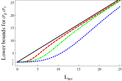
Figure 1: (Color online) The dependence on Linv\mathrm{L}_{\textrm{inv}} of the new bound (6) for some fixed values of ℛinv\mathcal{R}_{\textrm{inv}}: ℛinv=103\mathcal{R}_{\textrm{inv}}=10^{3} - red/dashed, ℛinv=104\mathcal{R}_{\textrm{inv}}=10^{4} - green/dashed-dotted, ℛinv=105\mathcal{R}_{\textrm{inv}}=10^{5} - blue/dotted. The black line represents the reference bound (2). All bounds are above the Heisenberg bound 3/23/2.

IV Discussion

In this Section I would like to present the connection of the new uncertainty relation (6) with the previous results (1) and (2). First of all we shall note, looking at the expression (36), that

Ω⁡(0,ℛ)=32, and limℛ→∞Ω⁡(L,ℛ)=32.\Omega\left(0,\mathcal{R}\right)=\frac{3}{2},\>\textrm{ and }\quad\lim_{\mathcal{R}\rightarrow\infty}\Omega\left(\mathrm{L},\mathcal{R}\right)=\frac{3}{2}. (41)

These results mean that in both cases, when the angular momentum is L=0\mathrm{L}=0 or when the variance ℛ\mathcal{R} is very large, we have no improvement of the ordinary Heisenberg uncertainty relation (1). This conclusion is in a full agreement with logical expectations. Furthermore, it is easy to check that

Ω⁡(l⁡(l+1),0)=32+l,\Omega\left(\sqrt{l\left(l+1\right)},0\right)=\frac{3}{2}+l, (42)

what coincides with the uncertainty relation (2). The value ℛ=0\mathcal{R}=0 means that the state is a true eigenstate of L^2\hat{L}^{2} (or L^inv2\hat{L}_{\textrm{inv}}^{2} in a general reference frame) and the average value L2\mathrm{L}^{2} must be equal to l⁡(l+1)l\left(l+1\right) where ll is related quantum number. Fig. 1 summarizes these observations.

V Conclusions

I this paper I have discussed the Heisenberg uncertainty relation for position and momentum with additional information about angular momentum. I derived new lower bound for the product of standard deviations σr​σp\sigma_{r}\sigma_{p} which depends on the average value and the variance of the L^inv2\hat{L}_{\textrm{inv}}^{2} operator. This operator is a square of the angular momentum operator defined in the reference frame where ⟨𝒓⟩=0=⟨𝒑⟩\left\langle\boldsymbol{r}\right\rangle=0=\left\langle\boldsymbol{p}\right\rangle. I showed that the relation (6) links the ordinary Heisenberg uncertainty relation (1) with stronger relation (2) valid for the eigenstates of L^inv2\hat{L}^{2}_{\textrm{inv}}.

Acknowledgements.
I am especially grateful to Iwo Białynicki-Birula for long discussions and several important comments. Furthermore, I would like to thank all members of the Atomic Physics Group from University of Granada for their kind hospitality and fruitful discussions. Finally, the referee deserves thanks for his/her accurate remarks, that help me clarify the main message of this paper. Financial support by the Grant of the Polish Ministry of Science and Higher Education for years 2010-2012 is gratefully acknowledged.

References

  • [1] W. Heisenberg, Z. Phys. 43, 172 (1927).
  • [2] E. Kennard, Z. Phys. 44, 326 (1927).
  • [3] P. Sánchez-Moreno, R. González-Férez and J. S. Dehesa, New J. Phys. 8, 330 (2006).
  • [4] C. Bracher, Am. J. Phys. 79, 313 (2011).
  • [5] M. E. Grypeos, et al., J. Phys. A 37, 7895 (2004).
  • [6] I. Bialynicki-Birula and J.Mycielski, Commun. Math. Phys. 44, 129 (1975).
  • [7] I. Bialynicki-Birula, Phys. Rev. A 74, 052101 (2006).
  • [8] S. Zozor, M. Portesi, P. Sánchez-Moreno, and J. S. Dehesa, Phys. Rev. A 83, 052107 (2011).
  • [9] J. C. Angulo, Phys. Rev. A 83, 062102 (2011).
  • [10] P. Sánchez-Moreno, A. R. Plastino, and J. S. Dehesa, J. Phys. A 44, 065301 (2011).
  • [11] P. Sánchez-Moreno, S. Zozor, and J. S. Dehesa, J. Math. Phys. 52, 022105 (2011).
  • [12] E. Romera, P. Sánchez-Moreno, and J. S. Dehesa, J. Math. Phys. 47, 103504 (2006).
  • [13] Á. Guerrero, P. Sánchez-Moreno and J. S. Dehesa, Phys. Rev. A 84, 042105 (2011).
  • [14] I. A. Howard, N. H. March, and L. M. Nieto, Phys. Rev. A 66, 054501 (2002).
  • [15] J. S. Dehesa, R. González-Férez, P. Sánchez-Moreno, and R. J. Yáñez, New J. Phys 9, 131 (2007).
  • [16] I. Bialynicki-Birula, Z. Bialynicka-Birula, arXiv:1110.2415v1 (2011) .
  • [17] I. Bialynicki-Birula, M. Cieplak, J. Kamiński, Theory of Quanta, Oxford University Press (1992).