Maximally entangled gapped ground state of lattice fermions

The fermionic model employed in this work is inspired by experiments with ultracold atomic gases. Numerous groups have confined both bosonic and fermionic atoms in periodic potentials formed from interfering lasers, known as optical lattices [27, 28]. These lattices can confine different spin components of the same bosonic species in independent, overlapping optical lattices [29, 30]. The structure of these lattices is highly flexible [31], and periodic double-well potentials for bosons have been been the subject of particularly intense investigations [32, 33, 34, 35, 36]. In another recent development, an ultracold gas consisting of a mixture of three different spin components of the fermionic atom ⁶Li has been realized in an optical trap [37, 38]. Ultracold fermionic gases of both ⁴⁰K and ⁶Li have been loaded into periodic optical lattices with highly controllable geometries and trapping parameters [39, 40, 41, 42]. It is reasonable to assume that these various techniques could be combined in the future, with multicomponent fermions in three overlapping double-well optical lattices, each confining a different spin component.

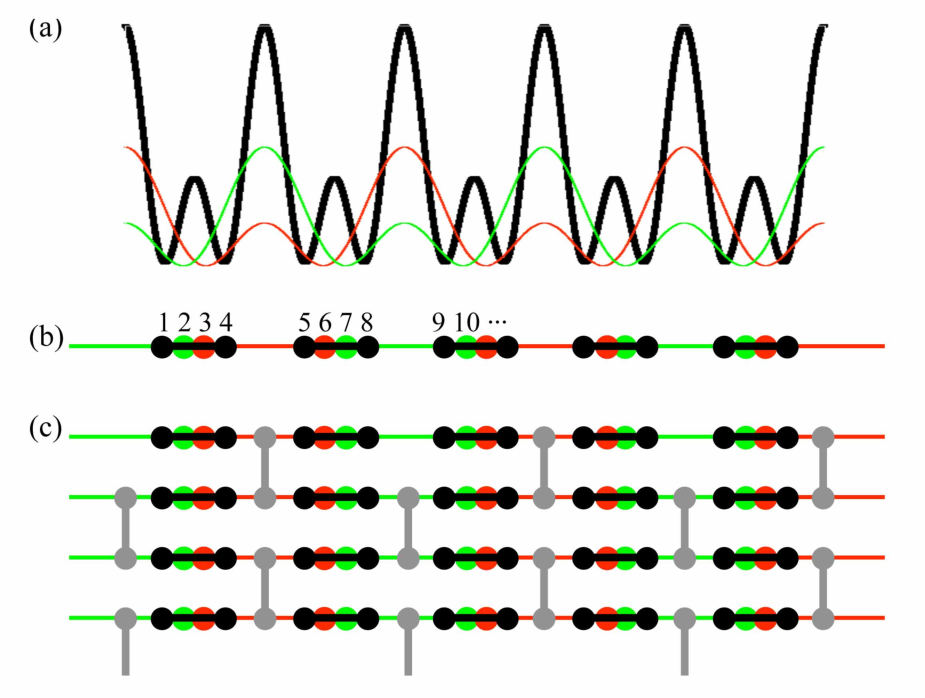
Consider the potentials depicted in Fig. 1(a), corresponding to three overlapping one-dimensional two-site lattices. It is assumed that each sublattice can confine only one particular spin projection of a fermion with pseudospin $s=1$ (corresponding to real spin $s\geq 3/2$ with all but three spin projections frozen out); the spin projections will be labeled $\uparrow$, $o$, and $\downarrow$. The potential shown as a black curve is assumed to confine only the spin $o$, and could be obtained using two potentials with amplitudes $V_{1,o}$ and $V_{2,o}$ and with one wavelength $\lambda$ half as large as another:

Likewise, the potentials seen by the $\uparrow$ and $\downarrow$ spin projections (green and red curves in Fig. 1(a), respectively) would be generated by wavelengths that were twice as long as for projection $o$, and offset relative to each other:

The relative height of the barriers is then set by the ratio $V_{1,\sigma}/V_{2,\sigma}$. Within the tight-binding approximation, assuming the atoms can only tunnel through the lower barrier of a given sublattice, the Hamiltonian becomes

where $f^{{\dagger}}_{i,\sigma}$ ($f_{i,\sigma}$) creates (annihilates) a fermion with spin projection $\sigma$ at site $i$. The $\tau_{\sigma}$ correspond to hopping amplitudes, the exact values of which are unimportant for the present work.

There is no tunneling permitted between different sublattices, but nevertheless fermions with different spin projections must anticommute if the sublattices overlap: if a fermion with one spin projection tunnels past a fermion with another spin projection, the total wavefunction picks up a negative sign. This is because it is impossible to distinguish if the fermions interchanged their spin labels (switching places) during the transit, or remained the same. At the same time, it is unnecessary to impose antisymmetrization on fermions that can never overlap in practice. For example, a $o$-projection fermion in site 1 in Fig. 1(b) needs to be antisymmetrized only with fermions in sites 2, 3, and 4; the tunneling barrier between sites 4 and 5 is assumed to be so large as to prevent any tunneling for $o$-spin projection atoms.

The relative strengths of the tunneling amplitudes are not important for the ground state, as long as they are all non-zero. One may assume that the system is given sufficiently long to equilibrate compared to the tunneling rates. Thus one may choose $\tau_{o}=\tau_{\uparrow}=\tau_{\downarrow}\equiv\tau$ without loss of generality. The Hamiltonian (3) can be further simplified by noting that fermions with a given spin projection are constrained to their respective sublattices. The spin-projection index can therefore be suppressed, corresponding to spinless (fully polarized) fermions. One then obtains the equivalent ‘leapfrog’ Hamiltonian

which is the central model of the current work, and is depicted graphically in Fig. 1(b). Though the Hamiltonian appears to involve third-nearest neighbor hopping, it is in fact obtained by nearest-neighbor hopping on an array of three overlapping two-site sublattices.

Consider only the case where each spinless sublattice is exactly half-filled: each connected double-well indexed by $j$ contains exactly one fermion, $n_{2j+1}+n_{2j+4}\equiv 1$. Mathematically, this could be accomplished by applying a suitable projector to the Hamiltonian (4). In an experiment with ultracold atoms, such a configuration could be obtained by detecting and selectively moving or removing single atoms [43, 44, 45, 46, 47].

Making use of the Jordan-Wigner transformation

the Hamiltonian (4) may be expressed in the spin representation:

which is four-local in marked contrast to that in the fermion representation. Because of the half-filling restriction, the ground state only involves states with Hamming weight $N$ and therefore only involves combinations of the encoded registers

where the state $|{\mathcal{O}}\rangle$ represents the particle vacuum. In other words, the $|\underline{0}_{j}\rangle$ register has the single fermion on the first site of a given double-well indexed by $j$, while the $|\underline{1}_{j}\rangle$ register corresponds to the fermion in the second site.

One can introduce an encoded basis where the operators become $\left(X_{2j+1}X_{2j+4}+Y_{2j+1}Y_{2j+4}\right)/2\equiv\underline{X}_{j}$, $I_{2j+1}Z_{2j+4}\equiv\underline{Z}_{j}$, and $Z_{2j+1}I_{2j+4}\equiv-\underline{Z}_{j}$ (recall the half-filling condition), i.e. $\underline{X}_{j}|\underline{0}_{j}\rangle=|\underline{1}_{j}\rangle$ and vice versa, $\underline{Z}_{j}|\underline{0}_{j}\rangle=|\underline{0}_{j}\rangle$, and $\underline{Z}_{j}|\underline{1}_{j}\rangle=-|\underline{1}_{j}\rangle$. Using $Z_{2j+2}=I_{2(j-1)+1}Z_{2(j-1)+4}=\underline{Z}_{j-1}$ and $Z_{2j+3}=Z_{2(j+1)+1}I_{2(j+1)+4}=-\underline{Z}_{j+1}$, the Hamiltonian (6) in the encoded basis becomes

with $\underline{Z}_{0}=\underline{I}_{1}$. Applying the unitary transformation $\underline{Z}_{j}$ for all $j\in\{1,N-1\}$ performs the maps $\underline{X}_{j}\to-\underline{X}_{j}$, transforming (7) into exactly the same Hamiltonian as the one-dimensional cluster-state Hamiltonian on $N$ qubits, Eq. (1). The ground state of Hamiltonian (7) is therefore immediately obtained by comparing with the usual cluster state, Eq. (2):

where $|\mbox{\boldmath$+$}\rangle\equiv\left(|\underline{0}\rangle+|\underline{1}\rangle\right)/\sqrt{2}$, and the encoded entangling gate is defined as $\underline{CZ}_{j,j+1}\equiv\mbox{diag}\left(1,1,1,-1\right)$ in the space spanned by the vectors $|\underline{0}_{j}\underline{0}_{j+1}\rangle$, $|\underline{0}_{j}\underline{1}_{j+1}\rangle$, $|\underline{1}_{j}\underline{0}_{j+1}\rangle$, and $|\underline{1}_{j}\underline{1}_{j+1}\rangle$. It is clear that the ground state is equivalent to the one-dimensional cluster state, where each qubit is maximally entangled to its neighbor. This entanglement is a direct consequence of fermionic antisymmetry and indistinguishability. The excitations correspond to $\underline{Z}_{i}$ operations on the ground state, which cost energy $\tau$. The energy gap is therefore $\tau$, independent of system size.

Consider the consequences of measuring the position of one of the two fermions in a two-qubit fermionic cluster state. Suppose that the entire system consisted of sites 1, 3, 4, and 6 in Fig. 1(b). In the absence of inert fermions in the unpaired sites 2 and 5, these sites can be ignored, and the ground state of the Hamiltonian (4) is maximally entangled:

In the Fermi-occupation notation, the ground state appears to be separable; however, this ignores the fact that fermions on sites 3 and 4 must anticommute if there is any chance that these fermions can interchange. Consequently, defining the fermionic occupation states in the natural ordering by increasing label $|0110\rangle_{1,3,4,6}=f_{3}^{{\dagger}}f_{4}^{{\dagger}}|{\mathcal{O}}\rangle_{1,3,4,6}$, a negative sign appears on the second line above. If the fermions on site-pairs $\{1,4\}$ and $\{3,6\}$ could never overlap (i.e. there was an impenetrable barrier between them), then the state would be truly separable and no explicit antisymmetrization would be required.

Measurement of the first qubit in encoded state $|\underline{0}_{1}\rangle$ corresponds to the application of the projector $\left({\mathcal{M}}_{1}\right)_{1}=|1_{1}0_{4}\rangle\langle 1_{1}0_{4}|=f_{1}^{{\dagger}}|{\mathcal{O}}\rangle\langle{\mathcal{O}}|f_{1}$, yielding

Likewise, applying the other projector $\left({\mathcal{M}}_{2}\right)_{1}=|0_{1}1_{4}\rangle\langle 0_{1}1_{4}|=f_{4}^{{\dagger}}|{\mathcal{O}}\rangle\langle{\mathcal{O}}|f_{4}$ yields the state

The dependence of the second encoded qubit’s output state on the outcome of the first encoded qubit’s measurement is a direct consequence of the entanglement of the original fermionic state.

It is important to note, and easy to verify, that this result doesn’t depend on how one labels the sites. If the two double-sites were instead labeled $\{1,3\}$ and $\{4,6\}$, so that no negative sign appeared in the ground state (8), the same states would still be obtained after measurement. This is because the result of the measurement operation on the double-site $\{1,3\}$ explicitly depends on the possible existence of a fermion at the intervening site 4. If instead the two double-wells were disconnected (non-overlapping), then there would be no intervening site with which to anticommute, and therefore no dependence of the output on the measurement outcome. In short, the entanglement arises from the fundamental requirement that fermions on the sites 3 and 4 must anticommute when there is the potential for these wavefunctions to overlap.

In order to perform universal gate teleportation using the encoded cluster state, Eq. (10) in the manuscript, it is important to derive expressions for the encoded $\underline{X}$, $\underline{Y}$, and $\underline{Z}$-rotations, Hadamard operator $\underline{H}$, and measurement operators that one would need to apply in order to teleport gates with fermions. The encoded $\underline{Z}$-rotation is straightforward:

where $1-2n_{2j+4}=\underline{Z}_{j}$ is the encoded Z operator. Because $n_{2j+4}=1-n_{2j+1}$ an equivalent expression would be

Thus, $\underline{R}_{Z}(\theta)=e^{-i\theta/2}$ if the fermion is in the first site and $\underline{R}_{Z}(\theta)=e^{i\theta/2}$ if it is in the second, as expected from the qubit encoding. To obtain the encoded $\underline{X}$-rotation, one can make use of the relations

and $\underline{X}_{j}^{2}=n_{2j+1}\left(1-n_{2j+4}\right)+n_{2j+4}\left(1-n_{2j+1}\right)=n_{2j+1}+n_{2j+4}=1$ when each two-site lattice has exactly one fermion. One then finds

One can write $\underline{Y}_{j}=-i\underline{Z}_{j}\underline{X}_{j}=iZ_{2j+1}\underline{X}_{j}$, so that the encoded $\underline{Y}$-rotation is

Finally, the encoded Hadamard gate is $\underline{H}_{j}=\underline{Z}_{j}\underline{R}_{Y}(-\pi/2)_{j}=-\left(1-2n_{2j+1}\right)\underline{R}_{Y}(-\pi/2)_{j}$:

Note that in marked contrast with the qubit representation, in the fermion representation the $\underline{X}_{j}$, $\underline{Y}_{j}$, and $\underline{H}_{j}$ operators acting on encoded qubit $j$ (involving the two sites labeled by $2j+1$ and $2j+4$) are intrinsically non-local, since they depend explicitly on the fermion density at the intervening sites $2j+2$ and $2j+3$. Nevertheless they are fully separable (i.e. not entangling), as will be shown explicitly in the example below. One might ask why they are nevertheless non-local. Suppose that the $\left(1-2n_{2j+2}\right)\left(1-2n_{2j+3}\right)$ term were dropped in expression (9) for the encoded $\underline{X}_{j}$ operator. The operation would then naïvely correspond to an unencoded $X_{j}$ operation, but only in the absence of fermions between sites $2j+1$ and $2j+4$. If there were in fact one fermion occupying either of the intervening sites $2j+2$ or $2j+3$, then hopping between $2j+1$ and $2j+4$ would introduce undesired negative signs to certain matrix elements. Of course, these are exactly the factors that yield the ground-state entanglement in the first place! But they are unwanted in the implementation of $X$, $Y$, and $H$ operations, and so need to be cancelled in the encoded versions $\underline{X}$, $\underline{Y}$, and $\underline{H}$ if necessary. Consider two encoded qubits, for example. The basis is spanned by the vectors $|1100\rangle=f_{1}^{{\dagger}}f_{3}^{{\dagger}}|{\mathcal{O}}_{4}\rangle$, $|1001\rangle=f_{1}^{{\dagger}}f_{6}^{{\dagger}}|{\mathcal{O}}_{4}\rangle$, $|0110\rangle=f_{3}^{{\dagger}}f_{4}^{{\dagger}}|{\mathcal{O}}_{4}\rangle$, and $|0011\rangle=f_{4}^{{\dagger}}f_{6}^{{\dagger}}|{\mathcal{O}}_{4}\rangle$, the encoded Hadamard gate (10) acting on the first encoded qubit is

which is manifestly separable in matrix form even though it appears not to be in the fermion representation (10).

The measurements are made in the local fermion basis, so that

and

In other words, the qubit projectors correspond simply to observing the site indexed by $2j+1$ or $2j+4$ to determine if a fermion is present; if so, it is projected into the encoded state $|\underline{0}\rangle$ or $|\underline{1}\rangle$, respectively.

It is instructive to consider how one would implement one gate teleportation on a two-qubit fermionic cluster state. Suppose that the entire system consisted of sites 1, 3, 4, and 6 in Fig. 1(b) as in the two-qubit example in the previous section, with ground state given by Eq. (8). Suppose that all sources of energy exchange between the system and the environment are eliminated, other than those associated with applied rotations and measurements, so that $|\psi\rangle\equiv|{\rm g.s.}\rangle$. In order to teleport an arbitrary single-qubit gate in a ordinary 1D cluster state, one needs to perform a series of measurements in the $HR_{Z}(\theta)$ basis. The first qubit is to be rotated first by the encoded gate $\underline{R}_{Z}(\theta)_{1}$, then by $\underline{H}_{1}$, and then measured in the computational basis spanned by the states $|\underline{0}\rangle=f_{1}^{{\dagger}}|{\mathcal{O}}\rangle_{1,4}$ and $|\underline{1}\rangle=f_{4}^{{\dagger}}|{\mathcal{O}}\rangle_{1,4}$. Evidently the applied rotations on the first qubit will push $|\psi\rangle$ away from the ground state, though the fermions in all the other double wells remain in eigenstates of the original Hamiltonian. As a consequence, the state of the first qubit will oscillate at a frequency $\tau_{14}/\hbar$. All states and operations can therefore be considered only at $2\pi/\tau_{14}$ intervals. This assumption is not essential, however, as discussed below in Sec. IV.4.

A $\underline{Z}_{1}$-rotation on the first encoded qubit yields

ignoring an overall phase $e^{-i\theta/2}$; subsequent application of an encoded Hadamard operation gives

Measurement of the first qubit in encoded state $|\underline{0}_{1}\rangle$ corresponds to the application of the projector $\left({\mathcal{M}}_{1}\right)_{1}=|1_{1}0_{4}\rangle\langle 1_{1}0_{4}|=f_{1}^{{\dagger}}|{\mathcal{O}}\rangle\langle{\mathcal{O}}|f_{1}$:

Likewise, applying the other projector $\left({\mathcal{M}}_{2}\right)_{1}=|0_{1}1_{4}\rangle\langle 0_{1}1_{4}|=f_{4}^{{\dagger}}|{\mathcal{O}}\rangle\langle{\mathcal{O}}|f_{4}$ yields the state

Thus, the gate teleportation using fermions proceeds exactly as in the usual spin-qubit case, though with an additional overall $\underline{Z}$ operator reflecting the original ground state (8).

Though the Jordan-Wigner transformation is not uniquely defined in two dimensions, the structure of the qubit encoding carries naturally over to dimensions higher than one. A two-dimensional version of the leapfrog Hamiltonian is shown in Fig. 1(c). Two interpenetrating two-site lattices (shown in grey) that are staggered relative to each other are superimposed on an array of one-dimensional leapfrog chains, similar to those discussed above. Each double-well of the new lattices serves to connect adjacent one-dimensional chains, so the sites are situated between a given connected pair in the chains. Again, only a single fermion is allowed to occupy any given pair of sites of the new lattices. The labelling of the sites can be chosen in any convenient way. When writing out the full ground state in terms of the fermion field operators, one need only keep in mind which sites interleave others.

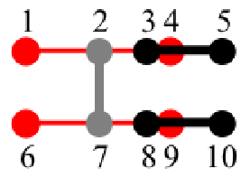
In order to demonstrate that the ground state of the fermionic leapfrog Hamiltonian is computationally universal, it remains to be shown that the presence of the vertical links has the effect of entangling the two horizontal chains. Consider for this purpose a two-dimensional subgraph of the full lattice configuration shown in Fig. 1(c), in which two encoded two-qubit cluster states are coupled together by a single vertical link as shown in Fig. 2. The sites on the top row are labeled 1 through 5 with site 2 the upper partner of the vertical double well, and the bottom three sites are labeled 5 through 10 with site 7 the lower partner of site 2. The Hamiltonian corresponding to this subgraph is

It is simple to verify that the ground state is

If the vertical link (sites 2 and 7) truly entangles the two horizontal chains, then measuring the fermions in all the double wells labeled by $\{1,4\}$, $\{6,9\}$, and $\{2,7\}$ should yield entanglement between the two encoded qubits associated with the double wells labeled by $\{3,5\}$ and $\{8,10\}$, even though there is no explicit link remaining between them. The $\{1,4\}$ and $\{6,9\}$ sites are measured in the encoded $X$ basis, corresponding to the application of an encoded Hadamard gate followed by a computational-basis measurement. The $\{2,7\}$ sites are measured in the encoded $Y$ basis, i.e. the $\{2,7\}$ sites are first transformed by $\sqrt{\underline{X}}$ and then measured in the computational basis. The result doesn’t depend on the order in which these operations and measurements are made, because only Pauli byproduct operators are teleported. Ignoring overall phases the output is

where $m_{i}=\{0,1\}$ are the measurement outcomes and

are local encoded Pauli byproduct operators corresponding to the eight possible outcomes. Thus, the result of these measurements is to maximally entangle the two qubits $|\mbox{\boldmath$+$}\rangle_{3,5}$ and $|\mbox{\boldmath$+$}\rangle_{8,10}$. If the two qubits encoded on sites $\{1,4\}$ and $\{6,9\}$ were originally in the states $|\underline{\psi}_{1}\rangle$ and $|\underline{\psi}_{2}\rangle$, then the result would be the same as that above except with $|\mbox{\boldmath$++$}\rangle_{3,5,8,10}\to|\underline{\psi}_{1}\underline{\psi}_{2}\rangle_{3,5,8,10}$.

The two-qubit example demonstrates how one-dimensional fermionic cluster states can be used in order to perform universal gate teleportation. Nevertheless, it is not apparent how the various encoded operations — the $\underline{R}_{Z}(\theta)$, $\underline{H}$, $\underline{R}_{X}(\pi/2)=\sqrt{\underline{X}}$, and measurements — would be implemented in practice. Of particular concern is that the encoded Hadamard gate and the $\underline{X}$ and $\underline{Y}$ rotations are explicitly non-local in the fermion representation, as shown above [cf. Eqs.(9) and (10)]: all require local hopping on a given pair of sites in a sublattice with an amplitude dependent on the occupancy of intervening qubits on different sublattices. As shown below, it is possible to implement all encoded operations but only if one allows the fermions to explicitly interact.

Consider again the two-qubit example discussed above. All local gates on the first qubit can be performed by the application of the additional two-site hopping Hamiltonians

and

for particular choices of parameters and times. The Hamiltonian (12) is the same as Eq. (4), with the addition of potential energies $V_{1}$ and $V_{4}$ on the two sites of the first double-well. The spin indices $\sigma$ and $\sigma^{\prime}$ in Hamiltonian (13) represent the fermionic spin projection for encoded qubits 1 and 2, respectively. Thus, the fermion encoding qubit 1 is allowed to tunnel between sites 4 and 3 and possibly interact with the inert fermion on site 3.

A fermion may or may not be present on site 3 (if not, then it occupies site 6), so the Hamiltonians (12) and (13) act on two independent two-dimensional blocks. For $H_{a}$, the states in the first block are $\left\{f_{1}^{{\dagger}}f_{3}^{{\dagger}}|{\mathcal{O}}\rangle\,,f_{3}^{{\dagger}}f_{4}^{{\dagger}}|{\mathcal{O}}\rangle\right\}$, while those in the second block are $\left\{f_{1}^{{\dagger}}|{\mathcal{O}}\rangle\,,f_{4}^{{\dagger}}|{\mathcal{O}}\rangle\right\}$. In the first block, a fermion hopping between sites 1 and 4 must cross the fermion in site 3, acquiring a negative sign in the process; the sign change is absent in the second block. But all single-qubit operations on the first qubit must be truly local: the resulting gate $\exp(-itH)$ cannot depend on the state of the second qubit, i.e. the possible presence of a fermion on site 3. For $H_{b}$, the two states in the first block correspond to $\left\{f_{3,\sigma^{\prime}}^{{\dagger}}f_{3,\sigma}^{{\dagger}}|{\mathcal{O}}\rangle\,,f_{3,\sigma^{\prime}}^{{\dagger}}f_{4,\sigma}^{{\dagger}}|{\mathcal{O}}\rangle\right\}$, while those in the second block are $\left\{f_{3,\sigma}^{{\dagger}}|{\mathcal{O}}\rangle\,,f_{4,\sigma}^{{\dagger}}|{\mathcal{O}}\rangle\right\}$. No fermions cross in either block, but additional phases can result from the interaction in site 3 of a fermion with spin $\sigma$ and one with spin $\sigma^{\prime}$.

The most straightforward gate is an arbitrary $Z$-axis rotation on the first qubit, which corresponds to turning on $H_{a}$ for a given time: $\underline{R}_{Z}(-V_{4}t)_{1}=\exp\left[-itH_{a}\left(0,0,V_{4}\right)\right]$ for either block, ignoring an overall unimportant phase. In practise, a strong repulsive potential would be applied to the barrier between sites 1 and 4 to turn off tunneling, and another potential applied to site 4. Next consider the implementation of the encoded Hadamard gate $\underline{H}_{1}$. Applying $H_{a}\left(\tau_{14},-1+\sqrt{2},1+\sqrt{2}\right)$ for a time $t=\pi/\sqrt{8}\tau_{14}$ yields $\underline{H}_{1}$ in the first block and $\underline{Z}_{1}\underline{H}_{1}\underline{Z}_{1}$ in the second. This gate is equivalent to $\underline{CZ}_{12}\underline{H}_{1}\underline{CZ}_{12}$ which is not the desired Hadamard gate. Likewise, the application of $H_{a}\left(\tau_{14},0,0\right)$ for a time $t=\pi/4\tau_{14}$ yields $\underline{CZ}_{12}\underline{R}_{X}(\pi/2)_{1}\underline{CZ}_{12}$ rather than $\underline{R}_{X}(\pi/2)_{1}$. In order to obtain the desired gates, one can apply $H_{b}$ both before and after the $H_{a}$ above. Choosing $H_{b}\left(\tau_{34},\frac{4}{\sqrt{3}},-\frac{1}{\sqrt{3}},\frac{1}{\sqrt{3}}\right)$ for a time $t=\sqrt{3}\pi/2\tau_{34}$ yields $\underline{I}_{1}$ in the first block and $\underline{Z}_{1}$ in the second, i.e. the gate $\underline{CZ}_{12}$. All parameters in $H_{a}$ are assumed to be zero during the operation of $H_{b}$. Because $H_{b}$ also applies a possible phase to the first register of the second qubit, a repulsive $\sigma^{\prime}$ potential should be applied between sites 4 and 6 during its application and removed thereafter. The majority of the state thereby remains in the ground state of the primary governing Hamiltonian.

It is interesting to note that any attempt to perform a local operation $\underline{U}_{1}$ within the inital non-interacting fermionic model instead yields $\underline{CZ}_{12}\underline{U}_{1}\underline{CZ}_{12}$, which is a two-qubit matchgate modulo local operations. For example, attempting $\underline{U}_{1}=\underline{H}_{1}$ produces a maximally entangling gate that is locally unitary-equivalent to the matchgate ${\rm G}_{\rm HH}$ [26]. In order to obtain a true local operation, required for universal MBQC when restricted to computational basis measurements, one must include some kind of fermion-fermion interaction. In the approach above, an additional hopping Hamiltonian with an on-site interaction yields an explicit $\underline{CZ}_{12}$ which can cancel the effective $\underline{CZ}_{12}$ arising solely from fermionic statistics. Because one can construct the SWAP gate from combinations of Hadamards and $CZ$ gates, this approach is the measurement-based analogue of the fermionic circuit model found previously [22].