Probing strongly interacting W’s at the ILC with polarized beams
Abstract
We study the possibility of fingerprinting a strongly interacting boson sector which is consistent with present day LHC searches at the ILC with longitudinal as well as transversely polarized electron and positron beams. We account for the final state interaction using a suitable Omnès formalism in terms of a plausible resonance description, and carry out thorough analyses of cross sections, asymmetries and angular distributions of the . We carry out a comparison with other extensions of the Standard Model, where heavy additional bosons arise naturally. We also consider the effect of the strong final state interaction on a correlation that depends on , where the are the azimuthal angles of decay leptons, and find that it is a useful discriminant.
1 Introduction
A strongly interacting bosons sector is now a definite possibility especially in the light of the present LHC results [1, 2]. If there is no light Higgs, it could be either that it is very massive and could even violate the unitarity bound of TeV, in which case there would be new physics to restore unitarity via strong gauge boson interaction in gauge boson scattering processes, or that there is no Higgs, which is possible if electroweak symmetry were to be broken dynamically through a Landau-Ginzburg type scenario due to the existence of an order parameter , leading again to strong final state interactions(SFI) of the weak gauge bosons. In slight variation to the strong gauge boson interactions without a Higgs boson, the possibility of a light Higgs boson along with a strongly interacting gauge sector has emerged in the recent past. In this scenario, there exists a light Higgs boson, whose dynamics are not strong enough to unitarize the gauge boson scattering. Unlike the case of the SM, the cross section still grows even after crossing the light Higgs resonance.
In most of the phenomenological studies of scenarios without a light Higgs boson, the onset of strong interactions among the gauge bosons is viewed in a fashion very similar to that of the strong interaction dynamics of pions. While pions are considered as the pseudo Goldstone Bosons of chiral symmetry breaking in low energy QCD, the longitudinal modes of the weak gauge bosons are essentially the Goldstone modes of electroweak symmetry breaking (EWSB). This analogy, along with the equivalence theorem of weak gauge bosons, which states that at high energies (compared to their masses) the gauge boson scattering cross sections are essentially equal to the cross sections of the Goldstone Boson scattering [3]. It is possible to have some understanding of the gauge boson scattering in this strongly interacting regime: at the electroweak scale, a “chiral effective Lagrangian” [4] can be constructed along the lines of low-energy QCD, with different interaction terms among the gauge bosons with appropriate coefficients. These coefficients can in principle be computed using the underlying theory at high energies. Unlike in the case of pion interactions, where the underlying theory is QCD, such a theory is not known in the weak interaction case. In the absence of such a theory, these coefficients are considered as parameters to be fixed from experiments. One important feature of strong pion interactions is the existence of various resonances in their scattering. Therefore, adapting a similar scheme for the weak gauge boson scattering implies the existence of resonances beyond the unitarity violating scale. In the chiral effective Lagrangian approach, effect of such resonances at electroweak scale can be accommodated into the various coefficients of the Lagrangian by integrating out the heavy resonances. Early phenomenological studies of strong gauge boson, in the absence of a light Higgs, relevant to LHC are summarized in Ref. [5, 6]. Gauge boson scatterings in processes like , where were computed within, what is known as, the equivalent gauge boson approximation (EGBA) [7]. In such an approximation the scattering cross section is folded with the probability distribution of and bosons contained in the proton. More recently various analyses have pointed out the inadequacy of the EGBA, suggesting that a full analysis of the process is necessary [8, 9] to take into account the non-negligible contributions coming from off-shell gauge bosons, as well as the possibility of the same final state arising through intermediate states other than those with radiation from protons. In particular in Ref. [9] contributions of various different possible resonances in the scattering within the chiral Lagrangian framework, have been included using the event generator called WHIZARD [10] to study the phenomenology at LHC.
Returning now to a light Higgs 115 130 GeV, two distinct cases relevant in this context are with additional Higgs bosons, which restore unitarity [11], and without any other Higgs bosons in the spectrum, in which case unitarity is restored by new physics [12]. In these cases, gauge bosons become strongly interacting after crossing the light Higgs resonance. Thus, even with the discovery of a light scalar particle in the small window available at the LHC [2], a detailed analysis of the gauge boson interactions, especially probing the signatures of their strong interactions in processes with and/or bosons in the final state is essential to understand the mechanism of EWSB, as emphasised by [13, 14]. Phenomenology of such models at LHC are considered in Ref. [11, 12, 15]. A comprehensive review of various models and approaches to study the strong gauge boson interactions may be found in [16].
In the effective phenomenological approach, the underlying theoretical origin of these resonances is not addressed. The ultraviolet completion of such effective theories are expected to explain the origin of such resonances. In most cases, it is argued [9, 13], that the vector bosons are the dominant resonances. Among the renomarlizable theories explaining the origin of vector resonances , the idea of dynamical EWSB of technicolour models [17] proposing a composite scalar sector with a techni- meson playing the role of the vector resonance mentioned above has been studied in detail in the past decades. While aesthetically very pleasing, in their original form, these models fail to comply with electroweak precision measurements. In a philosophically different approach, the BESS (Breaking Electroweak Symmetry Strongly) models [18] consider the resonance as a gauge boson of a hidden , introducing strong interactions in the weak gauge boson sector. This model, again, is ruled out by precision electroweak measurements, unless the is fermiophobic. With the possibility of low energy gravity scenarios arising through large compactified extra space dimensions, an interesting set of models have emerged in the recent past. These Higgsless models [19] have been proposed with gauge theories in five dimensions. In such models the Kaluza-Klein towers of the gauge bosons act as the moderators of unitarity in gauge boson scattering in four dimensions. In a different perspective, in many versions, these models can be considered as four dimensional deconstructed theories with a chain of SU(2) gauge groups [20]. The BESS model above can be considered as some special case of the deconstructed models. A general discussion of relation between the composite models with and without gauge theory is presented in [21]. The effect of such a vector resonance (in the absence of any other resonance) in scattering was recently analyzed in the context of LHC [13, 22]. In these models as well, when the new gauge bosons couple to the SM fermions, evading precision constraints is difficult, but possible with some modifications [23].
Coming to the leptonic colliders, similar to the case mentioned above in the context of LHC, , where have been investigated for strong scattering. A large volume of phenomenological studies available in this case are summarized in Refs. [24, 25]. This process is sensitive to scalar and tensor resonances, as well as the vector resonances arising in gauge boson scattering. On the other hand, the process , which we consider in the present work, has the advantage that only vector resonances are involved. The fact that the cross section (at ILC energies) for is about three orders of magnitude larger than that of also helps the former. For reviews of phenomenological work on based on “chiral electroweak Lagrangian”, see the work of Barklow [26]. Some early analyses of within the framework of the BESS model studied the contribution of the additional in the -channel [27, 28]. These were extended to include the decay spectrum of the ’s with the leptonic energy and angle distributions acting as polarization analyzers [29]. These effects are almost negligible unless one is very close to the new vector resonance, owing to their highly constrained fermionic couplings. However, even in the absence of fermion couplings, these vector resonances can leave their impact through strong final state interactions (SFI) in the same process. In a model independent way, the effect of a single vector boson resonance such as this in the SFI can easily be parametrized by introducing suitable form factors in the partial wave amplitude of . With this philosophy, one may approximate the effect of the resonance through a Gounaris-Sakurai (GS) form factor, as considered in [30], or even through a Breit-Wigner (BW) form factor, as considered in [31]. An improved treatment of vector boson resonance is to introduce a suitable Omnès function. Ref. [32] has used the Omnès function with Padé unitarization method considered to implement the phase shift of the partial wave in . Studies in pair production at a collider is considered in Ref. [33], where again the SFI is modeled through a spin-2 resonance, the effect of which is considered through a BW form factor introduced in the partial wave.
Revisiting the pair production at ILC, in the present work, we study the effect of such a resonance in this process. While inspired by the theoretical scenarios described earlier, we consider a model independent approach in our study. Here, we will follow the treatment adopted in refs. [30, 31, 32], with suitably defined Omnès function to be described. In an earlier analysis of the same process [34], we had considered the effect of the presence of heavy boson, arising in many Grand Unified scenarios including the , Left Right Symmetric Model (LRSM) and the Alternate Left Right Symmetric Model (ALRSM) [35], as well as in the Little Higgs Models (LHM) [36]. With the effect of SFI with vector resonance expected to mimic the presence of a in the -channel, it is prudent to distinguish between these. The role of beam polarization at the ILC in probing new physics and disentangling various possible scenarios have been demonstrated through many examples (for example, see [37] for a recent review). In this work we exploit the potential of beam polarizations, both longitudinal polarizations (LP) and the transverse beam polarization (TP) expected to be available at ILC to study the new physics effects. Note that the possibilities with TP have not received any attention in studies involving SFI, although studies on effects of anomalous couplings in case of pair production at linear colliders are considered by Refs. [38, 39, 40].
The plan of this article is the following. In Section 2 we very briefly review the formalism to introduce the SFI through a modification of the partial wave with the Omnès function as applied to the process under consideration. In Section 3 we categorise the different type of polarizations considered in our analyses. In Section 4 we discuss different observables sensitive to the new effect, and present our numerical results, where a comparison with the effect of in the same process is considered. In this section we also attempt to discriminate between the two effects with the help of various observables. In Section 5, we probe the effects, through the azimuthal distribution of the decay leptons, and the single energy distribution. In Section 6 we provide discussions and conclusions. In Appendix A we present some details of the parametrizations used in Section 2.
2 Strong Final State Interaction in channel

The process in the SM proceeds through the -channel exchange of and , and a -channel exchange, as shown in Fig. 1.
In this work since we are interested in SFI arising in the EWSB sector, only the amplitudes involving longitudinal ’s (denoted as henceforth) are modified, leaving the helicity amplitudes involving transverse ’s unaffected. The strong interaction through vector resonance affects only the partial wave. Thus, representing the SFI through an Omnès function , the invariant amplitudes involving are modified. Noting that the and exchange -channel contributions are pure waves, whereas the exchange -channel has all partial waves with , the amplitude corresponding to -channel of the production is modified as:
| (1) |
The effect of the SFI in the -channel can be presented in the modification of the partial wave amplitude, leaving the other partial waves unaffected. Schematically therefore
| (2) |
We have to isolate the =1 partial wave, with the helicity amplitude for defined in terms of partial waves as,11 1 Note, that there has been an error in the formalism presented in Ref. [31], which has also unfortunately trickled into the numerical effects. In eq. (12) of Ref. [31] with the choice for projection made therein, a factor of is missing in the second term, on the right hand side. Whereas in Ref. [30] it was apparent that there are no significant effects in the cross section at centre of mass energies far away from the mass region of the resonance, the contrary finding was reported in Ref. [31] which showed a significant deviation from the situation when there are no SFI already at a c.m. energy of 500 GeV. This is traced to the error noted here.
| (3) |
where
| (4) |
is the relevant rotation function. The partial wave is isolated by the projection,
| (5) |
The rest of the amplitude with is obtained by noting,
| (6) |
We can rewrite eq. (2) as:
| (7) |
The Omnès function, describes the effect of the vector resonance arising in the strong interaction of the final state ’s. To describe this function, we consider a simple parametrization of the resonance through its mass, and its width, . We chose the mass to vary from the unitarity limit 1.2 TeV to 2 TeV, as the effect of a resonance with mass beyond a few TeV is expected to be small at an ILC running up to centre of mass (c.m.) energy of 1 TeV. For the choice of width, we rely on the constraints employed by the low energy chiral QCD on . Accordingly we consider the relation
| (8) |
where = 246 GeV is the Higgs vacuum expectation value in the SM. While adopting this choice for most of our analyses, we study the effect of varying , considered as a free parameter, for certain observables in the next Section. For one choice of = 1200 Gev, we vary in the range (50 140) GeV, to study the effects of such flexibility on one of the observables.
Given and the phase of the form factor may be obtained either from a K- matrix, or from GS or BW parametrization as explicitly given in Appendix A. Given we obtain the Omnès function,
| (9) |
Note that the form factor itself for a single channel elastic scattering is related to by [41]
| (10) |
The constants etc. are fixed from additional inputs from the underlying theory, or experiments, which we assume to be large. Since the correct prescription is the use of the Omnès function, for purposes of comparison we study the effect of replacing in some instances in the next section. We treat GS and BW parametrizations as low energy representation of the form factor only to generate . However to contrast these effects we tabulate explicitly the values due to GS and BW parametrizations, and the corresponding Omnès function for the energies of interest given (and ). This is shown in Table 1, where we give the relevant Omnès function corresponding to the form factors used, for typical ILC energies of = 500, 800 and 1000 GeV.
| (GeV) | GS | Omnès function | BW | Omnès function | ||
|---|---|---|---|---|---|---|
| (GeV) | eq. (8) | (GeV) | eq. (22) | from GS | eq. (28) | from BW |
| 500 | 3.849 + 0.055 | 1.223 + 0.017 | 0.993 + 0.083 | 1.198 + 0.099 | ||
| 1200 | 95 | 800 | 5.750 + 0.347 | 1.827 + 0.110 | 0.982 + 0.135 | 1.727 + 0.237 |
| 1000 | 10.225 + 1.803 | 3.248 + 0.573 | 0.939 + 0.240 | 2.979 + 0.760 | ||
| 500 | 4.599 + 0.058 | 1.122 + 0.014 | 0.982 + 0.131 | 1.080 + 0.014 | ||
| 1600 | 224 | 800 | 5.570 + 0.242 | 1.361 + 0.059 | 0.969 + 0.173 | 1.234 + 0.220 |
| 1000 | 6.862 + 0.590 | 1.676 + 0.144 | 0.952 + 0.214 | 1.468 + 0.329 | ||
| 500 | 5.470 + 0.064 | 1.081 + 0.013 | 0.961 + 0.193 | 1.013 + 0.203 | ||
| 2000 | 438 | 800 | 6.169 + 0.234 | 1.219 + 0.046 | 0.942 + 0.233 | 1.041 + 0.258 |
| 1000 | 6.941 + 0.474 | 1.372 + 0.094 | 0.926 + 0.263 | 1.117 + 0.317 |
3 Beam Polarization
The use of beam polarization at ILC will significantly benefit the physics program: it is very useful in searches for new physics with small deviations from SM cross sections in two ways. Firstly, in many cases, suitably chosen beam polarization combinations can enhance the signal, and suppress the background. Secondly, it is possible to construct clever observables incorporating the beam polarization information. At the ILC, a beam polarization (both transverse as well as longitudinal) of 80% for electrons and 30% for positrons at the interaction point is proposed, with a possible upgrading to about 60% for the positron beam. As a recapitalation we will describe how the process under consideration is affected by beam polarization. The production at ILC considered here is sensitive to beam polarization, and in the following we will explain how to exploit this to our advantage. For the purpose of clarity and to set up the stage for our discussions in what will follow, we present the cross sections of at GeV with different beam polarizations and final state polarizations, in Table 2. It can be clearly seen from the table, that the different helicities production cross section depend on initial beam polarizations. Note that the dominant -channel is absent in the case of right-polarized electron beams.
| (pb) | ||||
| -1 | -1 | 0.0003 | 0.0010 | 0.0 |
| -1 | 0 | 0.0191 | 0.0541 | 0.0024 |
| -1 | 1 | 3.4943 | 10.063 | 0.2795 |
| 0 | -1 | 0.0032 | 0.0084 | 0.0011 |
| 0 | 0 | 0.0468 | 0.1124 | 0.0263 |
| 0 | 1 | 0.0191 | 0.0541 | 0.0024 |
| 1 | -1 | 0.0921 | 0.2653 | 0.0074 |
| 1 | 0 | 0.0032 | 0.0085 | 0.0011 |
| 1 | 1 | 0.0003 | 0.0010 | 0.0 |
3.1 Longitudinal Polarization
In the case of longitudinal beam polarization, the dependence of the cross section to the polarization is usually parametrized through the degree of polarization, which is defined as , where denote the number of left-polarized and right-polarized electrons (or positrons) respectively. For an electron beam with degree of longitudinal polarization and a positron beam with degree of polarization , the total cross section in the centre of mass frame with c.m. energy is given by,
| (11) |
where . is the helicity amplitude with right-handed electron and left-handed positron, and is the helicity amplitude with left-handed electron and right-handed positron. The helicity amplitudes we used to compute are those given in Ref. [42] in the SM case, and the effect of SFI is introduced through the Omnès functions described in Section 2.
3.2 Transverse Polarization
At the ILC, with the help of the proposed spin rotator scheme the longitudinal beam polarization can be reoriented to achieve TP of the same degree [37]. As explained below, the transverse polarization directions can be used to define the azimuthal direction of the boson produced. For arbitrary polarization of the initial beams, the expression for the differential cross section in eq. (11) is modified to [43, 40, 38]
| (12) | |||||
where is the azimuthal angle of the , in the reference frame with axis defined along the transverse polarization direction of the electron and the positron (with ). The polarization vectors of the electron and positron beams can then be written as,
| (13) |
respectively. The degrees of polarization satisfy the relation, . For simplicity and clarity of discussion, we consider pure transverse polarization, setting for our analyses with TP.
4 Numerical Analyses with
In this section we present our numerical analysis for the process in the presence of SFI and the other models considered in the Introduction along with the SM without SFI. We first investigate the total cross section, followed by the angular distribution of the , the fraction of the emitted in the backward hemisphere along with the left-right asymmetry. The analyses with TP in the initial state is also considered in this section.
4.1 Total Cross Section
We start our analyses with the first observable, where the total cross section with longitudinal beam polarization is considered, as given in eq. (11).

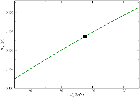
As demonstrated in Section 2 the naive form factor like the GS or BW need to be improved through the description of an Omnès function. While we have demonstrated this by a comparison table in Table 1 we will further consider the effect specific to . Fig. 3 shows the total unpolarized cross section as a function of for , for a given resonance in the case of GS form factor and the relevant Omnès function obtained from it compared with the SM. We heve used GeV and GeV. In the case of the form factor itself, the large deviation present throughout the range of centre of mass energy considered, which is likely to be in conflict with the existing experimental observations (for the parameters considered here), further emphasizes the need for the present approach. Accordingly, we consider the Omnès function for our further analyses. The width, although motivated by the chiral QCD, is put in an ad hoc manner. Sensitivity of our results to the width of the resonance need to be checked. Fig. 3 shows the dependence of the cross section of production at GeV on the width of a resonance at GeV. The cross section changes by about 1% either way from the value obtained using the width obtained from eq. (8), GeV, demonstrating the robustness of the parametrization.


In order to understand the behaviour of the cross section with the use of different form factors as sources for , we present in Fig. 5 the total cross section for beam polarizations22 2 Throughout this article, when we consider longitudinal polarization we assume transverse polarization is absent, and therefore and . of = 0.8 and plotted against the c.m. energy, for three different sets of resonance parameters along with the SM expectation. When the effect of BW resonance is compared with a more complex GS form factor, the difference is not noticeable. Henceforth, we will present our results for the Omnès function obtained using a GS form factor, with judiciously (but arbitrarily) chosen = 1600 GeV and width computed from eq. (8).
Anticipating a symmetric, centrally peaked, distribution of , a cut applied on the production angle can select the most favourable phase space. In Fig. 5 the total cross section of the is presented for same beam polarizations as above, plotted against the c.m. energy with a cut of 0.5, with GS Omnès and Non Resonant models (NR). We have checked that compared to a situation with unpolarized beams, the contrast to the SM case is enhanced, and the sensitivity to effect of SFI is improved considerably, and likely to be observed, achievable at = 500 - 1000 GeV. We present the values of cross section corresponding to the case above, at and GeV in Table 3. For comparison we also present the corresponding values of cross section in the case of selected models discussed in Introduction.
| (pb) | |||||
| Model | 500 GeV | 800 GeV | 1000 GeV | ||
| SM | 0.053 | 0.021 | 0.013 | ||
| Omnès fn | 0.066 | 0.038 | 0.037 | ||
| NR | 0.055 | 0.023 | 0.015 | ||
| 0.8 | -0.6 | ALRSM | 0.044 | 0.011 | 0.002 |
| LRSM | 0.045 | 0.012 | 0.005 | ||
| 0.052 | 0.020 | 0.012 | |||
| LHM | 0.095 | 0.073 | 0.073 | ||
Cross section with transversely polarized ’s ( in the final state are not affected by the SFI, as is clear from our analysis in Section 2. However for the models, this channel is also affected by new physics. While the effect of this in the total cross section is negligibly small, in the following we will describe some observables with in the final state. The inclusion of the initial beam polarization with = -0.8 and = 0.6 enhances the statistics, but the new physics effects are similar to the unpolarized beam case. Henceforth we have therefore considered only = 0.8 and = -0.6 and the case of unpolarized beams.
4.2 Angular Distribution of and
We now consider the angular distribution of the , with both ’s in the final state being longitudinally polarized in Fig. 7 at c.m. energy of 800 GeV, for the different scenarios considered. We have considered = 1600 GeV as our representative point here, and the initial beams are polarized. In the same figure we also plot the effect of generic models considered in Ref. [34], for the parameter values used in accordance with electroweak precision results. In our study for the models, we consider the mixing angle = 0.003 and = 0.12 GeV. For LHM, = 1 TeV and = 0.45 is considered satisfying the electroweak constraints. Clearly, it is hard to distinguish between all and the SFI with the angular distribution. While all the models show similar angular dependence, the and LR models demonstrate a qualitatively different behaviour compared to the SFI and LHM models, in the sense that, while the former models show a diminishing effect, the latter models provide an enhancement in the angular distribution with respect to the SM value. We emphasize that the parameter set used in the case of models were the most optimistic scenarios (with the largest possible deviation consistent with the existing experimental constraints). Therefore, it is possible to expect larger deviations than those allowed by typical models here within the LHM as well as SFI. While this itself could act as a model discriminator, we notice that, the SFI is present only in the case of final state, whereas the models including the LHM can affect the case with in the final state. When both are transversely poalrized in the final state, no effect of SFI or is observed. This is because , are mostly produced through the -exchanged -channel, whereas the affects the -channel only. Thus, with one of the transversely polarized and the other longitudinally polarized, models sensitivity can be observed with no influence from SFI. Note that the models including the LHM affect the process through changed SM couplings, as well as through the presence of a vector boson resonance. But the above statements are nevertheless true numerically, and has been checked explicitly. In Fig: 7 we plot the angular distribution of with in the final state, at the same c.m. energy of GeV and initial polarization as in the earlier case of . Except the LHM, other models show insignificant deviation. Furthermore, the deviations are qualitatively different. Thus, results presented in Fig. 7 and Fig. 7 together will be able to distinguish between SFI, LHM and other models.


4.3 Forward Backward Asymmetry
Establishing a vector resonance, and further discriminating different prospective models through the above angular distribution could be a challenge to the experiments, especially considering the small cross sections involved, and efficiencies of reconstructing final state polarizations. We therefore look next at the integrated observables. Integrating the polar angular distributions, we define the Forward-Backward (FB) asymmetry,
| (14) |
or, equivalently, the fraction of the ’s emitted in the backward hemisphere,
| (15) |
These two observables are related to each other by . Fig. 9 presents of the unpolarized with initial beam polarization of = 0.8 and = -0.6. The behaviour is similar to the case of angular distributions, with a diminishing effect from models other than LHM, while the SFI and LHM showing an enhancement. Reading from Table 4, at GeV, 6% of the events are in the backward region. In the presence of SFI, this is substantially increased to a 9%, while for LHM it is more than doubled to 13%. Other models have smaller effect with LRSM and ALRSM showing about 4-5 %, while remaining at 6%. Recall that we have not considered any angular cut here. As in the case of total cross section discussed above, an angular cut will considerably enhance this effect, with comparatively smaller cost in terms of statistics. Also it may be noted that, the small fractions shown here are a little deceptive. With the cross section at 0.3 pb, for a moderate integrated luminosity of 100 fb-1, 6% of the events amount to about 2000 events. Even after putting in a BR ( for semi-leptonic channel) and reconstruction efficiency (), a few hundred events will remain. Certainly, a measurement of increase by 9% or 13% is conceivable in this case. At GeV, the deviations are smaller. SFI improves the fraction to 10.4% from the SM value of 9.4%, while LHM deviates to a much larger 12.8%. Other models reduces the fraction with ALRSM giving the largest fraction of 8.3%. Again, the cross section is increased by a few times, but, it is perhaps very difficult to see the effect at a per - cent level. It is possible to see the effect of LHM at high luminosity. Without beam polarization, as presented in Table 4, the SFI improves the 2.4% value of SM to a 3%, while all other models show smaller effects. With a total cross section about 3.7 pb, the statistics is improved by an order of magnitude. Even then this will require a somewhat larger luminosity to make any meaningful analysis. At GeV, there is no observable deviation for any models. In the case of GeV, the picture is very similar to that of GeV, with some marginal improvement for all models except ALRSM. In the case of ALRSM, the effect is comparable to that of SFI, but while in the former case it is a diminishing effect, the latter case is an enhancement. The advantage of beam polarization is evident from the above analysis.


In Table 4 we also present the case of . As expected there is no effect of SFI here, as it affects only channel. With unpolarized beams, except the ALRSM, which shows a change of 2% in the fraction at GeV and about 4% at GeV, all models show very small effects. Even these effects of ALRSM are not very promising. Thus, practically, there is no effect from any models, and thus, a comparison of unpolarized with is not very illuminating from the point of model discrimination. The situation is changed for better with the beam polarization considered. Largest deviation is in the LHM taking the SM value of the fraction of about 29.8% to 41% at GeV and to 43.4% at GeV. Even such large deviations may not be visible owing to very small cross section available in this channel. Compared to the unpolarized ’s, the cross section is reduced by a factor of about 50, and we need to also consider the efficiency of polarization measurement. So, overall the number of events at 100 fb-1 may even be smaller than 10. This will certainly need very high luminosity to make any statement. The efficiency to measure polarization of both from an event is small, compared to the case with polarization of only one of it measured. It will be beneficial if one considers the case, where one of the is longitudinally polarized, and the other unpolarized. In , only about 12% of the contribution comes from , as seen from Table. 2, in case of = 0.8 and = 0.6. The behavioural pattern will therefore be the same as , due to which we donot present the results here.
| () | () | ||||||||
|---|---|---|---|---|---|---|---|---|---|
| Model | 500 | 800 | 1000 | 500 | 800 | 1000 | |||
| (GeV) | (GeV) | (GeV) | (GeV) | (GeV) | (GeV) | (GeV) | |||
| SM | 0.037 | 0.024 | 0.021 | 0.110 | 0.099 | 0.097 | |||
| Omnès fn. | 1600 | 0.039 | 0.030 | 0.031 | 0.110 | 0.099 | 0.097 | ||
| NR | 0.037 | 0.025 | 0.022 | 0.110 | 0.099 | 0.097 | |||
| 0 | 0 | ALRSM | 1600 | 0.035 | 0.022 | 0.017 | 0.102 | 0.077 | 0.059 |
| LRSM | 1600 | 0.037 | 0.025 | 0.022 | 0.111 | 0.102 | 0.104 | ||
| 1600 | 0.037 | 0.027 | 0.025 | 0.114 | 0.113 | 0.123 | |||
| LHM | 1550 | 0.036 | 0.024 | 0.021 | 0.108 | 0.104 | 0.117 | ||
| SM | 0.094 | 0.063 | 0.055 | 0.306 | 0.298 | 0.295 | |||
| Omnès fn. | 1600 | 0.104 | 0.092 | 0.108 | 0.306 | 0.298 | 0.295 | ||
| NR | 0.096 | 0.067 | 0.059 | 0.306 | 0.298 | 0.0295 | |||
| 0.8 | -0.6 | ALRSM | 1600 | 0.083 | 0.042 | 0.024 | 0.142 | 0.286 | 0.228 |
| LRSM | 1600 | 0.085 | 0.046 | 0.030 | 0.287 | 0.234 | 0.167 | ||
| 1600 | 0.092 | 0.061 | 0.051 | 0.303 | 0.288 | 0.276 | |||
| LHM | 1550 | 0.128 | 0.132 | 0.155 | 0.361 | 0.410 | 0.434 | ||
4.4 Left Right (LR) Asymmetry
We now turn our attention to an asymmetry constructed with the help of beam polarization. The differential left-right asymmetry is defined as
| (16) |
where is the scattering angle. In Fig. 9, we plot the deviation from the SM case,
| (17) |
as a function of for the different models considered, at = 800 GeV. Clearly, the qualitatively different features are potential model discriminators. In a role reversal compared to the earlier observables, here the models show enhancement in the asymmetry compared to the SM case, while the LHM and the SFI show a diminishing effect. The above analyses was done with idealistic beam polarization. More realistic computations with = 1 can be done in the future.
However it is worth noting, within the SM, at 500 fb-1 lumunosity about 12500 events are expected in the backward hemisphere for and , and about 1000 events in the case of and in the semileptonic channel with a detection efficiency of about 65%. This leads to an asymmetric number of events of about a 11500, and a 5% change in this, as is the case with SFI, is very likely to be measurable. If we can measure the asymmetry at 1-2 % level, it is possible to distinguish between the SFI and LHM through a comparison of asymmetries in the forward and backward hemispheres, or even just by considering only the backward region. The differential asymmetry (eq. 16) integrated over the forward hemisphere at three different c.m.energies are presented in Table 5. The effect of SFI is doubled to about 10% deviation from the SM case at GeV with similar increase in other models, where discrimination of models is even more promising, although the actual number of events will come down.
| () | () | |||||
|---|---|---|---|---|---|---|
| Model | 500 | 800 | 1000 | 500 | 800 | 1000 |
| (GeV) | (GeV) | (GeV) | (GeV) | (GeV) | (GeV) | |
| SM | 0.891 | 0.898 | 0.900 | 0.705 | 0.678 | 0.671 |
| Omnès fn. | 0.877 | 0.853 | 0.819 | 0.697 | 0.669 | 0.662 |
| NR | 0.887 | 0.890 | 0.890 | 0.702 | 0.676 | 0.669 |
| ALRSM | 0.938 | 0.968 | 0.988 | 0.738 | 0.744 | 0.814 |
| LRSM | 0.911 | 0.950 | 0.982 | 0.763 | 0.850 | 0.948 |
| 0.898 | 0.916 | 0.933 | 0.739 | 0.777 | 0.838 | |
| LHM | 0.866 | 0.851 | 0.839 | 0.766 | 0.793 | 0.800 |
4.5 Azimuthal distribution of
We now construct some observables with TP, discussed in Section 3.2. Notice that in eq. (12) are computed by setting , and thus automatically reproduce the null theorem, stating that the cross section with transversely polarized beams averaged over the azimuthal angle is the same as the cross section with unpolarized beams, in agreement with the arguments presented for general collisions with chirality conserving interactions (massless electrons) [43]. We have suppressed the helicity information of final state ’s in the invariant amplitudes defined in eq. (12). The SFI affects the partial wave amplitude of for the longitudinal ’s. TP case differs from the unpolarized and longitudinally polarized beam case through the interference of the two amplitudes, .
In Fig. 11 we present the deviation from SM in azimuthal distribution for different scenarios considered with unpolarized in the final state, where we define :
| (18) |
The NR models are indistinguishable from SM, whereas SFI shows about 2% deviation. In case of the models, LHM has the most significant effect with about 7-10% deviation, but the other models have least significant effect. Note that what is plotted is the deviation from the SM case. Therefore the modulation actually shows a dependance different from that in the SM case. This modulation itself is about 2% in the case of LHM, while the effect is negligible for all other models. When the polarization of is considered, in the presence of TP, the new physics effects are significantly enhanced. Fig. 11 shows the above deviation, eq: (18) for all the scenarios with in the final state. It is the most sensitive channel, to look for effects of new physics. However measurement through this channel depends on the efficiency of the polarization measurement as discussed before, and a very high luminosity. The alternative will be to measure the polarization of one of the and select the events with in the final state. An analyses of this channel will also enhance the new physics effect.


The TP case has an interesting feature of receiving contribution from the imaginary part of the amplitude, which is only present in case of SFI. The size of the contribution from Im in eq. (12), due to SFI can be estimated by considering the following asymmetry:
| (19) |
Fig: 13, shows the contribution from the imaginary part of the amplitude, in case of unpolarized . It can be seen the imaginary part is too small to be measured, unless we have a very high luminosity, and we are very close to the resonance. The contribution from the imaginary part can be measured by other methods, which will be discussed in the next section.


5 Inclusion of Decays
The observables which were considered with unpolarized and longitudinal beams, are only sensitive to the modulus of the Omnès function. The inclusion of TP addresses the problem of sensitivity to the imaginary part of the Omnès function. However we have shown that it is too small to be seen at design ILC energies. In prior work [32, 44], the azimuthal angles of the fermions from decay in the rest frame, has been considered in certain correlation sensitive to the effect of SFI. We now study this effect at ILC energy with LP beams. Furthermore we comment on the energy distribution also.
5.1 Azimuthal Distribution of the Decay Leptons
It has been pointed out in [32] inspired by the earlier work of [44] that a correlation proportional to , would be a useful indicator to pick up the signal due to the imaginary part of the SFI. This is due to the fact that it is a T-odd quantity, which picks out the longitudinal-transverse spin-spin correlations, that is obtained by correlating the azimuthal angles of the decay product. The presence of non-resonant background at high energies is studied by [44] and [32] have not reported any results. Thus the question of using this quantity at the ILC remains. We have therefore carried out this study, both with unpolarized as well as longitudinally polarized beams. The results are given in Fig: 13, for initial beam polarization of = 0.8 and = 0.6, for SM, NR and SFI with = 1200, 1600 GeV, at = 800 GeV. The effects due to SFI, can be seen from the asymmetrical nature of the peaks. It may be observed that in the absence of SFI, the curve is a . In the presence of SFI, it may be observed that neighbouring peaks do not have the same height. The phase will distinctly reveal its mark, at higher c.m. energies near the resonance.
5.2 Energy Distribution of the Decay Leptons
The other observable that we consider is the single energy distribution of the emitted leptons, first considered in Ref. [45]. In Fig. 14 we present the energy distribution of the decay lepton coming from , keeping the other unpolarized and allowing it to decay into anything. The qualitative features are very similar to the distribution (Fig. 7), but certainly provides us with another observational tool to understand the dynamics. The models present a diminishing effect compared to the SM case, while the LHM and the SFI cases go the other way. The case discussed has used beams of polarizations and at = 800 GeV. For the case of unpolarized beams, features remain more or less the same, but with an asymmetric distributions, as expected.

The dimensionless variable is defined as:
| (20) |
where varies between 0 and 1, and is the energy of the emitted leptons.
6 Discussions and Conclusions
In this work we have considered the possibility of a strongly interacting W gauge boson sector, which is a distinct possibility in the event the Higgs mass is very high ( 1 TeV) or in the event that the Higgs is light 125 GeV, consistent with the regions so far not excluded by the LHC searches. We have focussed on the fingerprinting of such a strongly interacting sector at the ILC with polarized beams, both longitudinal as well as transverse. The method we have used is the inclusion of a phase due to the SFI which modifies the =1 partial wave. The phase is modelled in terms of GS or BW parametrizations due to the possibility of a resonance, or in terms of a non-resonant background. We have extended treatments available in the literature and have studied them in great detail, comparing and contrasting the results as and when it has been found necessary. The inclusion of the phase has been done following the elegant and simplified treatment of [31] which we have duly corrected here. The treatment is consistent with that in [30].
We have analyzed the process in great detail for the case of both initial as well as final state polarizations. Since the main effect resides in the dynamics of the longitudinal bosons, we have paid attention to this matter.
We have studied various observables like the total cross section, angular distribution of , , the FB as well as the LR asymmetry. The main effects are seen in the state when the polarization of are studied, specially in channel, with the initial longitudinal beam polarization of = 0.8 and = 0.6. For much of the work we have stayed with in the final state. The reason for this is to obtain an analytic insight into the behaviour. In particular, for the case of transverse polarization, the formalism of Hikasa remains transparent with in the final state.
In order to make our work compelling, we have carried out a detailed comparison with the popular models where new physics can arise due to the presence of an additional heavy gauge boson . The behavioral pattern is almost the same with channel acting as a model discriminator for the models from SFI. For almost all the observables considered with unpolarized and longitudinal beams, LHM behaves similar to SFI, whereas the other models have the opposite effect.
We have also considered the case of decays sticking to interesting results that can be obtained using analytic methods: this is the case of the correlation that is proportional to . The inspiration comes from [32] and from the work of [44]. However, we have also included the effects of longitudinal beam polarization.
Our work shows that in order to make greater progress, more knowledge is necessary on the nature of the strong interaction. Perhaps the discovery of resonances at LHC will shed light on this sector. With such information from LHC, ILC will be able to disentangle some of the contesting models against SFI. In the absence of any information from LHC, it will be a difficult job requiring very large luminosity and large c.m. energy.
Our work also shows that a strong polarization program at the ILC is very useful in shedding light on the dynamics of EWSB.
Appendix A Appendix
In this appendix we summarize the different parametrizations that we have used in this work, given the mass and width of the resonance. We also present the expression for the non-resonance SFI formula. The knowledge of the underlying theory of strong interaction can only predict whether a resonance exists in a particular channel or not. There have been different approaches in the literature to predict resonances. One of the approach is when an effective lagrangian assuming the existence of a resonance in a particular channel is assumed and written down. Another approach N/D assumes the existence of resonance, but not with effective lagrangian models. The other way is starting from the low energy expansion of the scattering amplitude, in analogy to pion scattering. Since in TeV region, these results violate the partial wave unitarity, there are several extrapolation schemes from low energy physics which satisfy unitarity. The method of unitarization decides whether a resonance exits in a particular channel or not.
A.1 Non-resonant SFI
K matrix is one of the extrapolation schemes, which in the zeroth order presents a model with a non resonant = = 1 partial wave. K matrix unitarization in terms of partial wave amplitudes is given by:
| (21) |
We have also used the form factor parametrization, where the equilvalence theorem is used that relates the scattering amplitude among longitudinal gauge bosons and the Goldstone bosons. The born cross section for the gauge boson pair production is multiplied by the form factor obtained from various models described below.
A.2 Gounaris-Sakurai parametrization
The form factor is given in the GS parametrization as:
| (22) |
where
| (23) | |||
| (24) | |||
| (25) |
and
| (26) |
with
| (27) |
A.3 Breit-Wigner parametrization
The form factor is given in the BW parametrization as
| (28) |
where
Acknowledgements.
We thank Prof. S.D. Rindani and Prof. L.M. Sehgal for insightful discussions at various levels. MP and PP thanks G. Moortgat-Pick for useful discussions on the subject. BA thanks the Homi Bhabha Fellowships Council for partial support, and the Department of Science and Technology, Government of India for support during the course of this investigation. BA also thanks the Department of Physics, Indian Institute of Technology, Guwahati for its hospitality when part of this work was carried out. PP acknowledges the support of BRNS, DAE, Government of India (Project No.: 2010/37P/49/BRNS/1446), and the support of the DPG through the SFB (grant SFB 676/1-2006).References
- (1) ATLAS Collaboration, arXiv:1109.3357; ATLAS Collaboration, Phys. Lett. B 705 (2011) 452; G. Aad et al. [ATLAS Collaboration], arXiv:1108.5064; D. Trocino and [for the CMS Collaboration], arXiv:1110.1938; C. Palmer, arXiv:1109.6805; ATLAS and CMS Collaborations, ATLAS-CONF-2011-157, CMS PAS HIG-11-023.
- (2) ATLAS Collaboration, ATLAS-CONF-2011.163; CMS Collaboration, CMS PAS HIG-11-032.
- (3) M. S. Chanowitz and M. K. Gaillard, Nucl. Phys. B 261 (1985) 379; Y. P. Yao and C. P. Yuan, Phys. Rev. D 38 (1988) 2237; J. Bagger and C. Schmidt, Phys. Rev. D 41 (1990) 264; J. M. Cornwall, D. N. Levin and G. Tiktopoulos, Phys. Rev. Lett. 30 (1973) 1268 [Erratum-ibid. 31 (1973) 572]; C. E. Vayonakis, Lett. Nuovo Cim. 17 (1976) 383.
- (4) T. Appelquist and C. W. Bernard, Phys. Rev. D 22 (1980) 200; A. C. Longhitano, Phys. Rev. D 22 (1980) 1166; A. C. Longhitano, Nucl. Phys. B 188 (1981) 118; T. Appelquist and G. H. Wu, Phys. Rev. D 48 (1993) 3235 [arXiv:hep-ph/9304240].
- (5) ATLAS TDR Vol. II: PHysics Performance, CERN/LHCC/99-15; CMS TDR Vol.II: Physics Performance, CERN/LHCC 2006-021.
- (6) R. S. Chivukula, R. Rosenfeld, E. H. Simmons and J. Terning, arXiv:hep-ph/9503202; M. S. Chanowitz, arXiv:hep-ph/9812215;
- (7) S. Dawson, Nucl. Phys. B 249 (1985) 42; G. L. Kane, W. W. Repko and W. B. Rolnick, Phys. Lett. B 148 (1984) 367; J. Lindfors, Z. Phys. C 28 (1985) 427; M. S. Chanowitz and M. K. Gaillard, Phys. Lett. B 142 (1984) 85; J. F. Gunion, J. Kalinowski and A. Tofighi-Niaki, Phys. Rev. Lett. 57 (1986) 2351; J. F. Gunion, J. Kalinowski and A. Tofighi-Niaki, Phys. Rev. Lett. 57, 2351 (1986).
- (8) E. Accomando, A. Ballestrero, A. Belhouari and E. Maina, Phys. Rev. D 74 (2006) 073010.
- (9) A. Alboteanu, W. Kilian and J. Reuter, JHEP 0811 (2008) 010.
- (10) W. Kilian, T. Ohl and J. Reuter, Eur. Phys. J. C 71 (2011) 1742; M. Moretti, T. Ohl and J. Reuter, arXiv:hep-ph/0102195; J. R. Forshaw, arXiv:hep-ph/0212154.
- (11) L. Randall, JHEP 0802 (2008) 084.
- (12) G. F. Giudice, C. Grojean, A. Pomarol and R. Rattazzi, JHEP 0706 (2007) 045.
- (13) A. Falkowski, C. Grojean, A. Kaminska, S. Pokorski and A. Weiler, JHEP 1111 (2011) 028.
- (14) D. Elander and M. Piai, arXiv:1112.2915.
- (15) K. Cheung, C. -W. Chiang and T. -C. Yuan, Phys. Rev. D 78 (2008) 051701; T. Han, D. Krohn, L. -T. Wang and W. Zhu, JHEP 1003 (2010) 082.
- (16) S. D. Rindani, arXiv:0910.5068 [hep-ph].
- (17) H. Georgi, Nucl. Phys. B 266 (1986) 274.
- (18) R. Casalbuoni, S. De Curtis, D. Dominici and R. Gatto, Phys. Lett. B 155 (1985) 95; R. Casalbuoni, S. De Curtis, D. Dominici and R. Gatto, Nucl. Phys. B 282 (1987) 235; M. Bando, T. Kugo, S. Uehara, K. Yamawaki and T. Yanagida, Phys. Rev. Lett. 54 (1985) 1215; H. Georgi, Nucl. Phys. B 331 (1990) 311; R. Casalbuoni, S. De Curtis, D. Dominici, F. Feruglio and R. Gatto, Int. J. Mod. Phys. A 4 (1989) 1065.
- (19) C. Csaki, C. Grojean, H. Murayama, L. Pilo and J. Terning, Phys. Rev. D 69 (2004) 055006; R. Foadi, S. Gopalakrishna and C. Schmidt, JHEP 0403 (2004) 042; H. Georgi, Phys. Rev. D 71 (2005) 015016; R. S. Chivukula, D. A. Dicus and H. J. He, Phys. Lett. B 525 (2002) 175; R. S. Chivukula and H. J. He, Phys. Lett. B 532 (2002) 121; R. S. Chivukula, D. A. Dicus, H. J. He and S. Nandi, Phys. Lett. B 562 (2003) 109; H. J. He, Int. J. Mod. Phys. A 20 (2005) 3362; C. Csaki, C. Grojean, H. Murayama, L. Pilo and J. Terning, Phys. Rev. D 69 (2004) 055006; C. Csaki, C. Grojean, J. Hubisz, Y. Shirman and J. Terning, Phys. Rev. D 70 (2004) 015012; Y. Nomura, JHEP 0311 (2003) 050; M. Papucci, arXiv:hep-ph/0408058; A. Muck, L. Nilse, A. Pilaftsis and R. Ruckl, Phys. Rev. D 71 (2005) 066004; A. Falkowski, S. Pokorski and J. P. Roberts, JHEP 0712 (2007) 063; R. Barbieri, G. Isidori, V. S. Rychkov and E. Trincherini, Phys. Rev. D 78 (2008) 036012.
- (20) N. Arkani-Hamed, A. G. Cohen and H. Georgi, Phys. Rev. Lett. 86 (2001) 4757; N. Arkani-Hamed, A. G. Cohen and H. Georgi, Phys. Lett. B 513 (2001) 232; C. T. Hill, S. Pokorski and J. Wang, Phys. Rev. D 64 (2001) 105005; H. C. Cheng, C. T. Hill, S. Pokorski and J. Wang, Phys. Rev. D 64 (2001) 065007; H. Abe, T. Kobayashi, N. Maru and K. Yoshioka, Phys. Rev. D 67 (2003) 045019; A. Falkowski and H. D. Kim, JHEP 0208 (2002) 052; L. Randall, Y. Shadmi and N. Weiner, JHEP 0301 (2003) 055; D. T. Son and M. A. Stephanov, Phys. Rev. D 69 (2004) 065020; J. de Blas, A. Falkowski, M. Perez-Victoria and S. Pokorski, JHEP 0608 (2006) 061; J. Hirn and J. Stern, Eur. Phys. J. C 34 (2004) 447; R. Casalbuoni, S. De Curtis and D. Dominici, Phys. Rev. D 70 (2004) 055010; R. S. Chivukula, E. H. Simmons, H. J. He, M. Kurachi and M. Tanabashi, Phys. Rev. D 70 (2004) 075008; R. S. Chivukula, E. H. Simmons, H. J. He, M. Kurachi and M. Tanabashi, Phys. Lett. B 603 (2004) 210; M. Perelstein, JHEP 0410 (2004) 010; R. S. Chivukula, B. Coleppa, S. Di Chiara, E. H. Simmons, H. J. He, M. Kurachi and M. Tanabashi, Phys. Rev. D 74 (2006) 075011; R. Foadi, M. T. Frandsen, T. A. Ryttov and F. Sannino, Phys. Rev. D 76 (2007) 055005; R. Barbieri, A. E. Carcamo Hernandez, G. Corcella, R. Torre and E. Trincherini, JHEP 1003 (2010) 068; E. Accomando, S. De Curtis, D. Dominici and L. Fedeli, Phys. Rev. D 79 (2009) 055020.
- (21) R. Barbieri, G. Isidori and D. Pappadopulo, JHEP 0902 (2009) 029; A. E. Carcamo Hernandez, arXiv:1108.0115 [hep-ph].
- (22) F. Bernardini, F. Coradeschi and D. Dominici, arXiv:1111.4904 [hep-ph].
- (23) C. Csaki, J. Erlich and J. Terning, Phys. Rev. D 66 (2002) 064021; K. Agashe, A. Delgado, M. J. May and R. Sundrum, JHEP 0308 (2003) 050.
- (24) T. Abe et al. [ILD Concept Group - Linear Collider Collaboration], arXiv:1006.3396 [hep-ex]; G. Aarons et al. [ILC Collaboration], arXiv:0709.1893 [hep-ph]; J. A. Aguilar-Saavedra et al. [ECFA/DESY LC Physics Working Group Collaboration], hep-ph/0106315.
- (25) M. Beyer, W. Kilian, P. Krstonosic, K. Monig, J. Reuter, E. Schmidt and H. Schroder, Eur. Phys. J. C 48 (2006) 353.
- (26) T. L. Barklow et al., in Proc. of the APS/DPF/DPB Summer Study on the Future of Particle Physics (Snowmass 2001) ed. N. Graf, [arXiv:hep-ph/0201243]; T. L. Barklow, [arXiv:hep-ph/0112286].
- (27) D. Dominici, Riv. Nuovo Cim. 20N11 (1997) 1 [Riv. Nuovo Cim. 20 (1997) 1];
- (28) R. Casalbuoni, P. Chiappetta, A. Deandrea, S. De Curtis, D. Dominici and R. Gatto, Z. Phys. C 60 (1993) 315; R. Casalbuoni, S. De Curtis and D. Guetta, In *2nd ECFA/DESY Study 1998-2001* 351-365 [hep-ph/9912377].
- (29) P. Poulose, S. D. Rindani and L. M. Sehgal, Phys. Lett. B 525 (2002) 71.
- (30) F. Iddir, A. Le Yaouanc, L. Oliver, O. Pene and J. C. Raynal, Phys. Rev. D 41 (1990) 22.
- (31) A. Werthenbach and L. M. Sehgal, Phys. Lett. B 402 (1997) 189.
- (32) W. Bernreuther and T. Schroder, Z. Phys. C 62 (1994) 615.
- (33) P. Poulose and L. M. Sehgal, Phys. Lett. B 552 (2003) 57.
- (34) B. Ananthanarayan, M. Patra and P. Poulose, JHEP 1102 (2011) 043.
- (35) P. Langacker, Rev. Mod. Phys. 81 (2009) 1199.
- (36) B. Ananthanarayan, M. Patra and P. Poulose, JHEP 0911 (2009) 058.
- (37) G. Moortgat-Pick et al., Phys. Rept. 460 (2008) 131.
- (38) M. Diehl, O. Nachtmann and F. Nagel, Eur. Phys. J. C 27 (2003) 375; M. Diehl, O. Nachtmann and F. Nagel, Eur. Phys. J. C 32 (2003) 17.
- (39) F. Franco-Sollova, LC-PHSM-2004-011.
- (40) J. Fleischer, K. Kolodziej and F. Jegerlehner, Phys. Rev. D 49 (1994) 2174.
- (41) T. N. Truong, Phys. Rev. Lett. 67 (1991) 2260.
- (42) K. Hagiwara, R. D. Peccei, D. Zeppenfeld and K. Hikasa, Nucl. Phys. B 282 (1987) 253.
- (43) K. -i. Hikasa, Phys. Rev. D 33 (1986) 3203.
- (44) K. -i. Hikasa, In *Saariselkae 1991, Proceedings, Physics and experiments with linear colliders, vol. 2* 451-487 and Tsukuba KEK - KEK-TH-319 (92/02,rec.Mar.) 37 p.
- (45) D. A. Dicus and K. Kallianpur, Phys. Rev. D 32 (1985) 35.