Non-colliding Brownian bridges
and the asymmetric tacnode process

Systems of non-colliding Brownian motions have been much studied recently. They arise in random matrix theory (see e.g. [20, 17, 18]), as limit processes of random walk, discrete growth models, and random tiling problems, see e.g. [16, 11, 12, 13, 23, 24, 10, 21, 9].

Considering non-colliding Brownian bridges (as well as discrete analogues), various kinds of determinantal processes appear naturally. Assume that the starting and ending points are chosen such that in the limit of large number of bridges occupy a region bordered by a deterministic limit shape (see Figure 1 for an illustration). Then, inside the limit shape (in the bulk) one observes the process with the sine kernel, see e.g. [21]. At the edge of the limit shape, the last bridge is described asymptotically by the Airy₂ process [23, 10, 12]. Whenever there is a cusp in the limit shape, then the process around the cusp is the Pearcey process [27, 22, 7, 4]. All these process are quite robust, in the sense that by moving the initial and/or ending points of the bridges, the only changes are geometric (e.g., the position and direction of the edge/cusp changes and numerical coefficients in the scaling) but the processes are the same without free parameter.

The case of the tacnode is more delicate and the limit process is described by two parameter. Recently, three different approaches have been used to unravel the tacnode process. In the first work, Adler, Ferrari and van Moerbeke [1] derived the symmetric tacnode process from a limit of non-intersecting random walks. Meanwhile two other groups were after a solution for the Brownian bridge setting. Soon after [1], a solution appeared in term of a $4\times 4$ Riemann-Hilbert problem by Delvaux, Kuijlaars and Zhang [8]. Their solution is for the generic tacnode process. The third approach, leading to, in our opinion, the simplest of the three formulations was posted more recently by Johansson [15]. In the latter the asymptotic analysis was restricted to the symmetric tacnode. In the present paper, we analyse the general case starting with the result on two sets of Brownian bridges of [15].

The equivalence between the last two formulations follows from the fact that the starting model is the same. However it seems hard to compare the analytic formulas directly. The equivalence of the results between the random walk and Brownian bridge case is expected by universality, and it can be indirectly checked by analysing a discrete model with the two approaches, as it was made very recently for the double Aztec diamond in [2].

Now we introduce the model and state the result of this paper. We consider $(1+\lambda)n$ non-colliding standard Brownian motions with two starting points and two endpoints where $\lambda>0$ is a fixed parameter. More precisely, $n$ of the Brownian motions start at $a_{1}$ at time $0$ and arrive at $a_{1}$ at time $1$, the remaining¹¹ 1 We do not write here integer part of $\lambda n$ to keep the notation simple. $\lambda n$ Brownian particles have starting and ending points at $a_{2}$ at time $0$ and $1$ respectively with $a_{1}<a_{2}$. For finite times $t_{1},\dots,t_{k}$, the positions of the particles at these times form an extended determinantal point process (for more informations on determinantal point processes, see [19, 3, 25, 14, 26]). For a fixed integer $n$ and a fixed $\lambda>0$, let us denote by $\mathcal{L}_{n,\lambda n}(s,u,t,v)$ the kernel of this determinantal point process with $s,t\in(0,1)$ and $u,v\in\mathbb{R}$. The kernel $\mathcal{L}_{n,\lambda n}(s,u,t,v)$ was obtained in [15], see Theorem 2.1 below for the formula.

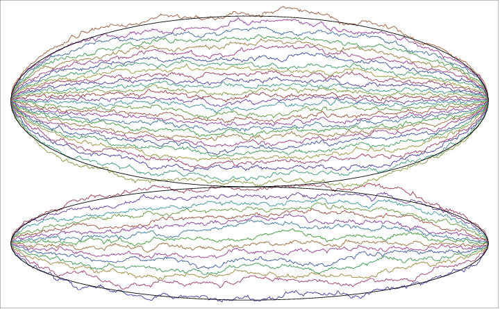
In this paper, we take the $n\to\infty$ limit in the model described above. The global picture is that the two systems of non-colliding Brownian motions form two ellipses touching each other at a tacnode (see Figure 1 for an illustration). Under proper rescaling, we obtain a limiting determinantal point process in the neighborhood of the point of tangency.

Here we consider the general case when two parameters modulate the limit process. One of them is the strength of interaction, called $\sigma$, the other one is a measure of asymmetry, called $\lambda$ which we have chosen to be the ratio of curvatures of the two ellipses at the point of tangency. For $\lambda=1$, we get back to the symmetric case treated in [15].

The scaling of the starting and ending points is

	$\displaystyle a_{1}$	$\displaystyle=-\left(\sqrt{n}+\frac{\sigma}{2}n^{-1/6}\right),$		(1)
	$\displaystyle a_{2}$	$\displaystyle=\sqrt{\lambda}\left(\sqrt{n}+\frac{\sigma}{2}n^{-1/6}\right).$		(2)

We denote by $a$ the distance of the two endpoints:

$$a=a_{2}-a_{1}=\left(1+\sqrt{\lambda}\right)\left(\sqrt{n}+\frac{\sigma}{2}n^{-1/6}\right).$$

(3)

In this setting, the tacnode is at $(1/2,0)$, so that the space-time scaling we need to consider is

	$\displaystyle s$	$\displaystyle=\frac{1}{2}\left(1+\tau_{1}n^{-1/3}\right),$	$\displaystyle t$	$\displaystyle=\frac{1}{2}\left(1+\tau_{2}n^{-1/3}\right),$		(4)
	$\displaystyle u$	$\displaystyle=\frac{1}{2}\xi_{1}n^{-1/6},$	$\displaystyle v$	$\displaystyle=\frac{1}{2}\xi_{2}n^{-1/6}.$

The limiting kernel takes the form

$$\mathcal{L}_{\mathrm{tac}}^{\lambda,\sigma}(\tau_{1},\xi_{1},\tau_{2},\xi_{2})=-\mathbbm{1}(\tau_{1}<\tau_{2})p(\tau_{2}-\tau_{1};\xi_{1},\xi_{2})\\ +L_{\mathrm{tac}}^{\lambda,\sigma}(\tau_{1},\xi_{1},\tau_{2},\xi_{2})+\lambda^{1/6}L_{\mathrm{tac}}^{\lambda^{-1},\lambda^{2/3}\sigma}\left(\lambda^{1/3}\tau_{1},-\lambda^{1/6}\xi_{1},\lambda^{1/3}\tau_{2},-\lambda^{1/6}\xi_{2}\right)$$

(5)

where

$$p(t;x,y)=\frac{1}{\sqrt{4\pi t}}\exp\left(-\frac{(y-x)^{2}}{4t}\right)$$

(6)

is the Gaussian kernel. To describe $L_{\mathrm{tac}}$, we need to introduce some notations. For a parameter $s$, let

$$\operatorname{Ai}^{(s)}(x)=e^{\frac{2}{3}s^{3}+xs}\operatorname{Ai}(s^{2}+x)$$

(7)

be the extended Airy function where $\operatorname{Ai}^{(0)}=\operatorname{Ai}$ is the standard Airy function. The extended Airy kernel is given by

$$K_{\operatorname{Ai}}^{(\alpha,\beta)}(x,y)=\int_{0}^{\infty}\operatorname{Ai}^{(\alpha)}(x+u)\operatorname{Ai}^{(\beta)}(y+u)\,\mathrm{d}u$$

(8)

where $K_{\operatorname{Ai}}^{(0,0)}=K_{\operatorname{Ai}}$ is the standard Airy kernel. Let us denote the function

$$B_{\tau,\xi}^{\lambda}(x)=\int_{0}^{\infty}\operatorname{Ai}^{(\tau)}\left(\xi+\left(1+\sqrt{\lambda^{-1}}\right)^{1/3}\mu\right)\operatorname{Ai}(x+\mu)\mathrm{d}\mu$$

(9)

which is reminiscent of the definition of the Airy kernel. Let also

$$b_{\tau,\xi}^{\lambda}(x)=\lambda^{1/6}\operatorname{Ai}^{(\lambda^{1/3}\tau)}(-\lambda^{1/6}\xi+(1+\sqrt{\lambda})^{1/3}x),$$

(10)

and define

$$L_{\mathrm{tac}}^{\lambda,\sigma}(\tau_{1},\xi_{1},\tau_{2},\xi_{2})=K_{\operatorname{Ai}}^{(-\tau_{1},\tau_{2})}(\sigma+\xi_{1},\sigma+\xi_{2})\\ +(1+\sqrt{\lambda^{-1}})^{1/3}\left\langle B_{\tau_{2},\sigma+\xi_{2}}^{\lambda}-b_{\tau_{2},\sigma+\xi_{2}}^{\lambda},\left(\mathbbm{1}-\chi_{\widetilde{\sigma}}K_{\operatorname{Ai}}\chi_{\widetilde{\sigma}}\right)^{-1}B_{-\tau_{1},\sigma+\xi_{1}}^{\lambda}\right\rangle_{L^{2}((\widetilde{\sigma},\infty))}$$

(11)

where $\chi_{a}(x)=\mathbbm{1}(x>a)$ and

$$\widetilde{\sigma}=\lambda^{1/6}(1+\sqrt{\lambda})^{2/3}\sigma.$$

(12)

Now we can state our main result.

Next we present an alternative formulation of $\mathcal{L}_{\mathrm{tac}}^{\lambda,\sigma}$, inspired from the analogue reformulation of the kernel in [2]. Let us introduce the function

	$\displaystyle C^{\lambda}_{\tau_{,}\xi}(x)$	$\displaystyle=b^{\lambda}_{\tau,\xi}(x)-B^{\lambda}_{\tau,\xi}(x)$		(19)
		$\displaystyle=\lambda^{1/6}\operatorname{Ai}^{(\lambda^{1/3}\tau)}(-\lambda^{1/6}\xi+(1+\sqrt{\lambda})^{1/3}x)$
		$\displaystyle-\int_{0}^{\infty}\operatorname{Ai}^{(\tau)}(\xi+(1+\sqrt{\lambda^{-1}})^{1/3}\mu)\operatorname{Ai}(x+\mu)\mathrm{d}\mu$

Using this definition, we can give another expression for the kernel $\mathcal{L}_{\mathrm{tac}}^{\lambda,\sigma}$ which is formally similar to (5), but the ingredients can be given by a single integral as follows.

In this section, we recall Theorem 1.4 of Johansson in [15], the starting point for our analysis. He obtains a formula for the correlation kernel of two non-colliding families of Brownian particles with the following properties. The first family consists of $n$ particles, and they start at position $a_{1}$ at time $0$ and end at $a_{1}$ at time $1$. The other family has $m$ Brownian motions which start at position $a_{2}$ at time $0$ and end at position $a_{2}$ at time $1$ with $a_{2}>a_{1}$. This system of Brownian motions conditioned on no intersection in the time interval $(0,1)$ forms an extended determinantal point process with kernel $\mathcal{L}_{n,m}(s,u,t,v)$ given as follows.

Let $a=a_{2}-a_{1}$ and $d>0$ a parameter which can be chosen freely in Theorem 2.1. We use the notation

	$\displaystyle\mathcal{A}_{s,u,t,v}^{1}$	$\displaystyle=\frac{d^{2}}{(2\pi i)^{2}\sqrt{(1-s)(1-t)}}\int_{i\mathbb{R}}\mathrm{d}w\int_{D_{a_{1}}}\mathrm{d}z\left(\frac{1-w/a_{1}}{1-z/a_{1}}\right)^{n}\frac{1}{w-z}$		(22)
		$\displaystyle\qquad\times\exp\left(-\frac{sz^{2}}{2(1-s)}-a_{1}z+\frac{uz}{1-s}+\frac{tw^{2}}{2(1-t)}+a_{1}w-\frac{vw}{1-t}\right),$
	$\displaystyle\mathcal{B}_{t,v}^{1}(x)$	$\displaystyle=\frac{d\sqrt{a}}{(2\pi i)^{2}\sqrt{1-t}}\int_{i\mathbb{R}}\mathrm{d}w\int_{D_{a_{1}}}\mathrm{d}z\left(\frac{1-w/a_{1}}{1-z/a_{1}}\right)^{n}\left(1-z/a_{2}\right)^{m}\frac{1}{z-w}$		(23)
		$\displaystyle\qquad\times\exp\left(\frac{tw^{2}}{2(1-t)}+a_{1}w-\frac{vw}{1-t}+axz\right),$
	$\displaystyle\beta_{t,v}^{1}(x)$	$\displaystyle=\frac{d\sqrt{a}}{2\pi i\sqrt{1-t}}\int_{i\mathbb{R}}\mathrm{d}w\left(1-\frac{w}{a_{2}}\right)^{m}\exp\left(\frac{tw^{2}}{2(1-t)}+a_{1}w-\frac{vw}{1-t}+axw\right),$		(24)
	$\displaystyle\mathcal{C}_{s,u}^{1}(y)$	$\displaystyle=\frac{d\sqrt{a}}{(2\pi i)^{2}\sqrt{1-s}}\int_{D_{a_{1}}}\mathrm{d}z\int_{D_{a_{2}}}\mathrm{d}w\left(\frac{1-w/a_{1}}{1-z/a_{1}}\right)^{n}\left(\frac{1}{1-w/a_{2}}\right)^{m}\frac{1}{w-z}$		(25)
		$\displaystyle\qquad\times\exp\left(-\frac{sz^{2}}{2(1-s)}-a_{1}z+\frac{uz}{1-s}-ayw\right),$
	$\displaystyle M_{0}^{1}(x,y)$	$\displaystyle=\frac{a}{(2\pi i)^{2}}\int_{D_{a_{1}}}\mathrm{d}z\int_{D_{a_{2}}}\mathrm{d}w\left(\frac{1-w/a_{1}}{1-z/a_{1}}\right)^{n}\left(\frac{1-z/a_{2}}{1-w/a_{2}}\right)^{m}\frac{1}{z-w}e^{axz-ayw}$		(26)

where $D_{a_{1}}$ and $D_{a_{2}}$ are counterclockwise oriented circles around $a_{1}$ and $a_{2}$ respectively with small radii.

Very similarly, let

	$\displaystyle\mathcal{A}_{s,u,t,v}^{2}$	$\displaystyle=\frac{d^{2}}{(2\pi i)^{2}\sqrt{(1-s)(1-t)}}\int_{i\mathbb{R}}\mathrm{d}w\int_{D_{a_{2}}}\mathrm{d}z\left(\frac{1-w/a_{2}}{1-z/a_{2}}\right)^{m}\frac{1}{w-z}$		(27)
		$\displaystyle\qquad\times\exp\left(-\frac{sz^{2}}{2(1-s)}-a_{2}z+\frac{uz}{1-s}+\frac{tw^{2}}{2(1-t)}+a_{2}w-\frac{vw}{1-t}\right),$
	$\displaystyle\mathcal{B}_{t,v}^{2}(x)$	$\displaystyle=\frac{d\sqrt{a}}{(2\pi i)^{2}\sqrt{1-t}}\int_{i\mathbb{R}}\mathrm{d}w\int_{D_{a_{2}}}\mathrm{d}z\left(1-z/a_{1}\right)^{n}\left(\frac{1-w/a_{2}}{1-z/a_{2}}\right)^{m}\frac{1}{z-w}$		(28)
		$\displaystyle\qquad\times\exp\left(\frac{tw^{2}}{2(1-t)}+a_{2}w-\frac{vw}{1-t}-axz\right),$
	$\displaystyle\beta_{t,v}^{2}(x)$	$\displaystyle=\frac{d\sqrt{a}}{2\pi i\sqrt{1-t}}\int_{i\mathbb{R}}\mathrm{d}w\left(1-\frac{w}{a_{1}}\right)^{n}\exp\left(\frac{tw^{2}}{2(1-t)}+a_{2}w-\frac{vw}{1-t}-axw\right),$		(29)
	$\displaystyle\mathcal{C}_{s,u}^{2}(y)$	$\displaystyle=\frac{d\sqrt{a}}{(2\pi i)^{2}\sqrt{1-s}}\int_{D_{a_{2}}}\mathrm{d}z\int_{D_{a_{1}}}\mathrm{d}w\left(\frac{1}{1-w/a_{1}}\right)^{n}\left(\frac{1-w/a_{2}}{1-z/a_{2}}\right)^{m}\frac{1}{z-w}$		(30)
		$\displaystyle\qquad\times\exp\left(-\frac{sz^{2}}{2(1-s)}-a_{2}z+\frac{uz}{1-s}+ayw\right),$
	$\displaystyle M_{0}^{2}(x,y)$	$\displaystyle=\frac{a}{(2\pi i)^{2}}\int_{D_{a_{2}}}\mathrm{d}z\int_{D_{a_{1}}}\mathrm{d}w\left(\frac{1-z/a_{1}}{1-w/a_{1}}\right)^{n}\left(\frac{1-w/a_{2}}{1-z/a_{2}}\right)^{m}\frac{1}{w-z}e^{-axz+ayw}.$		(31)

Furthermore, let

$$q(s,u,t,v)=\frac{1}{\sqrt{2\pi(t-s)}}\exp\left(-\frac{(u-v)^{2}}{2(t-s)}+\frac{u^{2}}{2(1-s)}-\frac{v^{2}}{2(1-t)}\right)\mathbbm{1}(s<t)$$

(32)

denote the conjugated Brownian kernel.

The theorem below is a consequence of Theorem 1.4 in [15].

First, we give the proof of Theorem 1.1 using two lemmas which are proved in Section 4. We start with formula (33), and we apply it to our present setting. Then, we perform asymptotic analysis for the functions obtained in this way.

The appropriate order of the parameter $d$ is

$$d=\frac{n^{-1/12}}{\sqrt{2}},$$

(35)

since we want $d^{2}\mathcal{L}_{n,\lambda n}$ to converge, so $d^{2}$ is the scaling of the space variables, see (4).

The strategy of the proof is that first, we establish pointwise convergence of the elements of the kernel to the appropriate functions in Lemma 3.1. Then, we give uniform bounds on the functions in Lemma 3.2. This gives, using dominated convergence, that the kernel $\mathcal{L}_{n,\lambda n}$ under the scaling (1)–(4) converges pointwise to $\mathcal{L}_{\mathrm{tac}}^{\sigma,\lambda}$. It turns out that this convergence is uniform on compact sets. Dominated convergence ensures that also the gap probabilities expressed by Fredholm determinants converge.

The following proof is similar to that of Theorem 1.3 in [2], but the idea is adapted to the asymmetric case, so we give it completely.

References

- [1] M. Adler, P.L. Ferrari, and P. van Moerbeke, Non-intersecting random walks in the neighborhood of a symmetric tacnode, arXiv:1007.1163; To appear in Ann. Probab. (2010).
- [2] M. Adler, K. Johansson, and P. van Moerbeke, Double aztec diamonds and the tacnode process, arXiv:1112.5532 (2011).
- [3] J. Ben Hough, M. Krishnapur, Y. Peres, and B. Virág, Determinantal processes and independence, Probability Surveys 3 (2006), 206–229.
- [4] A. Borodin and M. Duits, Limits of determinantal processes near a tacnode, To appear in Ann. Inst. H. Poincaré 47 (2011), 243–258.
- [5] A. Borodin and P.L. Ferrari, Anisotropic growth of random surfaces in dimensions, arXiv:0804.3035 (2008).
- [6] A. Borodin and P.L. Ferrari, Large time asymptotics of growth models on space-like paths I: PushASEP, Electron. J. Probab. 13 (2008), 1380–1418.
- [7] A. Borodin and J. Kuan, Random surface growth with a wall and Plancherel measures for , Comm. Pure Appl. Math. 63 (2010), 831–894.
- [8] S. Delvaux, A. Kuijlaars, and L. Zhang, Critical behavior of non-intersecting Brownian motions at a tacnode, Comm. Pure Appl. Math. 64 (2011), 1305–1383.
- [9] P.L. Ferrari, Polynuclear growth on a flat substrate and edge scaling of GOE eigenvalues, Comm. Math. Phys. 252 (2004), 77–109.
- [10] P.L. Ferrari and H. Spohn, Step fluctations for a faceted crystal, J. Stat. Phys. 113 (2003), 1–46.
- [11] K. Johansson, Non-intersecting paths, random tilings and random matrices, Probab. Theory Related Fields 123 (2002), 225–280.
- [12] K. Johansson, Discrete polynuclear growth and determinantal processes, Comm. Math. Phys. 242 (2003), 277–329.
- [13] K. Johansson, Non-intersecting, simple, symmetric random walks and the extended Hahn kernel, Ann. Inst. Fourier 55 (2005), 2129–2145.
- [14] K. Johansson, Random matrices and determinantal processes, Mathematical Statistical Physics, Session LXXXIII: Lecture Notes of the Les Houches Summer School 2005 (A. Bovier, F. Dunlop, A. van Enter, F. den Hollander, and J. Dalibard, eds.), Elsevier Science, 2006, pp. 1–56.
- [15] K. Johansson, Non-colliding Brownian Motions and the extended tacnode process, arXiv:1105.4027 (2011).
- [16] S. Karlin and L. McGregor, Coincidence probabilities, Pacific J. 9 (1959), 1141–1164.
- [17] M. Katori and H. Tanemura, Symmetry of matrix-valued stochastic processes and noncolliding diffusion particle systems, J. Math. Phys. 45 (2004), 3058–3085.
- [18] M. Katori and H. Tanemura, Infinite systems of noncolliding generalized meanders and Riemann – Liouville differintegrals, Probab. Theory Relat. Fields 138 (2007), 113–156.
- [19] R. Lyons, Determinantal probability measures, Publ. Math. Inst. Hautes Etudes Sci. 98 (2003), 167–212.
- [20] T. Nagao and P.J. Forrester, Multilevel dynamical correlation functions for Dyson’s Brownian motion model of random matrices, Phys. Lett. A 247 (1998), 42–46.
- [21] A. Okounkov and N. Reshetikhin, Correlation function of Schur process with application to local geometry of a random 3-dimensional Young diagram, J. Amer. Math. Soc. 16 (2003), 581–603.
- [22] A. Okounkov and N. Reshetikhin, Random skew plane partitions and the Pearcey process, Comm. Math. Phys. 269 (2007), 571–609.
- [23] M. Prähofer and H. Spohn, Scale invariance of the PNG droplet and the Airy process, J. Stat. Phys. 108 (2002), 1071–1106.
- [24] T. Sasamoto and T. Imamura, Fluctuations of a one-dimensional polynuclear growth model in a half space, J. Stat. Phys. 115 (2004), 749–803.
- [25] A.B. Soshnikov, Determinantal random fields, Encyclopedia of Mathematical Physics (J.-P. Francoise, G. Naber, and T. S. Tsun, eds.), Elsevier, Oxford, 2006, pp. 47–53.
- [26] H. Spohn, Exact solutions for KPZ-type growth processes, random matrices, and equilibrium shapes of crystals, Physica A 369 (2006), 71–99.
- [27] C. Tracy and H. Widom, The Pearcey Process, Comm. Math. Phys. 263 (2006), 381–400.
- [28] C.A. Tracy and H. Widom, Level-spacing distributions and the Airy kernel, Comm. Math. Phys. 159 (1994), 151–174.