跳到论文正文
W Papers独立论文阅读器 arXiv:1112.4883 论文正文 计算阅读时间 · 0%
引用这篇论文根据当前论文元数据生成,正式投稿前建议核对。


License: arXiv.org perpetual non-exclusive license
arXiv:1112.4883v1 [cs.IT] 20 Dec 2011

Computing the Matched Filter in Linear Time
To Solomon Golomb for the occasion of his 80 birthday mazel tov

Alexander Fish Affiliation: Department of Mathematics
University of Wisconsin
Madison, WI 53706, USA
Email: afish@math.wisc.edu
   Shamgar Gurevich Affiliation: Department of Mathematics
University of Wisconsin
Madison, WI 53706, USA
Email: shamgar@math.wisc.edu
   Ronny Hadani Affiliation: Department of Mathematics
University of Texas
Austin, TX 78712, USA
Email: hadani@math.utexas.edu
   Akbar Sayeed Affiliation: Department of Electrical Engineering
University of Wisconsin
Madison, WI 53706, USA
Email: akbar@engr.wisc.edu
   Oded Schwartz Affiliation: Department of Computer Science
University of California
Berkeley, CA 94720, USA
Email: odedsc@eecs.berkeley.edu
Abstract

A fundamental problem in wireless communication is the time-frequency shift (TFS) problem: Find the time-frequency shift of a signal in a noisy environment. The shift is the result of time asynchronization of a sender with a receiver, and of non-zero speed of a sender with respect to a receiver. A classical solution of a discrete analog of the TFS problem is called the matched filter algorithm. It uses a pseudo-random waveform S⁡(t)S(t) of the length p,p, and its arithemtic complexity is O⁡(p2⋅log⁡(p))O(p^{2}\cdot\log(p)), using fast Fourier transform. In these notes we introduce a novel approach of designing new waveforms that allow faster matched filter algorithm. We use techniques from group representation theory to design waveforms S⁡(t),S(t), which enable us to introduce two fast matched filter (FMF) algorithms, called the flag algorithm, and the cross algorithm. These methods solve the TFS problem in O⁡(p⋅log⁡(p))O(p\cdot\log(p)) operations. We discuss applications of the algorithms to mobile communication, GPS, and radar.

I Introduction

Denote by ℋ=ℂ⁡(𝔽p)\mathcal{H}=\mathbb{C}(\mathbb{F}_{p}) the vector space of complex valued functions on the finite field 𝔽p={0,1,…,p−1},\mathbb{F}_{p}=\{0,1,...,p-1\}, where addition and multiplication is done modulo the odd prime number p.p. The vector space ℋ\mathcal{H} is equipped with the standard inner product ⟨f1,f2⟩=∑t∈𝔽pf1​(t)​f2​(t)¯\left\langle f_{1},f_{2}\right\rangle=\mathop{\textstyle\sum}\limits_{t\in\mathbb{F}_{p}}f_{1}(t)\overline{f_{2}(t)}, for f1,f2∈ℋf_{1},f_{2}\in\mathcal{H}, and will be referred to as the Hilbert space of digital signals.

Let us start with a motivational problem.

I-A Mobile communication problem

We consider the following mathematical model of mobile communication [10]. There exists a collection of users j=1,…,rj=1,...,r, each holding a bit bj∈{±1},b_{j}\in\{\pm 1\}, and a private signal Sj∈ℋS_{j}\in\mathcal{H}. User jj transmits its message bj⋅Sjb_{j}\cdot S_{j} to a base station (antenna), and the base station receives the superposition sum

R(t)=∑j=1rbj⋅e2​π​ip​ωj⋅t⋅Sj(t+τj) +𝒲(t), t∈𝔽p,R(t)=\sum_{j=1}^{r}b_{j}\cdot e^{\frac{2\pi i}{p}\omega_{j}\cdot t}\cdot S_{j}(t+\tau_{j})\text{ }+\mathcal{W}(t),\text{ \ \ }t\in\mathbb{F}_{p}, (I.1)

where 𝒲∈ℋ\mathcal{W}\in\mathcal{H} denotes a random white noise of mean zero, τj\tau_{j} encodes the time asynchronization of user jj with the base station, ωj\omega_{j} encodes the radial velocity of user jj with respect to the base station, and i=−1.i=\sqrt{-1}.

The base station ”knows” the signals SjS_{j}’s and RR. The objective is:

Problem I.1 (Mobile communication problem)

Extract the bits bj,b_{j}, j=1,…,r.j=1,...,r.

A resolution of Problem I.1 will be deduced (see Section I-F) from our solution to the following problem.

I-B The time-frequency shift (TFS) problem

We have rr signals Sj∈ℋS_{j}\in\mathcal{H}, j=1,…,r,j=1,...,r, called the sender waveforms. Additionally, we are given the receiver waveform R∈ℋR\in\mathcal{H}, which satisfies

R(t)=∑j=1re2​π​ip​ωj⋅t⋅Sj(t+τj) +𝒲(t), t∈𝔽p,R(t)=\sum_{j=1}^{r}e^{\frac{2\pi i}{p}\omega_{j}\cdot t}\cdot S_{j}(t+\tau_{j})\text{ }+\mathcal{W}(t),\text{ \ \ }t\in\mathbb{F}_{p}, (I.2)

where 𝒲∈ℋ\mathcal{W}\in\mathcal{H} denotes a random white noise of mean zero, and (τj,ωj)∈𝔽p×𝔽p\left(\tau_{j},\omega_{j}\right)\in\mathbb{F}_{p}\times\mathbb{F}_{p}, j=1,…,r.j=1,...,r. We will call the pairs (τj,ωj)\left(\tau_{j},\omega_{j}\right) the time-frequency shifts, and the vector space V=𝔽p×𝔽pV=\mathbb{F}_{p}\times\mathbb{F}_{p} the time-frequency plane.

The precise formulation of the time-frequency shift problem is the following:

Problem I.2 (TFS problem)

Given the waveforms Sj,S_{j}, j=1,…,r,j=1,...,r, and R,R, extract the time-frequency shifts (τj,ωj)∈V\left(\tau_{j},\omega_{j}\right)\in V, j=1,…,r.j=1,...,r.

I-C The matched filter (MF) algorithm

A classical solution [3, 4, 5, 7, 10, 11, 12] to Problem I.2, is the matched filter algorithm. For a fixed k∈{1,…,r},k\in\{1,...,r\}, we define the following matched filter (MF) matrix of the sender SkS_{k}, and the receiver RR:

ℳ⁡[Sk,R]​(τ,ω)=⟨e2​π​ip​ω⋅t⋅Sk​(t+τ),R⁡(t)⟩,(τ,ω)∈V.\mathcal{M}[S_{k},R](\tau,\omega)=\left\langle e^{\frac{2\pi i}{p}\omega\cdot t}\cdot S_{k}(t+\tau),R(t)\right\rangle,\ \ (\tau,\omega)\in V. (I.3)

A direct verification shows that for ζj=e2​π​ip​(τ​ωj−ω​τj)\zeta_{j}=e^{\frac{2\pi i}{p}(\tau\omega_{j}-\omega\tau_{j})}, j=1,…,rj=1,...,r, we have

ℳ​[Sk,R]​(τ,ω)\displaystyle\mathcal{M}[S_{k},R](\tau,\omega) =\displaystyle= ζk⋅ℳ⁡[Sk,Sk]​(τ−τk,ω−ωk)\displaystyle\zeta_{k}\cdot\mathcal{M}[S_{k},S_{k}](\tau-\tau_{k},\omega-\omega_{k}) (I.4)
+∑j≠kζj⋅ℳ[Sk,Sj](τ−τj,ω−ωj)\displaystyle+\sum_{j\neq k}\zeta_{j}\cdot\mathcal{M[}S_{k},S_{j}](\tau-\tau_{j},\omega-\omega_{j})
+O⁡(N​S​Rp),\displaystyle+O(\frac{NSR}{\sqrt{p}}),

where N​S​R=1S​N​RNSR=\frac{1}{SNR} is the inverse of the signal-to-noise ratio between the waveform SkS_{k} and 𝒲.\mathcal{W}. For simplicity, we assume that the N​S​RNSR is not too large, and, for the rest of the paper, we will omit the last term in (I.4).

In order to extract the time-frequency shift (τk,ωk),(\tau_{k},\omega_{k}), using the matched filter, it is ”standard” (see [3, 4, 5, 7, 10, 11, 12]) to use almost-orthogonal pseudo-random signals Sj∈ℋS_{j}\in\mathcal{H} of norm one. Namely, all the summands in right-hand side of (I.4) are of size O⁡(1p)O(\frac{1}{\sqrt{p}}), with the exception that for (τ,ω)=(τk,ωk)(\tau,\omega)=(\tau_{k},\omega_{k}) we have ℳ⁡[Sk,Sk]​(τ−τk,ω−ωk)=1.\mathcal{M}[S_{k},S_{k}](\tau-\tau_{k},\omega-\omega_{k})=1. Hence,

|ℳ⁡[Sk,R]​(τ,ω)|={1+εr,p​, if ​(τ,ω)=(τk,ωk);εr,p​, if ​(τ,ω)≠(τk,ωk),\left|\mathcal{M}[S_{k},R](\tau,\omega)\right|=\left\{\begin{array}[]{c}1+\varepsilon_{r,p}\text{, if }(\tau,\omega)=(\tau_{k},\omega_{k});\\ \varepsilon_{r,p}\text{, \ \ \ \ \ if }(\tau,\omega)\neq(\tau_{k},\omega_{k}),\end{array}\right. (I.5)

where εr,p=O⁡(rp).\varepsilon_{r,p}=O(\frac{r}{\sqrt{p}}).

Refer to caption
Fig. 1: |ℳ⁡[S1,R]|\left|\mathcal{M}[S_{1},R]\right| with pseudo-random S1,S2S_{1},S_{2}, and (τ1,ω1)=(50,50)(\tau_{1},\omega_{1})=(50,50)

Identity (I.5) suggests the following ”entry-by-entry” algorithmic solution to TFS problem: Compute the matrix ℳ⁡[Sk,R],\mathcal{M}[S_{k},R], and choose (τk,ωk)(\tau_{k},\omega_{k}) for which |ℳ⁡[Sk,R]​(τk,ωk)|≈1.\left|\mathcal{M}[S_{k},R](\tau_{k},\omega_{k})\right|\approx 1. However, this solution of TFS problem is very expensive in terms of arithmetic complexity, i.e., the number of arithmetic (multiplication, and addition) is O⁡(r⋅p3).O(r\cdot p^{3}). One can do better using a ”line-by-line” computation. This is due to the next observation.

Remark I.3 (FFT)

The restriction of the matrix ℳ⁡[Sk,R]\mathcal{M[}S_{k},R] to any line (not necessarily through the origin) in the time-frequency plane V,V, is a convolution that can be computed, using the fast Fourier transform algorithm (FFT), in O⁡(p⋅log⁡(p))O(p\cdot\log(p)) arithmetic operations.

As a consequence of Remark I.3, one can solve TFS problem in O⁡(r⋅p2⋅log⁡(p))O(r\cdot p^{2}\cdot\log(p)) arithmetic operations. To the best of our knowledge, the ”line-by-line” computation is also the fastest method which exists in the literature [9]. Note that computing one entry in ℳ⁡[Sk,R]\mathcal{M[}S_{k},R] costs already O⁡(p)O(p) operations. This leads to the following fast matched filter (FMF) problem:

Problem I.4 (FMF problem)

Design waveforms Sj∈ℋS_{j}\in\mathcal{H}, j=1,…,r,j=1,...,r, to solve TFS problem in almost linear time for shift.

I-D The flag method

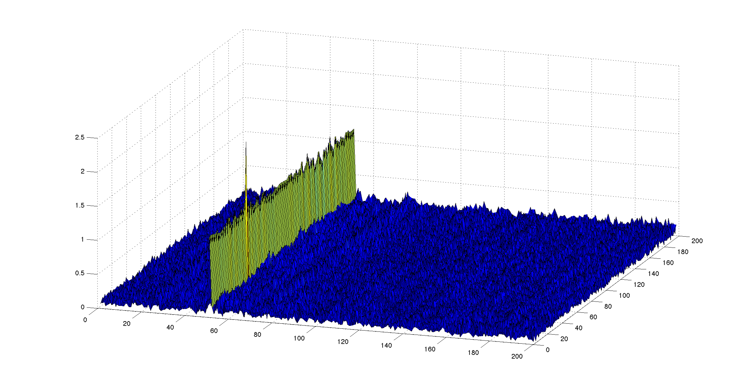
We introduce the flag method to propose a solution to FMF problem. We will show how to associate with the p+1p+1 lines, through (0,0)(0,0) in the time-frequency plane, Lj,L_{j}, j=1,…,p+1,j=1,...,p+1, a system of almost orthogonal waveforms SLj∈ℋ,S_{L_{j}}\in\mathcal{H}, that we will call flags. The system satisfies

|ℳ⁡[SLk,R]​(τ,ω)|={2+εr,p, if (τ,ω)=(τk,ωk); 1+εr,p​, if ​(τ,ω)∈Lk′∖(τk,ωk);εr,p, if (τ,ω)∈V∖Lk′, \left|\mathcal{M}[S_{L_{k}},R](\tau,\omega)\right|=\left\{\begin{array}[]{c}2+\varepsilon_{r,p}\text{, \ if }(\tau,\omega)=(\tau_{k},\omega_{k});\text{ \ \ \ \ \ \ \ }\\ 1+\varepsilon_{r,p}\text{, \ if }(\tau,\omega)\in L_{k}^{\prime}\smallsetminus(\tau_{k},\omega_{k});\\ \varepsilon_{r,p}\text{,\ \ if }(\tau,\omega)\in V\smallsetminus L_{k}^{\prime},\text{\ \ \ \ \ \ \ \ \ \ \ \ \ \ \ }\end{array}\right. (I.6)

where εr,p=O⁡(rp),\varepsilon_{r,p}=O(\frac{r}{\sqrt{p}}), RR is the receiver waveform (I.2), defined with respect to any rr flags containing SLk,S_{L_{k}}, and Lk′L_{k}^{\prime} is the shifted line Lk+(τk,ωk)L_{k}+(\tau_{k},\omega_{k}).

Refer to caption
Fig. 2: |M⁡[SL1,R]|\left|M[S_{L_{1}},R]\right| with two flags SL1,SL2S_{L_{1}},S_{L_{2}}, and (τ1,ω1)=(50,50)(\tau_{1},\omega_{1})=(50,50)

Identity (I.6) suggests the ”flag” algorithmic solution to FMF problem in the case that the number of waveforms r≪p,r\ll\sqrt{p}, and pp is sufficiently large. In the following we assume that RR and SLkS_{L_{k}} are as in (I.6).

Algorithm I.5 (Flag algorithm)
  • •

    Choose a line Lk⊥L_{k}^{\bot} different from Lk.L_{k}.

  • •

    Compute ℳ⁡[SLk,R]\mathcal{M}[S_{L_{k}},R] on Lk⊥L_{k}^{\bot}. Find (τ,ω)(\tau,\omega) such that |ℳ⁡[SLk,R]​(τ,ω)|\left|\mathcal{M}[S_{L_{k}},R](\tau,\omega)\right| ≈1\approx 1, i.e., (τ,ω)(\tau,\omega) on the shifted line Lk+(τk,ωk).L_{k}+(\tau_{k},\omega_{k}).

  • •

    Compute ℳ⁡[SLk,R]\mathcal{M}[S_{L_{k}},R] on Lk+(τk,ωk)L_{k}+(\tau_{k},\omega_{k}) and find (τ,ω)(\tau,\omega) such that |ℳ⁡[SLk,R]​(τ,ω)|≈2.\left|\mathcal{M}[S_{L_{k}},R](\tau,\omega)\right|\approx 2.\vskip 3.0pt plus 1.0pt minus 1.0pt

The arithmetic complexity of the flag algorithm is O⁡(r⋅p​log⁡(p)),O(r\cdot p\log(p)), using the FFT (Remark I.3).

Refer to caption
Fig. 3: Diagram of the flag algorithm

I-E The cross method

Another solution to the TFS problem, and subsequently to the mobile communication problem, is the cross method. The idea is similar to the flag method, i.e., first to find a line on which the time-frequency shift is located, and then to search on the line to find the time-frequency shift. We will show how to associate with the p+12\frac{p+1}{2} distinct pairs of lines L,M⊂VL,M\subset V a system of almost-orthogonal waveforms SL,M,S_{{}_{L},_{M}}, that we will call crosses. The system satisfies

|ℳ[SL,M,R]|={2+εr,p, if (τ,ω)=(τL,M,ωL,M); 1+εr,p, if (τ,ω)∈(L′∪M′)∖(τL,M,ωL,M);εr,p​, if ​(τ,ω)∈V∖(L′∪M′), \left|\mathcal{M[}S_{{}_{L},_{M}},R\mathcal{]}\right|{\small=}\left\{\begin{array}[]{c}{}_{2+\varepsilon_{r,p}\text{, \ if }(\tau,\omega)=(\tau_{{}_{L},_{M}},\omega_{{}_{L},_{M}});}\text{ \ \ \ \ \ \ \ \ \ }\\ {}_{1+\varepsilon_{r,p}\text{, \ if }(\tau,\omega)\in(L^{\prime}\cup M^{\prime})\smallsetminus(\tau_{{}_{L},_{M}},\omega_{{}_{L},_{M}});}\\ {}_{\varepsilon_{r,p}\text{,\ \ if }(\tau,\omega)\in V\smallsetminus(L^{\prime}\cup M^{\prime}),}\text{\ \ \ \ \ \ \ \ \ \ \ \ \ \ \ \ \ }\end{array}\right.

where εr,p=O⁡(rp),\varepsilon_{r,p}=O(\frac{r}{\sqrt{p}}), RR is the receiver waveform (I.2), defined with respect to any rr different crosses containing SL,M,S_{{}_{L},_{M}}, and L′=L+(τL,M,ωL,M)L^{\prime}=L+(\tau_{{}_{L},_{M}},\omega_{{}_{L},_{M}}), M′=M+(τL,M,ωL,M).M^{\prime}=M+(\tau_{{}_{L},_{M}},\omega_{{}_{L},_{M}}).

Refer to caption
Fig. 4: |ℳ[SL1,M1,R]||\mathcal{M}[S_{{}_{L_{1}},_{M_{1}}},R]| with crosess SL1,M1,SL2,M2S_{{}_{L_{1}},_{M_{1}}},S_{{}_{L_{2}},_{M_{2}}}, and (τ1,ω1)=(50,50)(\tau_{1},\omega_{1})=(50,50)

The arithmetic complexity of the cross method is O⁡(r⋅p​log⁡(p)),O(r\cdot p\log(p)), using the FFT (Remark I.3).

I-F Solution to the mobile communication problem

Looking back to Problem I.1, we see that the flag and cross algorithms suggest a fast O⁡(r⋅p⋅log⁡(p))O(r\cdot p\cdot\log(p)) solution to extract ALL the bits bk.b_{k}. Indeed, identity (I.4) implies that bk≈ℳ⁡[Sk,R]​(τk,ωk)/2,b_{k}\approx\mathcal{M}[S_{k},R](\tau_{k},\omega_{k})/2, k=1,…,r,k=1,...,r, where RR is the waveform (I.1), with Sj=SLjS_{j}=S_{L_{j}}, j=1,…,rj=1,...,r, for the flag method, or Sj=SLj,MjS_{j}=S_{{}_{L_{j}},_{M_{j}}}, j=1,…,rj=1,...,r, for the cross method, and r≪p.r\ll\sqrt{p}.

II The Heisenberg–Weil flag system

The flag waveforms, that play the main role in the flag algorithm, are of a special form. Each of them is a sum of a pseudorandom signal and a structural signal. The first has the MF matrix which is almost delta function at the origin, and the MF matrix of the second is supported on a line. The designs of these waveforms are done using group representation theory. The pseudorandom signals are designed [4, 5, 12] using the Weil representation, and will be called Weil (peak) signals11 1 For the purpose of the Flag method, other pseudorandom signals may work.. The structural signals are designeded [6, 7] using the Heisenberg representation, and will be called Heisenberg (lines) signals. We will call the collection of all flag waveforms, the Heisenberg–Weil flag system. In this section we briefly recall constructions, and properties of these waveforms. A more comprehensive treatment, including proofs, will appear in [2].

II-A The Heisenberg (lines) system

Consider the following collection of unitary operators, called Heisenberg operators, that act on the Hilbert space of digital signals:

{π(τ,ω):ℋ→ℋ, τ,ω∈𝔽p;π⁡(τ,ω)=Mω∘Lτ, \left\{\begin{array}[]{c}\pi(\tau,\omega):\mathcal{H\rightarrow\mathcal{H}},\text{ \ }\tau,\omega\in\mathbb{F}_{p};\\ \pi(\tau,\omega)=\mathrm{M}_{\omega}\circ\mathrm{L}_{\tau},\end{array}\right.\text{ \ \ \ \ \ \ \ \ \ \ \ \ \ \ } (II.1)

where Lτ​[f]​(t)=f⁡(t+τ)\mathrm{L}_{\tau}[f](t)=f(t+\tau) is the time-shift operator, Mω​[f]​(t)=e2​π​ip​ω⋅t⋅f⁡(t)\mathrm{M}_{\omega}[f](t)=e^{\frac{2\pi i}{p}\omega\cdot t}\cdot f(t) is the frequency-shift operator, for every f∈ℋf\in\mathcal{H}, t∈𝔽p,t\in\mathbb{F}_{p}, and ∘\circ denotes composition of operators.

The operators (II.1) do not commute in general, but rather obey the Heisenberg commutation relations π⁡(τ,ω)∘π⁡(τ′,ω′)=e2​π​ip​(τ​ω′−ω​τ′)⋅π⁡(τ′,ω′)∘π⁡(τ,ω).\pi(\tau,\omega)\circ\pi(\tau^{\prime},\omega^{\prime})=e^{\frac{2\pi i}{p}(\tau\omega^{\prime}-\omega\tau^{\prime})}\cdot\pi(\tau^{\prime},\omega^{\prime})\circ\pi(\tau,\omega). The expression τ​ω′−ω​τ′\tau\omega^{\prime}-\omega\tau^{\prime} vanishes if (τ,ω)(\tau,\omega), (τ′,ω′)(\tau^{\prime},\omega^{\prime}) belong to the same line. Hence, for a given line L⊂V=𝔽p×𝔽pL\subset V=\mathbb{F}_{p}\times\mathbb{F}_{p} we have a commutative collection of unitary operators

π(ℓ):ℋ→ℋ, ℓ∈L.\pi(\ell):\mathcal{H\rightarrow\mathcal{H}},\text{ }\ell\in L. (II.2)

We use the theorem from linear algebra about simultaneous diagonalization of commuting unitary operators, and obtain [6, 7] a natural orthonormal basis ℬL ⊂ℋ\mathcal{B}_{L\text{ }}\subset\mathcal{H} consisting of common eigenfunctions for all the operators (II.2). The system of all such bases ℬL,\mathcal{B}_{L}, where LL runs over all lines through the origin in V,V, will be called the Heisenberg (lines) system. We will need the following result [6, 7]:

Theorem II.1

The Heisenberg system satisfies the properties

  1. 1.

    Line. For every line L⊂VL\subset V, and every fL∈ℬLf_{L}\in\mathcal{B}_{L}, we have

    |ℳ⁡[fL,fL]​(τ,ω)|={1, if ​(τ,ω)∈L;0, if ​(τ,ω)∉L.\left|\mathcal{M}[f_{L},f_{L}](\tau,\omega)\right|=\left\{\begin{array}[]{c}1,\text{ if }\left(\tau,\omega\right)\in L;\\ 0,\text{ if }\left(\tau,\omega\right)\notin L.\end{array}\right.
  2. 2.

    Almost-orthogonality. For every two lines L1≠L2⊂VL_{1}\neq L_{2}\subset V, and every fL1∈ℬL1f_{L_{1}}\in\mathcal{B}_{L_{1}}, fL2∈ℬL2,f_{L_{2}}\in\mathcal{B}_{L_{2}}, we have

    |ℳ[fL1,fL2](τ,ω)|=1p, \left|\mathcal{M}[f_{L_{1}},f_{L_{2}}](\tau,\omega)\right|=\frac{1}{\sqrt{p}},\text{ \ }

    for every (τ,ω)∈V.(\tau,\omega)\in V.

Refer to caption
Fig. 5: |ℳ⁡[fL,fL]|\left|\mathcal{M}[f_{L},f_{L}]\right| for L={(τ,τ);L=\{(\tau,\tau); τ∈𝔽p}\tau\in\mathbb{F}_{p}\}

II-B The Weil (peaks) system

Consider the following collection of matrices

G=SL2(𝔽p)={(abcd); a,b,c,d∈𝔽p, and ad−bc=1}.G=SL_{2}(\mathbb{F}_{p})=\left\{\begin{pmatrix}a&b\\ c&d\end{pmatrix};\text{ }a,b,c,d\in\mathbb{F}_{p},\text{ and }ad-bc=1\right\}.

Note that GG is in a natural way a group [1] with respect to the operation of matrix multiplication. It is called the special linear group of order two over 𝔽p.\mathbb{F}_{p}. Each element g∈Gg\in G acts on the time-frequency plane VV via the change of coordinates v↦g⋅v.v\mapsto g\cdot v. For every g∈Gg\in G, let ρ⁡(g)\rho(g) be a linear operator on ℋ\mathcal{H} which is a solution of the following system of p2p^{2} linear equations:

Σg: ρ(g)∘π(τ,ω)=π(g⋅(τ,ω))∘ρ(g), τ,ω∈𝔽p,\Sigma_{g}:\text{ }\rho(g)\circ\pi(\tau,\omega)=\pi(g\cdot(\tau,\omega))\circ\rho(g),\text{\ \ }\tau,\omega\in\mathbb{F}_{p}, (II.3)

where π\pi is defined by (II.1). Denote by Sol⁡(Σg)\mathrm{Sol}(\Sigma_{g}) the space of all solutions to System (II.3). The following is a basic result [13]:

Theorem II.2 (Stone–von Neumann–Schur-Weil)

There exist a unique collection of solutions {ρ(g)∈Sol(Σg);\{\rho(g)\in\mathrm{Sol}(\Sigma_{g}); g∈G},g\in G\}, which are unitary operators, and satisfy the homomorphism condition ρ⁡(g⋅h)=ρ⁡(g)∘ρ⁡(h).\rho(g\cdot h)=\rho(g)\circ\rho(h).\vskip 3.0pt plus 1.0pt minus 1.0pt

Denote by U⁡(ℋ)U(\mathcal{H)} the collection of all unitary operators on the Hilbert space of digital signals ℋ\mathcal{H}. Theorem II.2 establishes the map ρ:G→U⁡(ℋ)\rho:G\rightarrow U(\mathcal{H}), which is called the Weil representation [13]. The group GG is not commutative, but contains a special class of maximal commutative subgroups called tori22 2 There are order of p2p^{2} tori in S​L2​(𝔽p).SL_{2}(\mathbb{F}_{p}). [4, 5]. Each torus T⊂GT\subset G acts via the Weil representation operators

ρ⁡(g):ℋ→ℋ​, ​g∈T.\rho(g):\mathcal{H\rightarrow\mathcal{H}}\text{, \ }g\in T. (II.4)

This is a commutative collection of diagonalizable operators, and it admits [4, 5] a natural orthonormal basis ℬT\mathcal{B}_{T} for ℋ\mathcal{H}, consisting of common eigenfunctions. The system of all such bases ℬT,\mathcal{B}_{T}, where TT runs over all tori in G,G, will be called the Weil (peaks) system. We will need the following result [4, 5]:

Theorem II.3

The Weil system satisfies the properties

  1. 1.

    Peak. For every torus T⊂GT\subset G, and every φT∈ℬT\varphi_{T}\in\mathcal{B}_{T}, we have

    |ℳ⁡[φT,φT]​(τ,ω)|={1, if ​(τ,ω)=(0,0);≤2p, if (τ,ω)≠(0,0).\left|\mathcal{M}[\varphi_{T},\varphi_{T}](\tau,\omega)\right|=\left\{\begin{array}[]{c}1,\text{ if }\left(\tau,\omega\right)=(0,0);\\ \leq\frac{2}{\sqrt{p}},\text{ if }\left(\tau,\omega\right)\neq(0,0).\end{array}\right.
  2. 2.

    Almost-orthogonality. For every two tori T1,T_{1}, T2⊂GT_{2}\subset G, and every φT1∈ℬT1\varphi_{T_{1}}\in\mathcal{B}_{T_{1}}, φT2∈ℬT2,\varphi_{T_{2}}\in\mathcal{B}_{T_{2}}, with φT1≠φT2,\varphi_{T_{1}}\neq\varphi_{T_{2}}, we have

    |ℳ[φT1,φT2](τ,ω)|≤{4p, if ​T1≠T2;2p, if ​T1=T2, \left|\mathcal{M}[\varphi_{T_{1}},\varphi_{T_{2}}](\tau,\omega)\right|\leq\left\{\begin{array}[]{c}\frac{4}{\sqrt{p}},\text{ if }T_{1}\neq T_{2};\\ \frac{2}{\sqrt{p}},\text{ if }T_{1}=T_{2},\end{array}\right.\text{ \ }

    for every (τ,ω)∈V.(\tau,\omega)\in V.

Refer to caption
Fig. 6: ℳ⁡[φT,φT]\mathcal{M}[\varphi_{T},\varphi_{T}] for T={(a00a−1);0≠a∈𝔽p}T=\{\begin{pmatrix}a&0\\ 0&a^{-1}\end{pmatrix};0\neq a\in\mathbb{F}_{p}\}

II-C The Heisenberg–Weil system

We define the Heisenberg–Weil system of waveforms. This is the collection of signals in ℋ\mathcal{H}, which are of the form SL=fL+φTS_{L}=f_{L}+\varphi_{T}, where fLf_{L} and φT\varphi_{T} are Heisenberg and Weil waveforms, respectively. The main technical result of this paper is:

Theorem II.4

The Heisenberg–Weil system satisfies the properties

  1. 1.

    Flag. For every line L⊂VL\subset V, torus T⊂GT\subset G, and every flag SL=fL+φT,S_{L}=f_{L}+\varphi_{T}, with fL∈ℬL,f_{L}\in\mathcal{B}_{L}, φT∈ℬT\varphi_{T}\in\mathcal{B}_{T}, we have

    |ℳ⁡[SL,SL]​(τ,ω)|={2+ϵp, if (τ,ω)=(0,0); 1+εp, if (τ,ω)∈L∖(0,0);  εp, if (τ,ω)∈V∖L, \left|\mathcal{M}[S_{L},S_{L}](\tau,\omega)\right|=\left\{\begin{array}[]{c}2+\epsilon_{p}\text{, \ if }(\tau,\omega)=(0,0);\text{ \ \ \ \ \ \ \ }\\ 1+\varepsilon_{p}\text{, \ if }(\tau,\omega)\in L\smallsetminus(0,0);\text{ \ \ }\\ \text{ }\varepsilon_{p}\text{, \ if }(\tau,\omega)\in V\smallsetminus L,\text{\ \ \ \ \ \ \ \ \ \ \ \ \ \ \ \ }\end{array}\right.

    where |ϵp|≤4p,|\epsilon_{p}|\leq\frac{4}{\sqrt{p}}, and |εp|≤6p.|\varepsilon_{p}|\leq\frac{6}{\sqrt{p}}.

  2. 2.

    Almost-orthogonality. For every two lines L1≠L2⊂VL_{1}\neq L_{2}\subset V, tori T1,T_{1}, T2⊂G,T_{2}\subset G, and every two flags SLj=fLj+φTj,S_{L_{j}}=f_{L_{j}}+\varphi_{T_{j}}, with fLj∈ℬLjf_{L_{j}}\in\mathcal{B}_{L_{j}}, φTj∈ℬTj\varphi_{T_{j}}\in\mathcal{B}_{T_{j}}, j=1,2,j=1,2, φT1≠φT2,\varphi_{T_{1}}\neq\varphi_{T_{2}}, we have

    |ℳ[SL1,SL2](τ,ω)|≤{9p, if ​T1≠T2;7p, if ​T1=T2, \left|\mathcal{M}[S_{L_{1}},S_{L_{2}}](\tau,\omega)\right|\leq\left\{\begin{array}[]{c}\frac{9}{\sqrt{p}},\text{ if }T_{1}\neq T_{2};\\ \frac{7}{\sqrt{p}},\text{ if }T_{1}=T_{2},\end{array}\right.\text{ \ }

    for every (τ,ω)∈V.(\tau,\omega)\in V.

A proof of Theorem II.4 will appear in [2].

Refer to caption
Fig. 7: |ℳ⁡[SL,SL]|\left|\mathcal{M}[S_{L},S_{L}]\right| for Heisenberg–Weil flag with L={(τ,τ);L=\{(\tau,\tau); τ∈𝔽p}\tau\in\mathbb{F}_{p}\}
Remark II.5

As a consequence of Theorem II.4 we obtain families of p+1p+1 almost-orthogonal flag waveforms which can be used for solving the TFS and mobile communication problems in almost linear time.

III The Heisenberg cross system

We define the Heisenberg cross system of waveforms. This is the collection of signals in ℋ\mathcal{H}, which are of the form SL,M=fL+fMS_{{}_{L},_{M}}=f_{L}+f_{M}, where fL,fM,f_{L},f_{M}, L≠M,L\neq M, are Heisenberg waveforms defined in Section II-A. The following follows immediately from Theorem II.1:

Theorem III.1

The Heisenberg cross system satisfies the properties

  1. 1.

    Cross. For every pair of distinct lines L,M⊂VL,M\subset V, and every cross SL,M=fL+fMS_{{}_{L},_{M}}=f_{L}+f_{M}, with fL∈ℬL,f_{L}\in\mathcal{B}_{L}, fM∈ℬMf_{M}\in\mathcal{B}_{M}, we have

    |ℳ[SL,M,SL,M](τ,ω)|={2+εp​, if ​(τ,ω)=(0,0); 1+εp​, if ​(τ,ω)∈(L∪M)∖(0,0);  εp​, if ​(τ,ω)∈V∖(L∪M), \left|\mathcal{M}[S_{{}_{L},_{M}},S_{{}_{L},_{M}}](\tau,\omega)\right|=\left\{\begin{array}[]{c}{}_{2+\varepsilon_{p}\text{, \ if }(\tau,\omega)=(0,0);}\text{ \ \ \ \ \ \ \ \ \ \ \ \ \ \ \ \ }\\ {}_{1+\varepsilon_{p}\text{, \ if }(\tau,\omega)\in(L\cup M)\smallsetminus(0,0);}\text{ \ \ \ \ \ \ \ }\\ \text{ }_{\varepsilon_{p}\text{, \ if }(\tau,\omega)\in V\smallsetminus(L\cup M),}\text{\ \ \ \ \ \ \ \ \ \ \ \ \ \ \ }\end{array}\right.

    where |εp|≤2p.|\varepsilon_{p}|\leq\frac{2}{\sqrt{p}}.

  2. 2.

    Almost-orthogonality. For every four distinct lines L1,M1,L2,M2⊂VL_{1},M_{1},L_{2},M_{2}\subset V, and every two crosses SLj,Mj=fLj+fMj,S_{{}_{L_{j}},_{M_{j}}}=f_{L_{j}}+f_{M_{j}}, j=1,2,j=1,2, we have

    |ℳ[SL1,M1,SL2,M2](τ,ω)|≤4p. \left|\mathcal{M}[S_{{}_{L_{1}},_{M_{1}}},S_{{}_{L_{2}},_{M_{2}}}](\tau,\omega)\right|\leq\frac{4}{\sqrt{p}}.\text{\ }

    for every (τ,ω)∈V.(\tau,\omega)\in V.

Remark III.2

As a consequence of Theorem III.1 we obtain families of p+12\frac{p+1}{2} almost-orthogonal cross waveforms which can be used for solving the TFS and mobile communication problems in almost linear time.

IV Applications to GPS and radar

In the introduction we described application of flag and cross methods to mobile communication. In this section we demonstrate applications to global positioning system (GPS), and discrete radar.

IV-A Application to global positioning system (GPS)

The model of GPS works as follows [8]. A client on the earth surface wants to know his geographical location. Satellites j=1,…,rj=1,...,r send to earth their location. For simplicity, the location of satellite jj is a bit bj∈{±1}.b_{j}\in\{\pm 1\}. Satellite jj transmits to the earth its signal Sj∈ℋS_{j}\in\mathcal{H} multiplied by its location bj.b_{j}. The client receives the signal

R(t)=∑j=1rbj⋅e2​π​ip​ωj⋅t⋅Sj(t+τj) +𝒲(t),R(t)=\sum_{j=1}^{r}b_{j}\cdot e^{\frac{2\pi i}{p}\omega_{j}\cdot t}\cdot S_{j}(t+\tau_{j})\text{ }+\mathcal{W}(t),

where ωj\omega_{j} encodes the radial velocity of satellite jj with respect to the client, τj\tau_{j} encodes the distance between satellite jj and the client33 3 From the τj\tau_{j} we can find [8] the distance between satellite jj and the client, given that r≥4r\geq 4 and the clocks of all satellites are synchronized., and 𝒲\mathcal{W} is a random white noise of mean zero.

Problem IV.1 (GPS problem)

Find (bj,τj),(b_{j},\tau_{j}), j=1,…,r.j=1,...,r.

By using Heisenberg–Weil or Heisenberg cross waveforms we find the pairs (bj,τj)(b_{j},\tau_{j}) in O⁡(r⋅p​log⁡(p))O(r\cdot p\log(p)) arithmetical operations.

IV-B Application to discrete radar

The model of discrete radar works as follows [7]. A radar sends a waveform S∈ℋS\in\mathcal{H} which bounds back by rr targets. The signal R∈ℋR\in\mathcal{H} which is received as an echo has the form44 4 In practice there are intensity coefficients 0≤αj≤10\leq\alpha_{j}\leq 1 such that R⁡(t)=∑j=1rαj⋅e2​π​ip​ωj⋅t⋅S⁡(t+τj)R(t)=\sum_{j=1}^{r}\alpha_{j}\cdot e^{\frac{2\pi i}{p}\omega_{j}\cdot t}\cdot S(t+\tau_{j}) +𝒲⁡(t).+\mathcal{W}(t). Assuming that αj\alpha_{j}’s are sufficiently large our methods are applicable verbatim.

R(t)=∑j=1re2​π​ip​ωj⋅t⋅S(t+τj) +𝒲(t),R(t)=\sum_{j=1}^{r}e^{\frac{2\pi i}{p}\omega_{j}\cdot t}\cdot S(t+\tau_{j})\text{ }+\mathcal{W}(t),

where ωj\omega_{j} encodes the radial velocity of target jj with respect to the radar, τj\tau_{j} encodes the distance between target jj and the radar, and 𝒲\mathcal{W} is a random white noise of mean zero.

Problem IV.2 (Discrete radar problem)

Find (τj,ωj),(\tau_{j},\omega_{j}), j=1,…,r.j=1,...,r.\vskip 3.0pt plus 1.0pt minus 1.0pt\vskip 3.0pt plus 1.0pt minus 1.0pt

By sending Heisenberg–Weil waveform SL=fL+φTS_{L}=f_{L}+\varphi_{T} we get55 5 For simplicity we assume that all the shifted lines L+(τj,ωj)L+(\tau_{j},\omega_{j})’s are distinct. The general case is treated similarly.

|ℳ⁡[SL,R]​(τ,ω)|={2+εr,p, if (τ,ω)∈{(τj,ωj)}; 1+εr,p, if (τ,ω)∈L+(τj,ωj)∖(τj,ωj); εr,p​, otherwise, \left|\mathcal{M}[S_{L},R](\tau,\omega)\right|=\left\{\begin{array}[]{c}2+\varepsilon_{r,p}\text{, if }(\tau,\omega)\in\{(\tau_{j},\omega_{j})\};\text{ \ \ \ \ \ \ \ \ \ \ \ \ \ \ \ \ \ }\\ 1+\varepsilon_{r,p}\text{, if }(\tau,\omega)\in L+(\tau_{j},\omega_{j})\smallsetminus(\tau_{j},\omega_{j});\text{ \ }\\ \varepsilon_{r,p}\text{, otherwise, \ \ \ \ \ \ \ \ \ \ \ \ \ \ \ \ \ \ \ \ \ \ \ \ \ \ \ \ \ \ }\end{array}\right.

where εr,p=O⁡(rp).\varepsilon_{r,p}=O(\frac{r}{\sqrt{p}}).

This means that by using the flag algorithm we solve the radar problem in O⁡(r⋅p​log⁡(p))O(r\cdot p\log(p)) arithmetical operations.

Refer to caption
Fig. 8: |ℳ⁡[SL,R]|\left|\mathcal{M}[S_{L},R]\right| with L={(τ,0);L=\{(\tau,0); τ∈𝔽p}\tau\in\mathbb{F}_{p}\}, and shifts (50,50),\left(50,50\right), (100,100),\left(100,100\right), (150,150)\left(150,150\right)
Remark IV.3 (Important)

Note that the cross method is not applicable for the discrete radar problem if the number of targets r>1.r>1.\vskip 3.0pt plus 1.0pt minus 1.0pt

Acknowledgement. Warm thanks to Joseph Bernstein for his support and encouragement in interdisciplinary research. We are grateful to Anant Sahai, for sharing with us his thoughts, and ideas on many aspects of signal processing and wireless communication. The project described in this paper was initiated by a question of Mark Goresky and Andy Klapper during the conference SETA2008, we thank them very much. We appreciate the support and encouragement of Nigel Boston, Robert Calderbank, Solomon Golomb, Guang Gong, Olga Holtz, Roger Howe, Peter Sarnak, Nir Sochen, and Alan Weinstein.

References

  • [1] Artin M., Algebra. Prentice Hall, Inc., Englewood Cliffs, NJ (1991).
  • [2] Fish A., Gurevich S., Hadani R., Sayeed A., Schwartz O., Fast matched filter and group representation theory. In preparation (2011).
  • [3] Golomb, S.W. and Gong G., Signal design for good correlation. For wireless communication, cryptography, and radar. Cambridge University Press, Cambridge (2005).
  • [4] Gurevich S., Hadani R., Sochen N., The finite harmonic oscillator and its associated sequences. PNAS, July 22, 2008 vol. 105 no. 29 9869–9873.
  • [5] Gurevich S., Hadani R., Sochen N., The finite harmonic oscillator and its applications to sequences, communication and radar . IEEE Transactions on Information Theory, vol. 54, no. 9, September 2008.
  • [6] Howe R., Nice error bases, mutually unbiased bases, induced representations, the Heisenberg group and finite geometries. Indag. Math. (N.S.) 16 (2005), no. 3–4, 553–583.
  • [7] Howard, S. D., Calderbank, R., and Moran W., The finite Heisenberg–Weyl groups in radar and communications. EURASIP J. Appl. Signal Process (2006).
  • [8] Kaplan E., Understanding GPS Principles and Applications. Artech house, INC (1996).
  • [9] O’Toole J.M., Mesbah M., and Boashash B., Accurate and efficient implementation of the time–frequency matched filter. IET Signal Process., 2010, Vol. 4, Iss. 4, pp. 428–437.
  • [10] Tse D., and Viswanath P., Fundamentals of Wireless Communication. Cambridge University Press (2005).
  • [11] Verdu S., Multiuser Detection, Cambridge University Press (1998).
  • [12] Wang Z., and Gong G., New Sequences Design From Weil Representation With Low Two-Dimensional Correlation in Both Time and Phase Shifts. IEEE Transactions on Information Theory, vol. 57, no. 7, July 2011.
  • [13] Weil A., Sur certains groupes d’operateurs unitaires. Acta Math. 111, 143-211 (1964).