Quantum Computation of Scattering
in Scalar Quantum Field Theories

Stephen P. Jordan, Keith S. M. Lee, and John Preskill ^§ ^†^†thanks: stephen.jordan@nist.gov, ksml@theory.caltech.edu, preskill@theory.caltech.edu Affiliation: Affiliation: National Institute of Standards and Technology, Gaithersburg, MD 20899 Affiliation: University of Pittsburgh, Pittsburgh, PA 15260 ^§ California Institute of Technology, Pasadena, CA 91125

Abstract

Quantum field theory provides the framework for the most fundamental physical theories to be confirmed experimentally and has enabled predictions of unprecedented precision. However, calculations of physical observables often require great computational complexity and can generally be performed only when the interaction strength is weak. A full understanding of the foundations and rich consequences of quantum field theory remains an outstanding challenge. We develop a quantum algorithm to compute relativistic scattering amplitudes in massive $\phi^{4}$ theory in spacetime of four and fewer dimensions. The algorithm runs in a time that is polynomial in the number of particles, their energy, and the desired precision, and applies at both weak and strong coupling. Thus, it offers exponential speedup over existing classical methods at high precision or strong coupling.

1 Introduction

Quantum field theory, by which quantum mechanics and special relativity are reconciled, applies quantum mechanics to functions of space and time — fields. In the quantum mechanics of point particles, dynamical variables become operators obeying suitable commutation relations, and the wavefunction $\psi(\mathbf{x})$ encodes the probability that a particle is at position $\mathbf{x}$ . In quantum field theory, fields are promoted to operators satisfying commutation relations, and the wavefunction specifies the probability of each field configuration.

Quantum field theory is the basis for the most fundamental physical theory to be established by experiment, namely, the Standard Model of particle physics. This quantum field theory encompasses the strong, weak, and electromagnetic forces — all known forces except gravity — and explains all subatomic processes observed so far. Quantum field theory has also enabled predictions of unparalleled precision. For example, the most precise determination of the fine-structure constant (a measure of the strength of the electromagnetic force) uses quantum electrodynamics (QED) theory and the electron magnetic moment; it gives [1]

\alpha_{\rm em}^{-1}=137.035\,999\,084\,\,[0.37\,\textrm{ppb}]\,,

(1)

in excellent agreement with the next most precise independent determinations [2, 3].

To compare the predictions of quantum field theories with experimental results from particle accelerators, one typically calculates scattering amplitudes, using a perturbative expansion in powers of the coupling constant, which quantifies the strength of interactions between particles. These perturbative calculations are greatly simplified through the use of Feynman diagrams. Nevertheless, the number of Feynman diagrams needed to evaluate a scattering process involving $n$ particles scales factorially with both the order in the perturbative expansion and $n$ . Many-particle scattering processes can be phenomenologically important: for example, in a strongly coupled quantum field theory, the collision of two highly relativistic particles (with momentum much larger than mass, $|\mathbf{p}|\gg m$ ) can produce a shower of $n_{\mathrm{out}}\sim|\mathbf{p}|/m$ outgoing particles.

In cases where the coupling constant is strong, such as at low energies in quantum chromodynamics (QCD), the quantum field theory governing nuclear physics, perturbative techniques break down. Strongly coupled quantum field theories can be studied on supercomputers via a method called lattice field theory. However, lattice field theory is useful only for computing static quantities such as mass ratios and cannot predict dynamical quantities such as scattering amplitudes.

In this work we develop a quantum algorithm to calculate scattering amplitudes in a massive quantum field theory with a quartic self-interaction, called $\phi^{4}$ theory. The complexity of our algorithm is polynomial in the time and volume being simulated, the number of external particles, and the energy scale. The algorithm enables the calculation of amplitudes to arbitrarily high precision, and at strong coupling. Specifically, the asymptotic scaling of the number of quantum gates, $G_{\rm weak}$ , required to sample from scattering probabilities in the weakly coupled, $(d+1)$ -dimensional theory with an error of order $\epsilon$ is (§3.2)

G_{\mathrm{weak}}=\left\{\begin{array}[]{ll}\left(\frac{1}{\epsilon}\right)^{1.5+o(1)}\,,&d=1\,,\\ \left(\frac{1}{\epsilon}\right)^{2.376+o(1)}\,,&d=2\,,\\ \left(\frac{1}{\epsilon}\right)^{5.5+o(1)}\,,&d=3\,.\end{array}\right.

For the strongly coupled theory, the asymptotic scaling is given in Table 1 of §3.2. The minimum number of (perfect) qubits required for a non-trivial simulation in $D=2$ is estimated — necessarily crudely — to be on the order of a thousand to ten thousand, corresponding to $\epsilon$ ranging from $10\%$ to $1\%$ (see Appendix F).

There are at least three motivations for this work. First, there is a familiar motivation: the search for new problems that can be solved more efficiently by a quantum algorithm than by any existing classical algorithm. Secondly, one would like to know the physical limits of computation. What is the computational power of our universe? Since our most complete theory yet is the Standard Model, this is a question about the computational power of quantum field theories. Thirdly, we wish to learn more about the nature and foundations of quantum field theory itself. Indeed, history provides a precedent: Wilson discovered deep insights — of great conceptual and technical significance — about quantum field theory through his work on simulating it on classical computers [4].

The extensive efforts that are currently being made to build a quantum computer are largely motivated by the discovery of a small number of quantum algorithms that can solve certain computational problems in exponentially fewer steps (as a function of input size) than the best existing classical algorithms. The most famous example is Shor’s quantum algorithm for prime factorization of an $n$ -bit integer in $O(n^{2}\log n\log\log n)$ steps [5]. In comparison, the fastest known classical algorithm uses $2^{O(n^{1/3}(\log n)^{2/3})}$ steps [6]. There has now been a large amount of effort devoted to finding additional quantum algorithms offering exponential speedup. This turns out to be very difficult. At present, only relatively few problems have been discovered admitting exponential quantum speedup [7], including simulating nonrelativistic many-body quantum systems, estimating certain topological invariants such as Jones polynomials, and solving certain number-theory problems such as Pell’s equation.

The theory of classical computation was put on a firm foundation by proofs that Turing machines, possibly supplemented by random-number generation, can efficiently simulate classical systems and, in particular, all other proposed models of universal classical computation. Thus, computational-complexity results obtained within the Turing machine model, or any of the equivalent models, are universally applicable, up to polynomial factors. The field of quantum computing originated with Feynman’s observation that quantum-mechanical systems represent an apparent exception to this efficient mutual simulability: simulating quantum-mechanical systems with $n$ degrees of freedom on a classical computer requires time scaling exponentially in $n$ [8]. Feynman conjectured that this exception was an indication of two classes of computation: classical and quantum, with all quantum models able to simulate each other efficiently, and all classical models able to simulate each other, but not quantum models, efficiently.

In 1985, Deutsch defined quantum Turing machines and proposed them as a concrete model of a universal quantum computer able efficiently to simulate all others [9]. Subsequently proposed models of quantum computation, such as the quantum circuit model [10], continuous [11] and discrete [12] quantum walks, topological quantum computers [13], and adiabatic quantum computers [14], have all been proven to be polynomially equivalent to the quantum Turing machine model [15, 16, 17, 18, 19, 20]. Today, the model of quantum computation most widely used by theorists is the quantum circuit model. Feynman’s original question about whether a universal quantum computer can efficiently simulate not only other models of quantum computation but also naturally occurring quantum systems has also been addressed: quantum circuits have been designed to simulate the evolution for time $t$ of systems of $n$ nonrelativistic particles using $\mathrm{poly}(n,t)$ gates [21, 22, 23, 24].

Whether quantum circuits can efficiently simulate quantum field theories has remained an open question. Interactions between fields are nonlinear (that is, there are nonlinearities in the equations of motion), so the dynamics of an interacting theory is non-trivial to compute. Interactions are also local, occurring at a point in spacetime, and hence there are infinitely many degrees of freedom even within a finite volume. Thus, known techniques for simulating the dynamics of many-body quantum-mechanical systems do not directly apply. If quantum field theories could not be simulated in polynomial time by quantum circuits, this would undermine the status of quantum circuits as a universal model of quantum computation and raise the possibility of quantum field computers, exponentially faster for certain tasks than even quantum circuits.

Known classical methods for simulating quantum field theory require, on worst-case instances, exponential time to compute scattering amplitudes. Moreover, complexity theory provides reasons to believe that this is a fundamental barrier for all classical algorithms. It is generally believed that, in principle, a quantum computer could be built from known forms of matter. (The obstacles are mainly related to achieving high precision and good isolation from noise.) Thus, the quantum field theory governing known forms of matter (the Standard Model) should be sufficiently rich to model an idealized universal quantum computer. Hence, polynomial-time classical simulation of the Standard Model should be impossible, unless all quantum computations can be efficiently performed by classical computers. One could restate this claim in the language of complexity theory as a formal conjecture: the problem of simulating the Standard Model is $\mathsf{BQP}$ -hard and therefore cannot be contained in $\mathsf{P}$ unless $\mathsf{P}=\mathsf{BQP}$ .

When one simulates classical physics, it is standard to discretize space using a lattice. The same thing can be done in quantum field theory, and this method underlies the lattice field theory calculations extensively used in supercomputer studies of quantum chromodynamics. To simulate a typical process at energy scale $E$ , it is believed to suffice if one chooses a lattice spacing small compared with $\frac{\hbar c}{E}$ . However, discretizing a quantum field theory involves special difficulties unfamiliar from the classical context. A discretized system from classical physics converges to a continuum limit when one straightforwardly takes the lattice spacing to zero. In contrast, continuum limits of quantum field theories are achieved only through careful adjustment of the parameters of the Hamiltonian (or, equivalently, Lagrangian) as a function of the lattice spacing. This is the process of renormalization, which we discuss in §2.1.2, and it is an important consideration in the analysis of quantum (or classical) algorithms for simulating quantum field theories. In §5.3 we use methods of effective field theory to make a detailed analysis of the errors introduced to our simulation by discretization.

Once discretized, a quantum field theory becomes essentially an ordinary many-body quantum-mechanical system, whose evolution can be efficiently simulated on quantum computers with established methods [25]. However, a full simulation includes, in addition to time evolution, preparation of a physically meaningful initial state, and final measurement of physically relevant observables. The state preparation and measurements depend strongly on the underlying physics and must be analyzed on a case-by-case basis. In §3 we propose an adiabatic method for preparing wavepacket states of $\phi^{4}$ theory, and in §4.2 we analyze its complexity. Adiabatic state preparation is widely used to prepare energy eigenstates in quantum-simulation algorithms (see, for example, [26]). Our extension of this technique counteracts the dynamical phases associated with the different energy eigenstates in superposition in a wavepacket. We construct observables for measuring the outcome of scattering events in §4.4 and §4.5. Our analysis of state preparation and discretization are two of the most important technical contributions of this paper.

The issue of gauge symmetries in quantum simulation of lattice field theories has been addressed in [25]. There is an extensive literature on analog simulation of interacting quantum field theories using ultracold atoms [27, 28, 29, 30, 31, 32, 33, 34, 35, 36, 37, 38], trapped ions [39, 40], and Josephson-junction arrays [41]. Much work has also been done on analog simulation of special-relativistic quantum-mechanical effects such as Zitterbewegung and the Klein paradox, as well as general-relativistic quantum effects such as Hawking radiation. For recent reviews, see [42, 43]. Our work, in contrast to these previous studies, addresses digital quantum simulation, with explicit consideration of convergence to the continuum limit and efficient preparation of wavepacket states for the computation of dynamical quantities such as scattering probabilities. Our analysis includes error estimates of all parts of our algorithm.

The experimental implementations of Hamiltonians approximating lattice theories could be viewed as specialized quantum computers. However, they differ from the quantum circuit model considered here in that they are a form of analog, rather than digital, quantum computation. The proofs that digital quantum computers can in principle perform universal, scalable, fault-tolerant computation (e.g. [44, 45, 13]) do not apply to analog quantum computers. The studies of analog and digital quantum simulation thus serve complementary purposes. By studying digital quantum simulation we may understand the ultimate abilities and limits of future large-scale quantum computers, whereas analog quantum simulation offers more specialized and less scalable techniques that are implementable with present-day technology.

Some of the techniques discussed in this paper may be useful for designing quantum algorithms to do things other than the simulation of high-energy physics. In particular, suppose one wishes to simulate the quantum dynamics of a crystal lattice. One could do this directly using the standard quantum algorithms for quantum simulation, and the resources would scale polynomially in the number of lattice sites. However, if the phenomena being studied are characterized by much longer length scales than the crystal lattice spacing, this direct approach may be unnecessarily costly. Instead, one could use the renormalization group to obtain an effective Hamiltonian on a coarse-grained lattice and then simulate that using the standard techniques.

2 Background

Our presentation is intended to be self-contained and accessible to a broad audience.¹¹ 1 For a concise description of the main ideas, see [46]. Section 2.1 describes some basic concepts of quantum field theory drawn upon in this work. For simplicity, the discussion is restricted to the scalar $\phi^{4}$ theory, which is the focus of this paper. Section 2.2 gives an overview of the standard techniques in quantum computing that are used in our algorithm. For reference, notation introduced in this and subsequent sections is tabulated in Appendix A.

2.1 Quantum Field Theory

The scalar $\phi^{4}$ quantum field theory in the continuum limit is relevant to diverse physical phenomena. In the Standard Model of particle physics, the Higgs boson endows mass to other particles. Its self-interactions are described by the (four-component) $\phi^{4}$ theory. Additionally, the Euclidean versions of $\phi^{4}$ theories have been highly successful in describing critical phenomena and universality in statistical-mechanical systems.

The simplicity of $\phi^{4}$ theory makes it suitable for studying challenging formal aspects of quantum field theory. The existence of the $\phi^{4}$ continuum theory has been rigorously established in two [47, 48, 49, 50, 51] and three [52, 53] (spacetime) dimensions. The perturbative expansion for the scattering matrix has been shown to be asymptotic in two [54, 55] and three [56] dimensions. Furthermore, in those dimensions the Schwinger functions (Euclidean correlation functions) can be reconstructed from their perturbative expansions, that is, they are Borel summable [57, 58, 59]. In contrast, in five or more dimensions, $\phi^{4}$ theory is trivial [60, 61], that is, the continuum limit is equivalent to a free theory. In the borderline case of four dimensions, obtaining a rigorous proof is still an open question, but the theory is believed to be trivial. Despite this, it is still an important theory: it is simply regarded as an effective field theory valid below some high-energy cutoff.

One possibility for attempting to construct a continuum theory in an infinite volume is to define a theory on a finite lattice and then study the limits as the lattice spacing is taken to zero and the volume to infinity. In the following, we present a lattice theory and its continuum limit in a manner directly corresponding to the basis of our algorithm. From a field theorist’s perspective, the setup is therefore unorthodox in several respects. Only the spatial dimensions of the (Minkowski-space) theory are put on a lattice, as opposed to all spacetime dimensions of a Euclidean theory. The Schrödinger picture is used rather than the interaction picture, and the Hamiltonian formalism rather than the Lagrangian formalism. As is conventional in quantum field theory, we use units where $\hbar=c=1$ , so that all quantities have units of some power of mass. At the end, any necessary factors of $\hbar$ and $c$ can be reinserted by dimensional analysis.

2.1.1 Lattice $\phi^{4}$ Theory

Let $\Omega$ be a cubic lattice in $d$ spatial dimensions with length $L$ , volume $V=L^{d}$ , lattice spacing $a$ , and $\mathcal{V}=(L/a)^{d}$ lattice sites. Also let $\hat{L}=L/a$ . For simplicity, we assume periodic boundary conditions, that is,

\Omega=a\mathbb{Z}_{\hat{L}}^{d}.

(2)

For each $\mathbf{x}\in\Omega$ , let $\phi(\mathbf{x})$ be a continuous, real degree of freedom interpreted as the field at $\mathbf{x}$ , and $\pi(\mathbf{x})$ the canonically conjugate variable to $\phi(\mathbf{x})$ . By canonical quantization, these degrees of freedom are promoted to Hermitian operators with the following commutation relations:

	$\displaystyle\left[\phi(\mathbf{x}),\pi(\mathbf{y})\right]$	$\displaystyle=$	$\displaystyle ia^{-d}\delta_{\mathbf{x},\mathbf{y}}\mathds{1}\,,$
	$\displaystyle[\phi(\mathbf{x}),\phi(\mathbf{y})]=[\pi(\mathbf{x}),\pi(\mathbf{y})]$	$\displaystyle=$	$\displaystyle 0\,.$		(3)

Here, the factor of $a^{-d}$ provides dimensions of $(\mathrm{length})^{-d}$ , matching a Dirac delta function in the $d$ -dimensional continuum. $\phi^{4}$ theory on the lattice $\Omega$ is defined by the following Hamiltonian:

H=\sum_{\mathbf{x}\in\Omega}a^{d}\left[\frac{1}{2}\pi(\mathbf{x})^{2}+\frac{1}{2}\left(\nabla_{a}\phi\right)^{2}(\mathbf{x})+\frac{1}{2}m_{0}^{2}\phi(\mathbf{x})^{2}+\frac{\lambda_{0}}{4!}\phi(\mathbf{x})^{4}\right]\,.

(4)

$\nabla_{a}\phi$ denotes a discretized derivative, so that

\left(\nabla_{a}\phi\right)^{2}(\mathbf{x})=\sum_{j=1}^{d}\left(\frac{\phi(\mathbf{x}+a\hat{r}_{j})-\phi(\mathbf{x})}{a}\right)^{2},

(5)

where $\hat{r}_{1},\ldots,\hat{r}_{d}$ are unit vectors such that $a\hat{r}_{1},\ldots,a\hat{r}_{d}$ form the basis of the lattice $\Omega$ . The ground state of $H$ is called the vacuum and denoted $|\mathrm{vac}\rangle$ . It can be interpreted as the state in which there are no particles. The covariance matrix

G(\mathbf{x}-\mathbf{y})=\langle\mathrm{vac}|\phi(\mathbf{x})\phi(\mathbf{y})|\mathrm{vac}\rangle

(6)

is very useful in quantum field theory and is referred to as the equal-time propagator. In the free theory ( $\lambda_{0}=0$ ), the equal-time propagator, $G^{(0)}$ , can be exactly evaluated. Let $\Gamma$ be the momentum-space lattice corresponding to $\Omega$ :

\Gamma=\frac{2\pi}{L}\mathbb{Z}_{\hat{L}}^{d}.

(7)

Then,

G^{(0)}(\mathbf{x}-\mathbf{y})=\sum_{\mathbf{p}\in\Gamma}\frac{1}{L^{d}}\frac{1}{2\omega(\mathbf{p})}e^{i\mathbf{p}\cdot(\mathbf{x}-\mathbf{y})},

(8)

where

\omega(\mathbf{p})=\sqrt{m_{0}^{2}+\frac{4}{a^{2}}\sum_{j=1}^{d}\sin^{2}\left(\frac{a\mathbf{p}\cdot\hat{r}_{j}}{2}\right)}.

(9)

Note that $\sum_{\mathbf{x}\in\Omega}a^{d}\to\int d^{d}x$ as $a\to 0$ , and $\sum_{\mathbf{p}\in\Gamma}\frac{1}{L^{d}}\to\int\frac{d^{d}p}{(2\pi)^{d}}$ as $L\to\infty$ .

Let $H^{(0)}$ be the Hamiltonian of (4) with $\lambda_{0}=0$ . One can exactly solve for the spectrum of $H^{(0)}$ by rewriting it in terms of creation and annihilation operators, $a_{\mathbf{p}}^{\dagger}$ and $a_{\mathbf{p}}$ . For each $\mathbf{p}\in\Gamma$ , let

a_{\mathbf{p}}=\sum_{\mathbf{x}\in\Omega}a^{d}e^{-i\mathbf{p}\cdot\mathbf{x}}\left[\sqrt{\frac{\omega(\mathbf{p})}{2}}\phi(\mathbf{x})+i\sqrt{\frac{1}{2\omega(\mathbf{p})}}\pi(\mathbf{x})\right].

(10)

One can verify that

$\displaystyle\phi(\mathbf{x})$	$\displaystyle=$	$\displaystyle\sum_{\mathbf{p}\in\Gamma}\frac{1}{L^{d}}e^{i\mathbf{p}\cdot\mathbf{x}}\sqrt{\frac{1}{2\omega(\mathbf{p})}}\left(a_{\mathbf{p}}+a^{\dagger}_{-\mathbf{p}}\right)\,,$	(11)
$\displaystyle\pi(\mathbf{x})$	$\displaystyle=$	$\displaystyle-i\sum_{\mathbf{p}\in\Gamma}\frac{1}{L^{d}}e^{i\mathbf{p}\cdot\mathbf{x}}\sqrt{\frac{\omega(\mathbf{p})}{2}}\left(a_{\mathbf{p}}-a^{\dagger}_{-\mathbf{p}}\right)\,,$	(12)
$\displaystyle H^{(0)}$	$\displaystyle=$	$\displaystyle\sum_{\mathbf{p}\in\Gamma}\frac{1}{L^{d}}\omega(\mathbf{p})a_{\mathbf{p}}^{\dagger}a_{\mathbf{p}}+E^{(0)}\mathds{1}\,,$	(13)
$\displaystyle\big[a_{\mathbf{p}},a_{\mathbf{q}}^{\dagger}\big]$	$\displaystyle=$	$\displaystyle L^{d}\delta_{\mathbf{p},\mathbf{q}}\mathds{1}\,,$	(14)
$\displaystyle\left[a_{\mathbf{p}},a_{\mathbf{q}}\right]$	$\displaystyle=$	$\displaystyle 0\,,$	(15)

with $E^{(0)}=\sum_{\mathbf{p}\in\Gamma}\frac{1}{2}\omega(\mathbf{p})$ . In the limit $L\to\infty$ we have $[a_{\mathbf{p}},a_{\mathbf{q}}^{\dagger}]\to(2\pi)^{d}\delta^{(d)}(\mathbf{p}-\mathbf{q})$ , which is the standard relation for bosonic creation and annihilation operators in quantum field theory.

Let $|\mathrm{vac}(0)\rangle$ denote the ground state of $H^{(0)}$ (“the free vacuum”). By (13), (14), and (15), one sees that $|\mathbf{p}\rangle\equiv L^{-d/2}a^{\dagger}_{\mathbf{p}}|\mathrm{vac}(0)\rangle$ is an eigenstate of $H^{(0)}$ of unit norm²² 2 The normalization $\langle\mathbf{p}_{1},\dotsc,\mathbf{p}_{n}|\mathbf{p}_{1},\dotsc\mathbf{p}_{n}\rangle=1$ is more convenient here than the standard relativistic normalization. with energy $\omega(\mathbf{p})$ . This state can be interpreted as containing a single particle of momentum $\mathbf{p}$ . Applying additional creation operators with sharply defined momentum yields an eigenstate of $H^{(0)}$ whose energy is simply the sum of the energies of the particles created. In this way, one obtains the entire spectrum of this non-interacting theory. A perfectly momentum-resolving particle detector can be modeled by the observable $L^{-d}a_{\mathbf{p}}^{\dagger}a_{\mathbf{p}}$ , whose eigenvalues are integers that count how many particles are in momentum mode $\mathbf{p}$ .

In accordance with the uncertainty principle, $L^{-d/2}a^{\dagger}_{\mathbf{p}}|\mathrm{vac}(0)\rangle$ represents a particle completely delocalized in space. The state $\phi(\mathbf{x})|\mathrm{vac}(0)\rangle$ is interpreted as a single particle localized at $\mathbf{x}$ (up to normalization). Because $a_{\mathbf{p}}|\mathrm{vac}(0)\rangle=0$ , $\phi(\mathbf{x})|\mathrm{vac}(0)\rangle=a_{\mathbf{x}}^{\dagger}|\mathrm{vac}(0)\rangle$ , where

a_{\mathbf{x}}^{\dagger}=\sum_{\mathbf{p}\in\Gamma}\frac{1}{L^{d}}e^{-i\mathbf{p}\cdot\mathbf{x}}\sqrt{\frac{1}{2\omega(\mathbf{p})}}a_{\mathbf{p}}^{\dagger}\,.

(16)

In the nonrelativistic limit $m_{0}\gg|\mathbf{p}|$ , the factor of $\frac{1}{\omega(\mathbf{p})}$ in (16) becomes approximately constant, and one recovers the familiar nonrelativistic Fourier relation between position-space and momentum-space wavefunctions.

We are able to solve for the spectrum of $H^{(0)}$ in terms of non-interacting particles with sharply defined momentum. In an interacting quantum field theory, the momentum of individual particles is no longer conserved. Nevertheless, total momentum is conserved, and thus the single-particle subspace can be analyzed similarly to the non-interacting case. Specifically, by starting with the single-particle momentum- $\mathbf{p}$ eigenstate of the non-interacting theory, $L^{-d/2}a_{\mathbf{p}}^{\dagger}|\mathrm{vac}(0)\rangle$ , and then adiabatically turning on $\lambda_{0}$ , one obtains an eigenstate of $H$ , which can be interpreted as a single particle of momentum $\mathbf{p}$ of the interacting theory.

2.1.2 Continuum Limit

In the preceding section we described a lattice field theory. The quantum mechanics of such a system is mathematically well defined. However, a lattice theory lacks translational, rotational, and Lorentz invariance. Thus one is led to try to construct a continuum limit of a sequence of lattice theories with successively finer spacing, much as one obtains integrals by a sequence of more finely discretized Riemann sums.

The naive attempt at constructing a continuum limit in which one simply takes $a\to 0$ in the definition of the lattice Hamiltonian fails to yield convergent answers to physical questions. Instead, one should consider a sequence of Hamiltonians of the form (4) on successively finer lattices, where $m_{0}^{2}$ and $\lambda_{0}$ are functions of $a$ . One aims to show that, for a suitable choice of the $a$ dependence of $m_{0}^{2}$ and $\lambda_{0}$ , the entire theory converges to some meaningful limit as $a\to 0$ . This is known as renormalization.

Although the existence of a continuum limit of a sequence of (Euclidean) $\phi^{4}_{2,3}$ lattice theories has been shown rigorously in [62], all that has been demonstrated for most physically interesting quantum field theories is perturbative renormalizability, namely, that physical quantities are finite to all orders in perturbation theory. Physical (renormalized) quantities are then calculated as a perturbative series in the coupling. In our analysis of weak coupling, we use expressions obtained from perturbation theory. Specifically, in §5.1, we calculate the physical mass $m$ up to second order in $\lambda_{0}$ . Inverting this expression and the analogous one for $\lambda$ yields prescriptions for choosing the bare parameters $m_{0}$ and $\lambda_{0}$ as functions of $a$ to achieve given physical parameters $\lambda$ and $m$ (corresponding to what is measured by experiment).

For the purpose of simulation, in particular the analysis of algorithmic complexity, one must ask not only whether the sequence of Hamiltonians converges to a continuum limit, but also how quickly it converges to that limit. Such questions are addressed in §5.3. Similarly, the rate of convergence to an infinite-volume limit is studied in §5.4.

2.1.3 Phase Transitions

Consider the continuum $\phi^{4}$ theory in the infinite-volume limit in $D=2$ or $3$ spacetime dimensions. At certain values of the parameters $m_{0}^{2}$ and $\lambda_{0}$ , the particle mass $m$ vanishes. These points form a critical curve, across which a quantum (zero-temperature) phase transition occurs, corresponding to the spontaneous breaking of the $\phi\to-\phi$ symmetry of the theory.

The existence of such a phase transition was shown rigorously in [63, 64, 65]. As the system approaches it, thermodynamic functions and correlation functions exhibit power-law behavior, as is characteristic of a second-order phase transition. In particular, for constant $m_{0}^{2}$ ,

m\sim|\lambda_{0}-\lambda_{c}|^{\nu}\,,

(17)

where $\lambda_{c}$ , the critical value of the coupling, depends on $m_{0}^{2}$ . The critical exponent $\nu$ depends only on the dimension and is bounded below: $\nu\geq 1/2$ [63, 65].

Empirically, it has been found that systems with second-order phase transitions can be classified into universality classes. Within each class, critical exponents are universal, taking the same values for all systems, even though the systems may be vastly different in their microscopic interactions. (That the critical behavior depends only on the symmetries and the spatial dimensionality of the Hamiltonian is explained by the concept of the renormalization group.) The $\phi^{4}$ theory is believed to be in the same universality class as the Ising model, for which

\nu=\left\{\begin{array}[]{ll}1\,,&D=2\,,\\ 0.63\ldots\,,&D=3\,.\end{array}\right.

(18)

The value above for $D=3$ has also been obtained directly in the $\phi^{4}$ theory by Borel resummation [66].

In general, the non-perturbative regime, in which the coupling is sufficiently strong that perturbation theory fails (and hence also called the strong-coupling regime), is expected to occur in the vicinity of the phase transition, with the inter-particle force maximum at the critical value of the coupling. Correspondingly, the dimensionless ratio $\lambda/m^{4-D}$ ( $D=2,\,3$ ) will become large: indeed, this is consistent with the mass shrinking to zero and the coupling approaching a non-trivial infrared fixed point.

In $D=4$ dimensions, in contrast, the believed triviality of the continuum $\phi^{4}$ theory implies that there is no non-trivial fixed point of the renormalization group and hence no phase transition as one varies ( $m_{0}^{2}$ , $\lambda_{0}$ ). Moreover, triviality places bounds on the maximum value of the renormalized coupling [67]. In particular, strong coupling requires $pa$ to be $O(1)$ : in the continuum-like regime, renormalized perturbation theory should be valid.

2.2 Quantum Computing

The quantum circuit model is a convenient framework for describing quantum computation.³³ 3 An introduction to the basic notions of quantum circuits can be found in [68]. Quantum circuits are in many respects analogous to classical circuits. In classical circuits, logic gates operate on bits, each in the state $0$ or $1$ . There exist universal sets of gates (on their own able to implement any Boolean function): examples are $\{\mathrm{AND},\mathrm{OR},\mathrm{NOT}\}$ and $\{\mathrm{NAND}\}$ . Similarly, in quantum circuits, quantum gates operate unitarily on qubits, each of which is in a linear superposition of two basis states ( $|0\rangle$ and $|1\rangle$ ). Arbitrary single-qubit and controlled-NOT gates together can perform any unitary operation. Furthermore, there exist small⁴⁴ 4 There exist two-qubit gates that are universal by themselves, but the standard universal gate set consists of three gates: controlled-NOT, Hadamard, and $\pi/8$ [68]. sets of gates that are universal, in the sense that they can approximate any unitary operation to arbitrary accuracy.

In the following subsections we review the standard primitives from the theory of quantum circuits that are used in our algorithm. The number of gates needed to implement a unitary transformation is used as a measure of its running time, although the actual running time might be much shorter if the computation can be highly parallelized.

2.2.1 Quantum Fourier Transform

For any $f:\{0,1,2,\ldots,N-1\}\to\mathbb{C}$ , the function $\tilde{f}:\{0,1,\ldots,N-1\}\to\mathbb{C}$ given by

\tilde{f}(k)=\frac{1}{\sqrt{N}}\sum_{j=0}^{N-1}e^{-2\pi ijk/N}f(j)

(19)

is called the discrete Fourier transform of $f$ . The linear transformation $f\to\tilde{f}$ on the $N$ -dimensional complex vector space of all functions $f:\{0,1,2,\ldots,N-1\}\to\mathbb{C}$ is unitary. It can be implemented on the amplitudes of an arbitrary state with $O(\log^{2}N\log\log N\log\log\log N)$ quantum gates [5].

2.2.2 Reversible Circuits and Phase Kickback

Because the quantum time evolution of a closed system is unitary, information cannot be erased in a quantum circuit. Suppose we are given a classical circuit computing some function $f:\{0,1\}^{n}\to\{0,1,2,\ldots,M-1\}$ . (We think of the output as an integer, although it is of course represented as a string of $m=\lceil\log_{2}M\rceil$ bits, called a “register”.) Unless $f$ is injective, there is no unitary operator $V_{f}$ such that $V_{f}|x\rangle=|f(x)\rangle$ . However, one can always define a unitary operator $U_{f}$ such that, for any $y\in\{0,1,2,\ldots,M-1\}$ ,

U_{f}|x\rangle|y\rangle=|x\rangle|(y+f(x))\!\!\!\mod M\rangle\,.

(20)

Furthermore, the number of quantum gates needed to implement this unitary operator can never exceed the number of classical gates needed to compute $f$ by more than a constant factor [69, 68]. If we initialize the output qubits to the zero state, then applying $U_{f}$ yields $f(x)$ written into the values of the bits:

U_{f}|x\rangle|0\rangle=|x\rangle|f(x)\rangle\,.

(21)

If we instead prepare the output qubits in the state

|R_{M}\rangle=\frac{1}{\sqrt{M}}\sum_{y=0}^{M-1}e^{-i2\pi y/M}|y\rangle\,,

(22)

then applying $U_{f}$ “kicks back” $f(x)$ into the phase [70], that is,

U_{f}|x\rangle|R_{M}\rangle=e^{i2\pi f(x)/M}|x\rangle|R_{M}\rangle\,.

(23)

The state $|R_{M}\rangle$ can be prepared efficiently by means of a quantum Fourier transform.

2.2.3 Phase Estimation

Consider a quantum circuit implementing a unitary transformation $U$ on $n$ qubits, and an eigenstate $|\theta\rangle$ such that $U|\theta\rangle=e^{i\theta}|\theta\rangle$ . One can use quantum Fourier transforms to measure $\theta$ to $m$ bits of precision using $O(m^{2}\log m\log\log m+T)$ quantum gates, where $T$ is the number of gates needed to implement $U^{2^{m}}$ [71]. Applying the phase estimation circuit to an arbitrary state yields an approximate measurement in the eigenbasis of $U$ . Eigenvalues closer together than $\sim 2^{-m}$ are not distinguished. In many physical applications, one wishes to measure in the eigenbasis of a Hermitian operator $Q$ . The eigenbasis of $Q$ is the same as the eigenbasis of the unitary operator $e^{iQt}$ . Thus, in cases where one can implement the unitary transformation $e^{iQt}$ by an efficient quantum circuit, the problem of measuring $Q$ reduces to the standard phase-estimation problem. More discussion of the implementation of $e^{iQt}$ is given in the next section.

2.2.4 Simulating Hamiltonian Time Evolution

Given a Hamiltonian, we wish to find a quantum circuit of few gates implementing the corresponding unitary time evolution. The details of how to do this depend on the specifics of the Hamiltonian. Thus for concreteness we specifically consider the Hamiltonian $H$ defined in (4). The simulation method described here was introduced in [21, 23].

To simulate time evolution according to $H$ , we decompose $H$ as

$\displaystyle H$	$\displaystyle=$	$\displaystyle H_{\pi}+H_{\phi}\,,$	(24)
$\displaystyle H_{\pi}$	$\displaystyle=$	$\displaystyle\frac{1}{2}\sum_{\mathbf{x}\in\Omega}a^{d}\pi(\mathbf{x})^{2}\,,$	(25)
$\displaystyle H_{\phi}$	$\displaystyle=$	$\displaystyle\sum_{\mathbf{x}\in\Omega}a^{d}\left[\frac{1}{2}\left(\nabla_{a}\phi\right)^{2}(\mathbf{x})+\frac{m_{0}^{2}}{2}\phi(\mathbf{x})^{2}+\frac{\lambda_{0}}{4!}\phi(\mathbf{x})^{4}\right]\,.$	(26)

$e^{-iH_{\phi}\delta t}$ acts on the computational basis states simply by inducing a phase. This phase (namely, $\sum_{\mathbf{x}\in\Omega}a^{d}\left[\frac{1}{2}\left(\nabla_{a}\phi\right)^{2}(\mathbf{x})+\frac{m_{0}^{2}}{2}\phi(\mathbf{x})^{2}+\lambda_{0}\phi(\mathbf{x})^{4}\right]$ ) is not hard to compute; on a classical computer one could compute it using $O(\mathcal{V})$ gates. Thus, using the method of phase kickback, one can implement $e^{-iH_{\phi}\delta t}$ for any $\delta t$ using $O(\mathcal{V})$ quantum gates (§2.2.2).

Similarly, we can simulate $e^{-iH_{\pi}\delta t}$ for any $\delta t$ by first Fourier transforming each of the $\mathcal{V}$ registers. (Because each register contains only logarithmically many qubits (§4.1), these Fourier transforms use logarithmically many quantum gates each, and thus they make only a small contribution to the overall complexity of the algorithm.) This brings the state into the eigenbasis of the complete set of commuting observables $\{\pi(\mathbf{x})|\mathbf{x}\in\Omega\}$ . In this basis, $e^{-iH_{\pi}\delta t}$ simply induces a phase $\sum_{\mathbf{x}\in\Omega}a^{d}\pi(\mathbf{x})^{2}\delta t$ . Computing this phase has complexity $O(\mathcal{V})$ , and therefore phase kickback implements $e^{-iH_{\pi}\delta t}$ using $O(\mathcal{V})$ quantum gates. Afterwards, inverse Fourier transforms bring the system back into the computational basis, which is the eigenbasis of $\{\phi(\mathbf{x})|\mathbf{x}\in\Omega\}$ .

Given the ability to simulate $e^{-iH_{\phi}\delta t}$ and $e^{-iH_{\pi}\delta t}$ , one can simulate $e^{-i(H_{\phi}+H_{\pi})t}$ using Trotter’s formula [24],

e^{-i(H_{\phi}+H_{\pi})t}=\left(e^{-iH_{\phi}t/n}e^{-iH_{\pi}t/n}\right)^{n}+O(t^{2}\|[H_{\pi},H_{\phi}]\|/n)\,.

(27)

Thus, to achieve error $\epsilon_{\mathrm{ST}}$ one alternatingly performs time evolutions of $H_{\phi}$ and $H_{\pi}$ with $n\sim t^{2}\|[H_{\pi},H_{\phi}]\|/\epsilon_{\mathrm{ST}}$ steps. Each step requires $O(\mathcal{V})$ gates. $\|[H_{\pi},H_{\phi}]\|=O(\mathcal{V})$ because of locality. Thus, the total complexity is $O(t^{2}\mathcal{V}^{2})$ .

Fortunately, one can systematically construct higher-order Suzuki-Trotter formulae that yield better scaling in $t$ . Using a $k^{\mathrm{th}}$ -order Suzuki-Trotter formula, one can simulate time evolution for time $t$ on a lattice of $\mathcal{V}$ sites using a quantum circuit of $O((t\mathcal{V})^{1+\frac{1}{2k}})$ gates (§4.3). Note that our analysis of the $\mathcal{V}$ scaling of quantum circuits to simulate spatially local Hamiltonians on large lattices is, to our knowledge, novel. This may be of independent interest for the simulation of lattice Hamiltonians arising, for example, in condensed-matter physics.

2.2.5 Adiabatic State Preparation

Preparing an arbitrary state on $n$ qubits requires exponentially many quantum gates [72]. Even the restricted problem of preparing ground states of local Hamiltonians is, for worst-case instances, intractable for quantum computers. (More precisely, this problem is QMA-complete [73, 74, 75].) However, for certain Hamiltonians one can solve the problem of preparing the ground state using polynomially many gates by simulating adiabatic time evolution, that is, time evolution according to a Hamiltonian with slowly time-varying parameters.

Let $H_{\mathrm{init}}$ be a Hamiltonian whose ground state is easy to prepare. Suppose there exists some Hamiltonian $H(s)$ such that $H(0)=H_{\mathrm{init}}$ and $H(1)=H_{\mathrm{final}}$ , and let $|\psi(s)\rangle$ be the ground state of $H(s)$ . According to the adiabatic theorem, by starting with $|\psi(0)\rangle$ , and evolving according to the time-dependent Hamiltonian $H(t/\tau)$ for sufficiently large $\tau$ , one obtains at time $\tau$ a state approximately equal to $|\psi(1)\rangle$ . Let $\gamma$ be the energy gap between the ground state and first excited state. Quantitative versions of the adiabatic theorem have been proven that show it always suffices to choose $\tau=O(1/\gamma^{3})$ [76, 77], and in certain cases it suffices to choose $\tau=O(1/\gamma^{2})$ [78].

For efficient state preparation within the quantum circuit model, it suffices if $\gamma(s)$ is not too small and time evolution governed by $H(s)$ can be simulated efficiently.

3 Quantum Algorithm

The set of field operators $\{\phi(\mathbf{x})|\mathbf{x}\in\Omega\}$ forms a complete set of commuting observables. We represent the state of our lattice field theory by devoting one register of qubits to store the value of the field at each lattice point. One can represent a quantum field at energy scale $E$ with fidelity $1-\epsilon$ to the exact state, with each register consisting of $O\left(\log\left(\frac{E\mathcal{V}}{\epsilon}\right)\right)$ qubits (§4.1).

Schematically, our quantum algorithm proceeds as follows.

1.

Use the method of Kitaev and Webb [79] to prepare the ground state of the free theory ( $\lambda_{0}=0$ ).
2.

Excite wavepackets of the free theory.
3.

Evolve for a time $\tau$ during which the interaction is adiabatically turned on. This yields wavepackets of the interacting theory.
4.

Evolve for a time $t$ in which scattering occurs.
5.

Perform measurements. There are two possible methods, described below.
i) Evolve for a time $\tau$ during which the interaction is adiabatically turned off. This brings us back to the free theory, where interpreting field states in terms of particles is straightforward. Then, measure the number operators of the momentum modes of the free theory. This method is suitable if there are no outgoing bound states.
ii) Choose small regions corresponding to the positions of localized detectors, and measure the total energy operator in each one via phase estimation.

3.1 Description and Discussion

We next discuss each step of the quantum algorithm in more detail. The full analysis of their complexity scaling occupies §4.

Instead of $\{\phi(\mathbf{x})|\mathbf{x}\in\Omega\}$ , one could use $\{a^{\dagger}_{\mathbf{p}}a_{\mathbf{p}}|\mathbf{p}\in\Gamma\}$ as the complete set of commuting observables. In this case, the qubits store the occupation numbers of momentum modes. However, simulations in the field representation seem to be more efficient than simulations in the occupation-number representation. The primary reason for this is that, upon expanding the $\phi^{4}$ operator in terms of creation and annihilation operators, one obtains an expression that is nonlocal in momentum space. This makes the simulation of $e^{-iHt}$ using Suzuki-Trotter formulae somewhat inefficient (although still polynomial-time). Therefore, throughout this paper we consider only simulations based on the field representation.

1.

Improving upon the efficiency of earlier, more general, state-construction methods [21, 80], Kitaev and Webb developed a quantum algorithm for constructing multivariate Gaussian superpositions [79]. The main idea of this algorithm is to prepare a $\mathcal{V}$ -dimensional multivariate Gaussian wavefunction with a diagonal covariance matrix, and then reversibly change basis to obtain the desired covariance matrix. For large $\mathcal{V}$ , the dominant cost in Kitaev and Webb’s method is the computation of the $\mathbf{L}\mathbf{D}\mathbf{L}^{T}$ decomposition of the inverse covariance matrix, where $\mathbf{L}$ is a unit lower-triangular matrix, and $\mathbf{D}$ is a diagonal matrix. This can be done in $\tilde{O}(\mathcal{V}^{2.376})$ time with established classical methods [81, 82].⁵⁵ 5 Recent work [83] on the complexity of matrix multiplication has lowered the bound on the exponent from 2.376 [82] to 2.373. In fact, a long-standing conjecture is that this exponent is 2. (The notation $f(n)=\tilde{O}(g(n))$ means $f(n)=O(g(n)\log^{c}(n))$ for some constant $c$ .) The computation of the matrix elements of the covariance matrix itself is easy because, for large $V$ , the sum (8) is well approximated by an easily evaluated integral.

The expression $\phi(\mathbf{x})|\mathrm{vac}\rangle$ for a single-particle state is not directly useful for quantum computing because $\phi(\mathbf{x})$ is not unitary. Instead, given a position-space wavefunction $\psi$ (with normalization $\sum_{\mathbf{x}\in\Omega}a^{d}|\psi(\mathbf{x})|^{2}=1$ so that it matches the dimensions of a continuum wavefunction) let

|\psi\rangle=a_{\psi}^{\dagger}|\mathrm{vac}(0)\rangle\,,

(28)

where

a_{\psi}^{\dagger}=\eta(\psi)\sum_{\mathbf{x}\in\Omega}a^{d}\psi(\mathbf{x})a_{\mathbf{x}}^{\dagger}\,,

(29)

$a_{\mathbf{x}}^{\dagger}$ is defined in (16), and $\eta(\psi)$ is the normalization factor that ensures $a_{\psi}a_{\psi}^{\dagger}|\mathrm{vac}(0)\rangle=|\mathrm{vac}(0)\rangle$ . Introduce one ancillary qubit, and let

H_{\psi}=a_{\psi}^{\dagger}\otimes|1\rangle\langle 0|+a_{\psi}\otimes|0\rangle\langle 1|.

(30)

One can easily verify that the span of $|\mathrm{vac}(0)\rangle|0\rangle$ and $|\psi\rangle|1\rangle$ is an invariant subspace, on which $H_{\psi}$ acts as

	$\displaystyle H_{\psi}\|\mathrm{vac}(0)\rangle\|0\rangle$	$\displaystyle=$	$\displaystyle\|\psi\rangle\|1\rangle\,,$		(31)
	$\displaystyle H_{\psi}\|\psi\rangle\|1\rangle$	$\displaystyle=$	$\displaystyle\|\mathrm{vac}(0)\rangle\|0\rangle.$		(32)

Thus

e^{-iH_{\psi}\pi/2}|\mathrm{vac}(0)\rangle|0\rangle=-i|\psi\rangle|1\rangle.

(33)

Hence, by simulating a time evolution according to the Hamiltonian $H_{\psi}$ , we obtain the desired wavepacket state $|\psi\rangle$ , up to an irrelevant global phase and extra qubit, which can be discarded. After rewriting $H_{\psi}$ in terms of the operators $\phi(\mathbf{x})$ and $\pi(\mathbf{x})$ , one sees that simulating $H_{\psi}$ is a very similar task to simulating $H$ and can be done with the same techniques, described in §2.2.4 and §4.3.

For a spatially localized wavepacket, that is, $\psi$ with bounded support, $H_{\psi}$ is a quasilocal operator (§4.6): it can be written in the form $\sum_{\mathbf{x}}\left[f_{\psi}(\mathbf{x})\pi(\mathbf{x})+g_{\psi}(\mathbf{x})\phi(\mathbf{x})\right]$ , where $f$ and $g$ decay exponentially with characteristic decay length $1/m_{0}$ outside the support of $\psi$ . One can thus choose some $c_{1}\gg 1$ and set $f$ and $g$ to zero outside a distance $c_{1}/m_{0}$ from the support of $\psi$ . The resulting operator will be fully local and an exponentially good approximation to $H_{\psi}$ . The time evolution according to this local approximation to $H_{\psi}$ can be simulated with complexity independent of $V$ . Furthermore, this quasilocality shows that, to create wavepackets of additional particles, we can simply repeat this procedure with different, well separated, choices of the position-space wavefunction $\psi$ . The only errors introduced at this step are due to the finite separation distance $\delta$ between wavepackets and are of order $\epsilon_{\mathrm{loc}}\sim e^{-\delta/m}$ . (However, our wavepackets have a constant spread in momentum and thus differ from the idealization of particles with precisely defined momenta.) The wavepacket preparation thus has complexity scaling linearly with $n_{\mathrm{in}}$ , the number of particles being prepared, and necessitates a dependence $V\sim n_{\mathrm{in}}\log(1/\epsilon_{\mathrm{loc}})$ .

To obtain a wavepacket of the interacting theory, we start with the wavepacket of the free theory, constructed in the previous step, and then simulate adiabatic turn-on of the interaction.⁶⁶ 6 In this paper, we do not consider the simulation of processes involving incoming bound states. An adiabatic process of time $\tau$ can be simulated by a quantum circuit of $O\big((\tau\mathcal{V})^{1+\frac{1}{2k}}\big)$ gates implementing a $k^{\mathrm{th}}$ -order Suzuki-Trotter formula (§4.3).

For $0\leq s\leq 1$ , let

H(s)=\sum_{\mathbf{x}\in\Omega}a^{d}\left[\frac{1}{2}\pi(\mathbf{x})^{2}+\frac{1}{2}(\nabla_{a}\phi)^{2}(\mathbf{x})+\frac{1}{2}m_{0}^{2}(s)\phi(\mathbf{x})^{2}+\frac{\lambda_{0}(s)}{4!}\phi(\mathbf{x})^{4}\right]

(34)

with $\lambda_{0}(0)=0$ . If we started with an eigenstate of the free theory $H(0)$ and applied the time-dependent Hamiltonian $H(t/\tau)$ for time $\tau$ then, by the adiabatic theorem, we would obtain a good approximation to the corresponding eigenstate of $H(1)$ , provided $\tau$ was sufficiently large. However, a wavepacket is a superposition of eigenstates with different energies. These acquire different phases during the adiabatic state preparation. Physically, this means the wavepackets propagate and broaden. Propagation during adiabatic state preparation is undesirable because the particles being prepared could collide and scatter prematurely. Broadening of wavepackets decreases the efficiency of the algorithm because very diffuse wavepackets largely pass through each other without significant scattering. (For diffuse wavepackets, the expected distance between particles is large even when the wavepackets are on top of each other.) In this case, many repetitions of the simulation are necessary before we observe interesting scattering events.

We can correct the dynamical phases by interspersing the adiabatic state preparation with backward time evolutions, thereby counteracting the propagation and broadening of wavepackets. Specifically, we follow an adiabatic path $H(s)$ from $s=0$ to $s=1$ . To undo the dynamical phase, we divide the total adiabatic evolution into $J$ steps. Before and after each step we apply time-independent Hamiltonians as follows. For $j=0,1,\ldots,J-1$ , let

	$\displaystyle M_{j}$	$\displaystyle=$	$\displaystyle\exp\left[iH\left(\frac{j+1}{J}\right)\frac{\tau}{2J}\right]U_{j}\exp\left[iH\left(\frac{j}{J}\right)\frac{\tau}{2J}\right]\,,$		(35)
	$\displaystyle U_{j}$	$\displaystyle=$	$\displaystyle T\left\{\exp\left[-i\int_{j/J}^{(j+1)/J}H(s)\tau ds\right]\right\}\,,$		(36)

where $T\{\cdot\}$ indicates the time-ordered product. ( $U_{j}$ is the unitary time evolution induced by $H(t/\tau)$ from $t=\frac{j\tau}{J}$ to $t=\frac{(j+1)\tau}{J}$ .) The full state-preparation process is given by the unitary operator

M=\prod_{j=0}^{J-1}M_{j}\,.

(37)

We suppress the dynamical phases by choosing $J$ to be sufficiently large. The choice of a suitable “path” $\lambda_{0}(s),m_{0}^{2}(s)$ and the complexity of this state-preparation process depend in a complicated manner on the parameters in $H$ (§4.2).

4.

The time evolution $e^{-iH(1)t}$ can be implemented with $O\big((t\mathcal{V})^{1+\frac{1}{2k}}\big)$ gates via a $k^{\mathrm{th}}$ -order Suzuki-Trotter formula (§4.3).
5.

In method i), the adiabatic turn-off of the coupling is simply the time-reversed version of the adiabatic turn-on. The complexity is no higher than that of the adiabatic state preparation.⁷⁷ 7 Readers of §4.2 may notice that, in the strongly coupled case, the matrix element for particle splitting, which appears in the numerator of the diabatic error, gets multiplied by $n_{\mathrm{out}}$ . However, this is more than compensated by the smaller momentum and hence larger energy gap against splitting.

By the method of phase estimation, measurement of the number operator $L^{-d}a_{\mathbf{p}}^{\dagger}a_{\mathbf{p}}$ reduces to the problem of simulating $e^{iL^{-d}a_{\mathbf{p}}^{\dagger}a_{\mathbf{p}}t}$ for various $t$ . Thus, for a given $\mathbf{p}$ , $L^{-d}a_{\mathbf{p}}^{\dagger}a_{\mathbf{p}}$ can be measured with $O\big(\mathcal{V}^{2+\frac{1}{2k}}\big)$ quantum gates via a $k^{\mathrm{th}}$ -order Suzuki-Trotter formula (§4.4). Furthermore, if we instead simulate localized detectors, the computational cost becomes independent of $V$ (much as the computational cost of creating local wavepackets is independent of $V$ (§4.6)), but the momentum resolution becomes lower, as dictated by the uncertainty principle.

Details of method ii) are given in §4.5.

The allowable rate of adiabatic increase of the coupling constant during state preparation is determined by the physical mass of the theory. In the weakly coupled case, this can be calculated perturbatively, as is done in §5.1.2. In the strongly coupled case, it is not known how to do the calculation. Thus one is left with the problem of determining how fast one can perform the adiabatic state preparation without introducing errors. Fortunately, one can easily calculate the mass using a quantum computer, as follows. First, one adiabatically prepares the interacting vacuum state at some small $\lambda_{0}$ and measures the energy of the vacuum using phase estimation. The speed at which to increase $\lambda_{0}$ can be chosen perturbatively for this small value of $\lambda_{0}$ . Next, one adiabatically prepares the state with a single zero-momentum particle at the same value of $\lambda_{0}$ and measures its energy using phase estimation. Taking the difference of these values yields the physical mass. This value of the physical mass provides guidance as to the speed of adiabatic increase of the coupling to reach a slightly higher $\lambda_{0}$ . Repeating this process for successively higher $\lambda_{0}$ allows one to reach strong coupling, while always having an estimate of mass by which to choose a safe speed for adiabatic state preparation. In addition, mapping out the physical mass as a function of bare parameters (hence, for example, mapping out the phase diagram) may be of independent interest.

3.2 Efficiency

In complexity theory, the efficiency of an algorithm is judged by how its computational demands scale with the problem size or some other quantity associated with the problem’s intrinsic difficulty. An algorithm with polynomial-time asymptotic scaling is considered to be feasible, whereas one with super-polynomial (typically, exponential) scaling is considered infeasible. This classification has proved to be a very useful guide in practice. The results stated below can be roughly summarized as follows: the calculation of quantum field-theoretical scattering amplitudes at high precision or strong coupling is infeasible on classical computers but feasible on quantum computers.

Traditional calculations of QFT scattering amplitudes rely upon perturbation theory, namely, a series expansion in powers of the coupling (the coefficient of the interaction term), which is taken to be small. A powerful and intuitive way of organizing this perturbative expansion is through Feynman diagrams, in which the number of loops is associated with the power of the coupling. A reasonable measure of the computational complexity of perturbative calculations is therefore the number of Feynman diagrams involved. The number of diagrams is determined by combinatorics and grows factorially with the number of loops and the number of external particles. If the coupling constant is insufficiently small, the perturbation series does not yield correct results. There are then no feasible classical methods for calculating scattering amplitudes, although lattice field theory can be used to obtain static quantities, such as mass ratios. For computing the time evolution of the state vector on a classical computer non-perturbatively, no better method is known than discretizing the field and solving the Schrödinger equation numerically. This method is infeasible because the dimension of the Hilbert space is exponentially large.

Even at weak coupling, the perturbation series is not convergent, but only asymptotic: the error in the $N^{\mathrm{th}}$ -order sum $\sum_{k=1}^{N}b_{k}g^{k}$ satisfies

\bigg|{\cal M}-\sum_{k=1}^{N}b_{k}g^{k}\bigg|=O(g^{N+1})\,\,\,\mathrm{as}\,\,g\rightarrow 0\,.

(38)

Since the coefficients grow as [84, 85]

b_{k}\sim k!c_{1}^{k}k^{c_{2}}\,,

(39)

for some constants $c_{1}$ and $c_{2}$ , there is a maximum possible precision, corresponding to truncation of the series around the $(1/g)^{\mathrm{th}}$ term.

Consequently, our quantum algorithm should have an advantage in the non-perturbative regime, or if very high precision is required. Thus, we analyze the asymptotic scaling of our quantum algorithm when simulating weakly coupled theories at arbitrarily high precision and strongly coupled theories arbitrarily close to the quantum phase transition. In the strongly coupled case, we also consider the scaling as a function of the momenta of the incoming particles. As the energy of the incoming particles becomes larger, the maximum number of kinematically allowed outgoing particles correspondingly increases, thereby making the problem potentially more computationally difficult. In the weakly coupled case, processes producing large numbers of outgoing particles are suppressed even at high energy, because they arise only at high order in perturbation theory.

In the weakly coupled case, we wish to determine the complexity of our algorithm as a function of precision. We quantify this by demanding that any standard physical quantity $\sigma$ extracted from the simulation (for example, a scattering cross section) satisfy

(1-\epsilon)\sigma_{\mathrm{exact}}\leq\sigma\leq(1+\epsilon)\sigma_{\mathrm{exact}}\,.

(40)

To analyze the scaling of our algorithm with $\epsilon$ , we first consider errors due to spatial discretization. The effect of spatial discretization is captured by (infinitely many) additional terms in the effective Hamiltonian (§5.3). Truncation of these terms alters the calculated probability of scattering events. In particular, the two dominant extra terms in the effective Hamiltonian are $\sum_{i}\phi\partial_{i}^{4}\phi\equiv\phi\partial_{\mathbf{x}}^{4}\phi$ and $\phi^{6}$ terms, arising from discretization of $(\nabla_{a}\phi)^{2}$ and quantum effects, respectively. The coefficient of the $\phi\partial_{\mathbf{x}}^{4}\phi$ term is $O(a^{2})$ , and the coefficient of the $\phi^{6}$ term is $O(a^{5-d})$ , so that the former dominates for $d=1,2$ , whereas the latter makes a comparable contribution for $d=3$ . (To improve the scaling, one can use better finite differences to approximate the derivative or include the $\phi^{6}$ operator. However, renormalization and mixing of the coefficients make this idea more complicated than it is in standard numerical analysis.)

We now describe the errors induced by neglecting the effective $\phi\partial_{\mathbf{x}}^{4}\phi$ term. The analysis of $\phi^{6}$ errors is analogous. Let $\sigma$ be a scattering cross section induced by the Hamiltonian $H$ of (4), and let $\sigma^{\prime}$ be the corresponding scattering cross section induced by

H^{\prime}=H-\sum_{\mathbf{x}\in\Omega}a^{d}\frac{\tilde{c}}{2}\phi\partial_{\mathbf{x}}^{4}\phi(\mathbf{x})\,.

(41)

By standard arguments from effective field theory (§5.2–5.3),

\sigma^{\prime}=\sigma(1+\tilde{c}f+O(\tilde{c}^{2})),

(42)

where $f$ is a function of the momenta and masses of the particles involved in the scattering process. $\tilde{c}=O(a^{2})$ and $f$ is independent of $a$ , so the errors induced by neglecting $\phi\partial_{\mathbf{x}}^{4}\phi$ are of order $a^{2}$ . Similarly, the errors induced by neglecting the effective $\phi^{6}$ term are of order $a^{2}$ or smaller for $D=2,3,4$ .

For the total error to satisfy (40), each individual source of error must be at most $O(\epsilon)$ . Thus, to ensure the spatial discretization errors are sufficiently small, we set $a\sim\sqrt{\epsilon}$ . This choice of $a$ affects the complexity of the preparation of the free vacuum and the complexity of the Suzuki-Trotter time evolutions. Because $\mathcal{V}=\frac{V}{a^{d}}$ , the Kitaev-Webb state preparation uses

G_{\mathrm{prep}}=\tilde{O}(\mathcal{V}^{2.376})=\tilde{O}(a^{-2.376d})=\tilde{O}(\epsilon^{-1.188d})\,

(43)

quantum gates. Among the various Suzuki-Trotter time evolutions in our algorithm, the most time-consuming is the adiabatic transition from the free theory to the interacting theory. We thus substitute $a\sim\sqrt{\epsilon}$ into (4.2.1) and find that implementing this process with a $k^{\mathrm{th}}$ -order Suzuki-Trotter formula uses⁸⁸ 8 Whether we use (4.2.1) or (4.2.1) affects only the scaling with $V$ .

G_{\mathrm{adiabatic}}\sim\left\{\begin{array}[]{ll}\left(\epsilon^{-d/2}\epsilon_{\mathrm{ad}}^{-1}\right)^{1+\frac{1}{2k}},\quad d=1,2,\\ \left(\epsilon^{-4.5}\epsilon_{\mathrm{ad}}^{-1}\right)^{1+\frac{1}{2k}},\quad d=3\end{array}\right.

(44)

quantum gates, where, by definition, the adiabatically produced state has an inner product of at least $1-\epsilon_{\mathrm{ad}}$ with the exact state (§4.2). It is efficient to use Suzuki-Trotter formulae with large $k$ , in which case the terms in the exponents such as $\frac{1}{2k}$ become very small. To simplify our exposition, we henceforth use the standard “little- $o$ ” notation, defined as follows:

f(n)=o(g(n))\textrm{ if and only if }\lim_{n\to\infty}f(n)/g(n)=0.

(45)

In this language, (44) becomes

G_{\mathrm{adiabatic}}\sim\left\{\begin{array}[]{ll}\left(\epsilon^{-d/2}\epsilon_{\mathrm{ad}}^{-1}\right)^{1+o(1)},\quad d=1,2,\\ \left(\epsilon^{-4.5}\epsilon_{\mathrm{ad}}^{-1}\right)^{1+o(1)},\quad d=3.\end{array}\right.

(46)

To obtain the full scaling with $\epsilon$ of the adiabatic state preparation, we must next determine the relationship between $\epsilon$ and $\epsilon_{\mathrm{ad}}$ . For small $\epsilon_{\mathrm{ad}}$ , the adiabatically prepared and exact states yield nearly identical probability distributions for all possible measurements. (More precisely, the total variation distance from the exact probability distribution is at most $O(\epsilon_{\mathrm{ad}})$ .) Thus, setting $\epsilon_{\mathrm{ad}}=O(\epsilon)$ is certainly sufficient to satisfy (40). We then have

G_{\mathrm{adiabatic}}=\left\{\begin{array}[]{ll}\epsilon^{-1-d/2+o(1)},\quad d=1,2,\\ \epsilon^{-5.5+o(1)},\quad d=3.\end{array}\right.

(47)

Comparing (43) with (47), one sees that in $d=1,3$ the adiabatic state preparation is the dominant cost, whereas in $d=2$ the preparation of the free vacuum dominates. This leaves a final asymptotic scaling of

G_{\mathrm{total}}=O(G_{\mathrm{adiabatic}}+G_{\mathrm{prep}})=\left\{\begin{array}[]{ll}\left(\frac{1}{\epsilon}\right)^{1.5+o(1)}\,,&d=1\,,\\ \left(\frac{1}{\epsilon}\right)^{2.376+o(1)}\,,&d=2\,,\\ \left(\frac{1}{\epsilon}\right)^{5.5+o(1)}\,,&d=3\,.\end{array}\right.

(48)

So far, in determining the $\epsilon$ scaling of our algorithm, we have considered only errors due to spatial discretization and errors due to imperfect adiabaticity. We now argue that the remaining sources of error make negligible contributions to the overall $\epsilon$ scaling, which are already captured by the $o(1)$ in (48).

In a theory with a non-zero mass, the error $\epsilon_{\mathrm{loc}}$ due to imperfect particle separation shrinks exponentially with the distance between the particles (§5.5). Therefore the total simulated volume $V$ should increase polylogarithmically with $1/\epsilon_{\mathrm{loc}}$ , and correspondingly the complexity of the algorithm scales as $\mathrm{poly}(\log(1/\epsilon_{\mathrm{loc}}))$ . Similarly, by the analysis of §4.1, the number of qubits per site scales only logarithmically with $\epsilon_{\mathrm{trunc}}$ , where $1-\epsilon_{\mathrm{trunc}}$ is an inner product between the exact quantum state and the achieved state. Thus, this source of error also contributes only a polylogarithmic factor to the overall $\epsilon$ scaling.

By (158), the errors resulting from use of a $k^{\mathrm{th}}$ -order Suzuki-Trotter formula with $n$ timesteps are $\epsilon_{\mathrm{ST}}\sim n^{-2k}$ . $\epsilon_{\mathrm{ST}}$ is an operator norm of the difference between the achieved and exact unitary transformations. It thus induces a Euclidean distance of $O(\epsilon_{\mathrm{ST}})$ between quantum states. Hence, this error contributes only a factor of $O(\epsilon^{-1/2k})$ to the overall $\epsilon$ scaling.

The number of quantum gates used to simulate the strongly coupled theory has scaling in $1/(\lambda_{c}-\lambda_{0})$ and $p$ that is dominated by adiabatic state preparation (§4.2.2). We also estimate scaling with $n_{\mathrm{out}}$ as follows. For two incoming particles with momenta $\mathbf{p}$ and $\mathbf{-p}$ , the maximum number of kinematically allowed outgoing particles is $n_{\mathrm{out}}\sim p$ . Furthermore, one needs $V\sim n_{\mathrm{out}}$ to obtain good asymptotic out states separated by a distance of at least $\sim 1/m_{0}$ . For continuum behavior, $p=\eta/a$ for constant $\eta\ll 1$ . Thus, $\mathcal{V}\sim n_{\mathrm{out}}^{d+1}$ . Hence one needs $n_{\mathrm{out}}^{2.376(d+1)}$ gates to prepare the free vacuum and, by (155), $n_{\mathrm{out}}^{2d+3+o(1)}$ gates to reach the interacting theory adiabatically. (The adiabatic turn-off takes no longer than the adiabatic turn-on.) Thus the total scaling in $n_{\mathrm{out}}$ is dominated by preparation of the free vacuum in three-dimensional spacetime, but by adiabatic turn-on in two-dimensional spacetime. The results of our resource analysis are summarized in Table 1.

	$\lambda_{c}-\lambda_{0}$	$p$	$n_{\mathrm{out}}$
$d=1$	$\left(\frac{1}{\lambda_{c}-\lambda_{0}}\right)^{9+o(1)}$	$p^{4+o(1)}$	$\tilde{O}(n_{\mathrm{out}}^{5})$
$d=2$	$\left(\frac{1}{\lambda_{c}-\lambda_{0}}\right)^{6.3+o(1)}$	$p^{6+o(1)}$	$\tilde{O}(n_{\mathrm{out}}^{7.128})$

Table 1: The asymptotic scaling of the number of quantum gates needed to simulate scattering in the strong-coupling regime in one and two spatial dimensions is polynomial in

p

(the momentum of the incoming pair of particles),

\lambda_{c}-\lambda_{0}

(the distance from the critical coupling), and

n_{\mathrm{out}}

(the maximum kinematically allowed number of outgoing particles). Note that

V

is kept fixed in the calculation of the scaling with

\mathrm{p}

. This is justified when one is interested in scattering processes with a bounded number of outgoing particles.

4 Analysis of Algorithm

Analysis of the algorithm requires quantifying various sources of error. In broad terms, these fall into two categories: field-theoretical cutoffs to render the problem finite and quantum computing primitives upon which the algorithm is built.

Cutoffs are imposed on both space and the field itself. In §4.1, we analyze the effect of discretizing and imposing a cutoff on the field and thereby determine the number of qubits that is sufficient to represent the field. The effects of putting space on a lattice are considered later, in §5.2–5.5.

Sections 4.2–4.5 address quantum computing primitives. In §4.2, we analyze the adiabatic preparation of interacting wavepackets. This method induces a phase shift, whose effect on a wavepacket is to cause undesirable broadening and propagation. The phase is shown to be proportional to $\tau/J^{2}$ , where $J$ is the number of adiabatic steps and $\tau$ is the period of the turn-on. The finite period for turn-on causes errors through imperfect adiabaticity. Such so-called ‘diabatic’ errors fall into two classes: particle creation from the vacuum and the splitting of one particle into three. Using the adiabatic theorem, we derive the probability of such events. Two criteria, keeping both propagation and diabatic errors small, then determine satisfactory choices of $J$ and $\tau$ , and hence the gate complexity. The physical mass as a function of the coupling features prominently in our calculations. For the weak-coupling regime, its form is obtained by perturbation theory (§5.1). For the strong-coupling regime, we use its known behavior near the phase transition.

The time evolution during adiabatic turn-on and turn-off, and during the scattering, is implemented with a Suzuki-Trotter formula. In §4.3, we show that a $k^{\mathrm{th}}$ -order Suzuki-Trotter achieves linear scaling in the number of lattice sites, provided that the Hamiltonian is local. This result is also used for the phase estimation with which either occupation numbers or the energy and momentum within regions are measured (see §4.4 and §4.5).

4.1 Representation by Qubits

To represent the quantum state of the field, we assign a register of qubits to store $\phi(\mathbf{x})$ at each lattice point $\mathbf{x}\in\Omega$ . Each $\phi(\mathbf{x})$ is in principle an unbounded continuous variable. Thus, to represent the field at a given site with finitely many qubits, we cut off the field at a maximum magnitude $\phi_{\max}$ and discretize it in increments of $\delta_{\phi}$ . This requires

n_{b}=\lceil\log_{2}\left(1+2\phi_{\max}/\delta_{\phi}\right)\rceil

(49)

qubits per site. In this section we show that one can simulate processes at energy scale $E$ , while maintaining $1-\epsilon_{\mathrm{trunc}}$ inner product with the exact state, with $n_{b}$ logarithmic in $1/a$ , $1/\epsilon_{\mathrm{trunc}}$ , and $V$ . Our analysis is non-perturbative and thus applies equally to strongly and weakly coupled $\phi^{4}$ theory.

Let $|\psi\rangle$ be the state, expressed in the field representation, namely,

|\psi\rangle=\int_{-\infty}^{\infty}d\phi_{1}\dotsi\int_{-\infty}^{\infty}d\phi_{\mathcal{V}}\ \psi(\phi_{1},\ldots,\phi_{\mathcal{V}})|\phi_{1},\ldots,\phi_{\mathcal{V}}\rangle\,,

(50)

where $\{\phi_{1},\dotsc,\phi_{\mathcal{V}}\}\equiv\{\phi(\mathbf{x})|\mathbf{x}\in\Omega\}$ , and let

|\psi_{\mathrm{cut}}\rangle=\int_{-\phi_{\max}}^{\phi_{\max}}d\phi_{1}\dotsi\int_{-\phi_{\max}}^{\phi_{\max}}d\phi_{\mathcal{V}}\ \psi(\phi_{1},\ldots,\phi_{\mathcal{V}})|\phi_{1},\ldots\phi_{\mathcal{V}}\rangle\,.

(51)

Then

\langle\psi|\psi_{\mathrm{cut}}\rangle=\int_{-\phi_{\max}}^{\phi_{\max}}d\phi_{1}\dotsi\int_{-\phi_{\max}}^{\phi_{\max}}d\phi_{\mathcal{V}}\ \rho(\phi_{1},\ldots,\phi_{\mathcal{V}})\,,

(52)

where $\rho$ is the probability distribution

\rho(\phi_{1},\ldots,\phi_{\mathcal{V}})=|\psi(\phi_{1},\ldots,\phi_{\mathcal{V}})|^{2}\,.

(53)

In other words, $\langle\psi|\psi_{\mathrm{cut}}\rangle=1-p_{\mathrm{out}}$ , where $p_{\mathrm{out}}$ is the probability that at least one of $\phi_{1},\ldots,\phi_{\mathcal{V}}$ is out of the range $[-\phi_{\max},\phi_{\max}]$ . By the union bound ( $\mathrm{Pr}(A\cup B)\leq\mathrm{Pr}(A)+\mathrm{Pr}(B)$ ),

\langle\psi|\psi_{\mathrm{cut}}\rangle\geq 1-\mathcal{V}\max_{\mathbf{x}\in\Omega}p_{\mathrm{out}}(\mathbf{x})\,,

(54)

where $p_{\mathrm{out}}(\mathbf{x})$ is the probability that $\phi(\mathbf{x})$ is out of the range $[-\phi_{\max},\phi_{\max}]$ .

Let $\mu_{\phi(\mathbf{x})}$ and $\sigma_{\phi(\mathbf{x})}$ denote the mean and standard deviation of $\phi(\mathbf{x})$ determined by $\rho$ . By Chebyshev’s inequality, choosing $\phi_{\max}=|\mu_{\phi(\mathbf{x})}|+c\sigma_{\phi(\mathbf{x})}$ (with $c>0$ ) ensures

p_{\mathrm{out}}(\mathbf{x})\leq\frac{1}{c^{2}}\,.

(55)

Thus, choosing

\phi_{\max}=\max_{\mathbf{x}\in\Omega}\left(\left|\mu_{\phi(\mathbf{x})}\right|+\sqrt{\frac{\mathcal{V}}{\epsilon_{\mathrm{trunc}}}}\sigma_{\phi(\mathbf{x})}\right)

(56)

ensures $\langle\psi|\psi_{\mathrm{cut}}\rangle\geq 1-\epsilon_{\mathrm{trunc}}$ .

Next, we observe the following.

Proposition 1.

Let $\hat{p}$ and $\hat{q}$ be Hermitian operators on $L^{2}(\mathbb{R})$ obeying the canonical commutation relation $[\hat{q},\hat{p}]=i\mathds{1}$ . Then the eigenbasis of $\hat{p}$ is the Fourier transform of the eigenbasis of $\hat{q}$ .

Proof.

Let $\hat{f}(\delta)=e^{-i\hat{q}\delta}\hat{p}e^{i\hat{q}\delta}$ . Then $\hat{f}(0)=\hat{p}$ and

\frac{d}{d\delta}\hat{f}(\delta)=e^{-i\hat{q}\delta}\left(-i[\hat{q},\hat{p}]\right)e^{i\hat{q}\delta}=\mathds{1}\,;

(57)

therefore

\hat{f}(\delta)=\hat{p}+\delta\mathds{1}\,,

(58)

and thus

\hat{p}e^{i\hat{q}\delta}=e^{i\hat{q}\delta}\left(\hat{p}+\delta\mathds{1}\right)\,.

(59)

If $|p\rangle$ denotes the $\hat{p}$ eigenstate with eigenvalue $p$ , then

\hat{p}e^{i\hat{q}\delta}|p\rangle=e^{i\hat{q}\delta}\left(\hat{p}+\delta\mathds{1}\right)|p\rangle=\left(p+\delta\right)e^{i\hat{q}\delta}|p\rangle\,,

(60)

that is, $|p+\delta\rangle\equiv e^{i\hat{q}\delta}|p\rangle$ is the eigenstate of $\hat{p}$ with eigenvalue $p+\delta$ . It follows that

e^{i\hat{q}\delta}\int_{-\infty}^{\infty}dp|p\rangle e^{-iqp}=\int_{-\infty}^{\infty}dp|p+\delta\rangle e^{-iqp}=\int_{-\infty}^{\infty}dp|p\rangle e^{-iq(p-\delta)}=e^{iq\delta}\int_{-\infty}^{\infty}dp|p\rangle e^{-iqp}.

(61)

Expanding both sides to linear order in $\delta$ , we conclude that $\int_{-\infty}^{\infty}dp|p\rangle e^{-iqp}$ is an eigenstate of $\hat{q}$ with eigenvalue $q$ . ∎

By Proposition 1, the eigenbasis of $a^{d}\pi(\mathbf{x})$ is the Fourier transform of the eigenbasis of $\phi(\mathbf{x})$ . Thus, discretizing $\phi(\mathbf{x})$ in increments of $\delta_{\phi(\mathbf{x})}$ is roughly equivalent to the truncation $-\pi_{\max}\leq\pi(\mathbf{x})\leq\pi_{\max}$ , where

\pi_{\max}=\frac{\pi}{a^{d}\delta_{\phi(\mathbf{x})}}\,.

(62)

By the same argument used to choose $\phi_{\max}$ , choosing

\pi_{\max}=\max_{\mathbf{x}\in\Omega}\left(\left|\mu_{\pi(\mathbf{x})}\right|+\sqrt{\frac{\mathcal{V}}{\epsilon_{\mathrm{trunc}}}}\sigma_{\pi(\mathbf{x})}\right)

(63)

ensures fidelity $1-\epsilon_{\mathrm{trunc}}$ between $|\psi\rangle$ and its truncated and discretized version.

To obtain useful bounds on $\phi_{\max}$ and $\pi_{\max}$ , we must bound $\mu_{\phi(\mathbf{x})}$ , $\sigma_{\phi(\mathbf{x})}$ , $\mu_{\pi(\mathbf{x})}$ , and $\sigma_{\pi(\mathbf{x})}$ . To this end, we make the following straightforward observation.

Proposition 2.

Let $M$ be a Hermitian operator and let $|\psi\rangle$ be a quantum state of unit norm. Then $|\langle\psi|M|\psi\rangle|\leq\sqrt{\langle\psi|M^{2}|\psi\rangle}$ .

Proof.

For brevity, let $\langle Q\rangle=\langle\psi|Q|\psi\rangle$ for any observable $Q$ . The operator $\left(M-\langle M\rangle\mathds{1}\right)^{2}$ is positive semidefinite. Thus,

$\displaystyle 0$	$\displaystyle\leq$	$\displaystyle\left\langle\left(M-\langle M\rangle\mathds{1}\right)^{2}\right\rangle$	(64)
	$\displaystyle=$	$\displaystyle\left\langle M^{2}-2\langle M\rangle M+\langle M\rangle^{2}\mathds{1}\right\rangle$	(65)
	$\displaystyle=$	$\displaystyle\langle M^{2}\rangle-\langle M\rangle^{2}\,.$	(66)

∎

Applied to the definitions

$\displaystyle\mu_{\phi(\mathbf{x})}$	$\displaystyle=$	$\displaystyle\langle\psi\|\phi(\mathbf{x})\|\psi\rangle\,,$	(67)
$\displaystyle\sigma_{\phi(\mathbf{x})}$	$\displaystyle=$	$\displaystyle\sqrt{\langle\psi\|\phi(\mathbf{x})^{2}\|\psi\rangle-\langle\psi\|\phi(\mathbf{x})\|\psi\rangle^{2}}\,,$	(68)
$\displaystyle\mu_{\pi(\mathbf{x})}$	$\displaystyle=$	$\displaystyle\langle\psi\|\pi(\mathbf{x})\|\psi\rangle\,,$	(69)
$\displaystyle\sigma_{\pi(\mathbf{x})}$	$\displaystyle=$	$\displaystyle\sqrt{\langle\psi\|\pi(\mathbf{x})^{2}\|\psi\rangle-\langle\psi\|\pi(\mathbf{x})\|\psi\rangle^{2}}\,,$	(70)

Proposition 2 implies that $\mu_{\phi(\mathbf{x})}$ and $\sigma_{\phi(\mathbf{x})}$ are each at most $\sqrt{\langle\psi|\phi(\mathbf{x})^{2}|\psi\rangle}$ , and $\mu_{\pi(\mathbf{x})}$ and $\sigma_{\pi(\mathbf{x})}$ are each at most $\sqrt{\langle\psi|\pi(\mathbf{x})^{2}|\psi\rangle}$ . Thus, by (56) and (63),

	$\displaystyle\phi_{\max}$	$\displaystyle=$	$\displaystyle O\left(\max_{\mathbf{x}\in\Omega}\sqrt{\frac{\mathcal{V}}{\epsilon_{\mathrm{trunc}}}\langle\psi\|\phi(\mathbf{x})^{2}\|\psi\rangle}\right)\,,$		(71)
	$\displaystyle\pi_{\max}$	$\displaystyle=$	$\displaystyle O\left(\max_{\mathbf{x}\in\Omega}\sqrt{\frac{\mathcal{V}}{\epsilon_{\mathrm{trunc}}}\langle\psi\|\pi(\mathbf{x})^{2}\|\psi\rangle}\right)\,,$		(72)

so that, by (49) and (62),

n_{b}=O\left(\log\left(\frac{V}{\epsilon_{\mathrm{trunc}}}\max_{\mathbf{x},\mathbf{y}\in\Omega}\sqrt{\langle\psi|\pi(\mathbf{x})^{2}|\psi\rangle\langle\psi|\phi(\mathbf{y})^{2}|\psi\rangle}\right)\right)\,.

(73)

To establish logarithmic scaling of $n_{b}$ , we need only prove polynomial upper bounds on $\langle\psi|\phi(\mathbf{x})^{2}|\psi\rangle$ and $\langle\psi|\pi(\mathbf{x})^{2}|\psi\rangle$ . Rather than making a physical estimate of these expectation values, we prove simple upper bounds that are probably quite loose. In the adiabatic state preparation described in §4.2, the parameters $m_{0}^{2}$ and $\lambda_{0}$ are varied. The following two propositions cover all the combinations of parameters used in the adiabatic preparation and subsequent scattering of both strongly and weakly coupled wavepackets.

Proposition 3.

Let $H$ be of the form shown in (4). Suppose $m_{0}^{2}>0$ and $\lambda_{0}\geq 0$ . Let $|\psi\rangle$ be any state of the field such that $\langle\psi|H|\psi\rangle\leq E$ . Then $\forall\mathbf{x}\in\Omega$ ,

	$\displaystyle\langle\psi\|\phi(\mathbf{x})^{2}\|\psi\rangle$	$\displaystyle\leq$	$\displaystyle\frac{2E}{a^{d}m_{0}^{2}}\,,$		(74)
	$\displaystyle\langle\psi\|\pi(\mathbf{x})^{2}\|\psi\rangle$	$\displaystyle\leq$	$\displaystyle\frac{2E}{a^{d}}\,.$		(75)

Proof.

$\displaystyle E$	$\displaystyle\geq$	$\displaystyle\langle\psi\|H\|\psi\rangle$	(76)
	$\displaystyle=$	$\displaystyle\langle\psi\|\sum_{\mathbf{y}\in\Omega}a^{d}\left[\frac{1}{2}\pi(\mathbf{y})^{2}+\frac{1}{2}(\nabla_{a}\phi)^{2}(\mathbf{y})+\frac{m_{0}^{2}}{2}\phi(\mathbf{y})^{2}+\frac{\lambda_{0}}{4!}\phi(\mathbf{y})^{4}\right]\|\psi\rangle$	(77)
	$\displaystyle\geq$	$\displaystyle\langle\psi\|a^{d}\frac{m_{0}^{2}}{2}\phi(\mathbf{x})^{2}\|\psi\rangle,$	(78)

where the last inequality follows because all of the operators we have dropped are positive semidefinite. This establishes (74). Similarly, we can drop all but the $\pi(\mathbf{x})$ term from the right-hand side of (77), leaving

E\geq\langle\psi|a^{d}\frac{1}{2}\pi(\mathbf{x})^{2}|\psi\rangle\,,

(79)

which establishes (75). ∎

Proposition 4.

Let $H$ be of the form shown in (4). Suppose $m_{0}^{2}\leq 0$ and $\lambda_{0}>0$ . Let $|\psi\rangle$ be any state of the field such that $\langle\psi|H|\psi\rangle\leq E$ . Then $\forall\mathbf{x}\in\Omega$ ,

	$\displaystyle\langle\psi\|\phi(\mathbf{x})^{2}\|\psi\rangle$	$\displaystyle\leq$	$\displaystyle-\frac{6m_{0}^{2}}{\lambda_{0}}+\sqrt{\frac{36m_{0}^{4}}{\lambda_{0}^{2}}+\frac{24}{\lambda_{0}a^{d}}\left(E+\frac{3(V-a^{d})m_{0}^{4}}{2\lambda_{0}}\right)}\,,$		(80)
	$\displaystyle\langle\psi\|\pi(\mathbf{x})^{2}\|\psi\rangle$	$\displaystyle\leq$	$\displaystyle\frac{2}{a^{d}}\left(E+\frac{3Vm_{0}^{4}}{2\lambda_{0}}\right)\,.$		(81)

Proof.

The operator

U(\mathbf{x})=\frac{m_{0}^{2}}{2}\phi(\mathbf{x})^{2}+\frac{\lambda_{0}}{4!}\phi(\mathbf{x})^{4}

(82)

is sufficiently simple that we can directly calculate its minimal eigenvalue $U_{\min}$ . If $m_{0}^{2}\leq 0$ and $\lambda_{0}>0$ then

U_{\min}=-\frac{3m_{0}^{4}}{2\lambda_{0}}\,.

(83)

Thus, for any state $|\psi\rangle$ ,

\langle\psi|\sum_{\mathbf{y}\in\Omega}a^{d}U(\mathbf{y})|\psi\rangle\geq\frac{-3Vm_{0}^{4}}{2\lambda_{0}}\,.

(84)

Hence, recalling (4), we obtain

$\displaystyle E$	$\displaystyle\geq$	$\displaystyle\langle\psi\|H\|\psi\rangle$	(85)
	$\displaystyle=$	$\displaystyle\langle\psi\|\sum_{\mathbf{y}\in\Omega}a^{d}\left[\frac{1}{2}\pi(\mathbf{y})^{2}+\frac{1}{2}(\nabla_{a}\phi)^{2}(\mathbf{y})+\frac{m_{0}^{2}}{2}\phi(\mathbf{y})^{2}+\frac{\lambda_{0}}{4!}\phi(\mathbf{y})^{4}\right]\|\psi\rangle$	(86)
	$\displaystyle\geq$	$\displaystyle\langle\psi\|\sum_{\mathbf{y}\in\Omega}a^{d}\left[\frac{1}{2}\pi(\mathbf{y})^{2}+\frac{1}{2}(\nabla_{a}\phi)^{2}(\mathbf{y})\right]\|\psi\rangle-\frac{3Vm_{0}^{4}}{2\lambda_{0}}$	(87)
	$\displaystyle\geq$	$\displaystyle\langle\psi\|\frac{a^{d}}{2}\pi(\mathbf{x})^{2}\|\psi\rangle-\frac{3Vm_{0}^{4}}{2\lambda_{0}}\,.$	(88)

(87) follows from (84). (88) holds (for any choice of $\mathbf{x}$ ) because all of the operators we have dropped are positive semidefinite. This establishes (81).

Similarly, dropping positive operators from (86) and using (84) yield, for any $\mathbf{x}$ ,

a^{d}\langle\psi|\left(\frac{m_{0}^{2}}{2}\phi(\mathbf{x})^{2}+\frac{\lambda_{0}}{4!}\phi(\mathbf{x})^{4}\right)|\psi\rangle\leq E+\frac{3(V-a^{d})m_{0}^{4}}{2\lambda_{0}}\,.

(89)

Applying Proposition 2 with $M=\phi(\mathbf{x})^{2}$ shows that $\langle\psi|\phi(\mathbf{x})^{4}|\psi\rangle\geq\langle\psi|\phi(\mathbf{x})^{2}|\psi\rangle^{2}$ . Thus,

a^{d}\left[\frac{m_{0}^{2}}{2}\langle\psi|\phi(\mathbf{x})^{2}|\psi\rangle+\frac{\lambda_{0}}{4!}\langle\psi|\phi(\mathbf{x})^{2}|\psi\rangle^{2}\right]\leq E+\frac{3(V-a^{d})m_{0}^{4}}{2\lambda_{0}}\,.

(90)

Via the quadratic formula, this implies (80). ∎

4.2 Adiabatic Preparation of Interacting Wavepackets

In this section, we analyze the adiabatic state-preparation procedure. To analyze the error due to finite $\tau$ and $J$ , we consider the process of preparing a single-particle wavepacket. By the analysis in §5.5, the procedure performs similarly in preparing wavepackets for multiple particles, provided the particles are separated by more than the characteristic length $1/m$ of the interaction. In what follows we use $p=|\mathbf{p}|$ , rather than the $D$ -vector, as will be clear from the context.

The phase induced by $M_{j}$ on the momentum- $p$ eigenstate of $H(s)$ (with energy $E_{p}(s)$ ) is

\theta_{j}(p)=\left(E_{p}\left(\frac{j+1}{J}\right)+E_{p}\left(\frac{j}{J}\right)\right)\frac{\tau}{2J}-\tau\int_{j/J}^{(j+1)/J}dsE_{p}(s)\,.

(91)

Taylor expanding $E_{p}$ about $s=(j+\frac{1}{2})/J$ yields

\theta_{j}(p)=\frac{\tau}{12J^{3}}\left.\frac{\partial^{2}E_{p}}{\partial s^{2}}\right|_{s=(j+\frac{1}{2})/J}+O(J^{-5})\,.

(92)

Thus, the total phase induced is

$\displaystyle\theta(p)$	$\displaystyle=$	$\displaystyle\sum_{j=0}^{J-1}\theta_{j}(p)$	(93)
	$\displaystyle\simeq$	$\displaystyle\frac{\tau}{12J^{2}}\int_{0}^{1}ds\frac{\partial^{2}E_{p}}{\partial s^{2}}$	(94)
	$\displaystyle=$	$\displaystyle\frac{\tau}{12J^{2}}\left.\frac{\partial E_{p}}{\partial s}\right\|_{0}^{1}\,,$	(95)

where the approximation holds for large $J$ . For a Lorentz-invariant theory, $E_{p}(s)$ must take the form

E_{p}(s)=\sqrt{p^{2}+m^{2}(s)}\,.

(96)

This should be a good approximation for the lattice theory provided the particle momentum satisfies $p\ll 1/a$ . Substituting (96) into (95) yields

\theta(p)\simeq\frac{\tau}{24J^{2}}\left.\frac{\frac{\partial m^{2}(s)}{\partial{s}}}{\sqrt{p^{2}+m^{2}(s)}}\right|_{0}^{1}\,.

(97)

Next, we consider the effect of this phase shift on a wavepacket centered around momentum $\bar{p}$ . If the wavepacket is narrowly concentrated in momentum, then we can Taylor expand $\theta(p)$ to second order about $\bar{p}$ :

\theta(p)\simeq\theta(\bar{p})+\mathcal{D}\cdot(p-\bar{p})+\frac{1}{2}\mathcal{B}\cdot(p-\bar{p})^{2}\,,

(98)

where

	$\displaystyle\mathcal{D}$	$\displaystyle=$	$\displaystyle\left.\frac{\partial\theta}{\partial p}\right\|_{\bar{p}}\,,$		(99)
	$\displaystyle\mathcal{B}$	$\displaystyle=$	$\displaystyle\left.\frac{\partial^{2}\theta}{\partial p^{2}}\right\|_{\bar{p}}\,.$		(100)

The phase shift $e^{i\mathcal{D}\cdot(p-\bar{p})}$ induces a translation (in position space) of any wavepacket by a distance $\mathcal{D}$ . Similarly, the phase shift $e^{i\frac{1}{2}\mathcal{B}\cdot(p-\bar{p})^{2}}$ governs broadening of the wavepacket. From (99) and (97), we have

\mathcal{D}\simeq-\frac{\tau\bar{p}}{24J^{2}}\left.\frac{\frac{\partial m^{2}(s)}{\partial s}}{\left(\bar{p}^{2}+m^{2}(s)\right)^{3/2}}\right|_{s=0}^{s=1}\,.

(101)

We next determine the complexity by demanding that the propagation length $\mathcal{D}$ be restricted to some small constant, and that the probability of diabatic particle creation be small. Together, these criteria determine $J$ and $\tau$ . We can obtain a tighter bound in the perturbative case than in the general case, so we treat these separately.

Refer to caption — Figure 1: The dashed line illustrates schematically the location of a quantum phase transition of $\phi^{4}$ theory in two and three spacetime dimensions. A and B denote weakly and strongly coupled continuum-like theories, respectively. We prepare them adiabatically by following the arrows starting from the massive free theory ( $m_{0}^{2}>0$ , $\lambda_{0}=0$ ). To maintain adiabaticity the path must not cross the quantum phase transition.

4.2.1 Weak Coupling

We wish to prepare the weakly coupled continuum-like theory by adiabatically following a path that does not cross the quantum phase transition, as illustrated in Fig. 1. Note that, in the weakly coupled continuum limit $a\to 0$ , $m_{0}^{2}$ is negative. The path illustrated in Fig. 1 can be described by the following parametrization of $H(s)$ from (34):

	$\displaystyle m_{0}^{2}(s)$	$\displaystyle=$	$\displaystyle m^{2}+s\delta_{m}\,,$		(102)
	$\displaystyle\lambda_{0}(s)$	$\displaystyle=$	$\displaystyle s\lambda_{0}\,.$		(103)

Let $m(s)$ denote the physical mass of particles defined by $H(s)$ . By (102) and (103), $m_{0}(0)=m(0)=m$ . We choose $\delta_{m}$ so that $m(1)$ is also equal to $m$ . Thus, $H(s)$ linearly interpolates between a non-interacting theory with physical mass $m$ and an interacting theory with physical mass $m$ .

We wish to find the asymptotic scaling of the run time of the adiabatic state preparation. The question is, with which parameter should we consider scaling? There are at least three regimes in which classical methods for computing scattering amplitudes break down or are inefficient: strong coupling, large numbers of external particles, and high precision. In this section we are considering only weak coupling (that is, $\lambda/m^{4-D}\ll 1$ ), leaving discussion of strong coupling until the next section. For an asymptotically large number of external particles, the efficiency of our algorithm depends upon strong coupling, for the following reason. A connected Feynman diagram involving $n$ external particles must have at least $v=O(n)$ vertices, so the amplitude for such a process is suppressed by a factor of $\left(\frac{\lambda}{E^{4-D}}\right)^{v}$ , where $E$ is the energy scale of the process. Since $E\geq m$ , many-particle scattering events are exponentially rare at weak coupling and thus cannot be efficiently observed in experiments or simulations. This leaves the high-precision frontier. Recall that the perturbation series used in quantum field theory are asymptotic but not convergent. Thus, perturbative methods cannot be extended to arbitrarily high precision.

Hence, in this section we consider the quantum gate complexity of achieving arbitrarily high precision. To do so, one chooses $a$ small to obtain small discretization errors, $V$ large to obtain better particle separation, $\tau$ long to improve adiabaticity, and $J$ large enough to limit particle propagation as the interaction is turned on. Thus, we wish to know the scaling of the probability of particle creation from the vacuum (denoted $P_{\mathrm{create}}$ ) with $a$ , $V$ , $\tau$ , and $J$ . In this context, we consider $m$ , $\lambda$ , and the incoming momentum to be constants.

We now analyze $m^{2}(s)$ (to second order in $\lambda_{0}$ ), which determines the energy gap along the adiabatic path and the propagation of wavepackets. By §5.1.2,

m^{2}(s)=m_{0}^{2}(s)+s\lambda_{0}\mu^{(1)}+s^{2}\lambda_{0}^{2}\mu^{(2)}+O(\lambda_{0}^{3})\,,

(104)

where

\mu^{(1)}=\left\{\begin{array}[]{ll}\frac{1}{8\pi}\log\left(\frac{64}{m^{2}a^{2}}\right)\,,&d=1,\\ \frac{r_{0}^{(2)}}{16\pi^{2}}\frac{1}{a}\,,&d=2,\\ \frac{r_{0}^{(3)}}{32\pi^{3}}\frac{1}{a^{2}}\,,&d=3,\end{array}\right.

(105)

and

\mu^{(2)}=\left\{\begin{array}[]{ll}-\frac{1}{384m^{2}}\,,&d=1,\\ \frac{1}{96\pi^{2}}\log(ma)\,,&d=2,\\ -\frac{r_{1}^{(3)}}{1536\pi^{7}}\frac{1}{a^{2}}\,,&d=3.\end{array}\right.

(106)

with $r_{0}^{(2)}$ , $r_{0}^{(3)}$ , and $r_{1}^{(3)}$ given in §5.1.2. Thus,

\delta_{m}=-\lambda_{0}\mu^{(1)}-\lambda_{0}^{2}\mu^{(2)}+O(\lambda_{0}^{3})\,.

(107)

Substituting (107) and (102) into (104) yields

m^{2}(s)=m^{2}+s(s-1)\lambda_{0}^{2}\mu^{(2)}+O(\lambda_{0}^{3})\,.

(108)

For the purpose of analyzing adiabaticity, we note that

\min_{0\leq s\leq 1}m^{2}(s)=m^{2}+O(\lambda_{0}^{3})\,.

(109)

This feature is helpful, because a small mass gap would necessitate slow adiabatic preparation. To analyze wavepacket propagation, we substitute (108) into (101) and obtain

	$\displaystyle\mathcal{D}$	$\displaystyle=$	$\displaystyle\left.-\frac{\tau\bar{p}}{24J^{2}}\frac{(2s-1)\lambda_{0}^{2}\mu^{(2)}}{(\bar{p}^{2}+m^{2})^{3/2}}\right\|_{s=0}^{s=1}$		(110)
		$\displaystyle=$	$\displaystyle-\frac{\tau\bar{p}}{12J^{2}}\frac{\lambda_{0}^{2}\mu^{(2)}}{(\bar{p}^{2}+m^{2})^{3/2}}\,.$		(110)

We can solve (110) to determine the necessary scaling of $J$ . We are primarily interested in the scaling of $J$ with $a$ , because we wish to investigate the high-precision limit. Making the simplifying assumption that the particles are highly relativistic ( $\bar{p}^{2}\gg m^{2}$ ), we find

J\simeq\sqrt{-\frac{\tau\lambda_{0}^{2}\mu^{(2)}}{12\mathcal{D}\bar{p}^{2}}}\,.

(111)

Substituting (106) into (111) yields

J=\left\{\begin{array}[]{ll}\tilde{O}\left(\sqrt{\frac{\tau\lambda_{0}^{2}}{m^{2}\mathcal{D}\bar{p}^{2}}}\right)\,,&d=1,\\ \tilde{O}\left(\sqrt{\frac{\tau\lambda_{0}^{2}}{\mathcal{D}\bar{p}^{2}}}\right)\,,&d=2,\\ \tilde{O}\left(\sqrt{\frac{\tau\lambda_{0}^{2}}{a^{2}\mathcal{D}\bar{p}^{2}}}\right)\,,&d=3.\end{array}\right.

(112)

To determine $\tau$ , we next consider adiabaticity. Let $H(s)$ be any Hamiltonian differentiable with respect to $s$ . Let $|\phi_{l}(s)\rangle$ be an eigenstate (with $H(s)|\phi_{l}(s)\rangle=E_{l}(s)|\phi_{l}(s)\rangle$ ) separated by a non-zero energy gap for all $s$ . Let $|\psi_{l}(t)\rangle$ be the state obtained by Schrödinger time evolution according to $H(t/\tau)$ with initial condition $|\psi_{l}(0)\rangle=|\phi_{l}(0)\rangle$ . The diabatic transition amplitude to any other eigenstate $|\phi_{k}(s)\rangle$ such that $H(s)|\phi_{k}(s)\rangle=E_{k}(s)|\phi_{k}(s)\rangle$ ( $k\neq l$ ) is [78]

\langle\phi_{k}(s)|\psi_{l}(\tau s)\rangle\sim\int_{0}^{s}d\sigma\frac{\langle\phi_{k}(\sigma)|\frac{dH}{ds}|\phi_{l}(\sigma)\rangle}{E_{k}(\sigma)-E_{l}(\sigma)}e^{i\tau(\varphi_{k}(\sigma)-\varphi_{l}(\sigma))}\left(1+O(1/\tau)\right)\,.

(113)

(The integrand is made well-defined by the phase convention $\langle\phi_{k}|\frac{d|\phi_{k}\rangle}{ds}=0$ .) Here,

\varphi_{l}(\sigma)=\int_{0}^{\sigma}d\sigma^{\prime}E_{l}(\sigma^{\prime})\,.

(114)

In the case that $E_{l}$ , $E_{k}$ , and $\langle\phi_{k}|\frac{dH}{ds}|\phi_{l}\rangle$ are $s$ -independent, this integral gives

\langle\phi_{k}(s)|\psi_{l}(\tau s)\rangle\sim\left(1-e^{i\tau(E_{k}-E_{l})s}\right)\frac{\langle\phi_{k}|\frac{dH}{ds}|\phi_{l}\rangle}{-i\tau(E_{k}-E_{l})^{2}}(1+O(1/\tau))\,.

(115)

In the case that these quantities are approximately $s$ -independent, (115) should hold as an approximation. The quadratic dependence on $E_{k}-E_{l}$ is an adiabatic approximation traditionally used in physics. Motivated by applications in quantum computation, mathematicians have developed bounds that hold rigorously even with strong $s$ dependence [76]. These more general results have a less favorable (cubic) dependence on $E_{k}-E_{l}$ . However, the traditional adiabatic approximation appears to be applicable to our analysis.

In reality, we wish to prepare a wavepacket state, not an eigenstate. However, the wavepacket is well separated from other particles and narrowly concentrated in momentum space. Thus, we shall approximate it as an eigenstate $|\phi_{l}(s)\rangle$ . Furthermore, by our choice of path, the energy gap is kept constant to first order in the coupling, and thus (115) should be a good approximation to (113).

Summing the transition amplitudes to some state $|\phi_{k}\rangle$ from the $J$ steps in our preparation process and applying the triangle inequality⁹⁹ 9 The $O(J)$ scaling obtained by the triangle inequality can be confirmed by a more detailed calculation taking into account the relative phases of the contributions to the total transition amplitude. yield the following:

\left|\langle\phi_{k}|\psi_{l}(\tau)\rangle\right|=O\left(\frac{1}{\tau}\sum_{j=0}^{J-1}\left|\frac{\langle\phi_{k}(j/J)|\frac{dH}{ds}|\phi_{l}(j/J)\rangle}{(E_{k}(j/J)-E_{l}(j/J))^{2}}\right|\right)\,.

(116)

The $j=0$ term in this sum can be evaluated exactly, because it arises from the free theory. At $j\neq 0$ the theory is no longer exactly solvable. However, one obtains the lowest-order contribution to the matrix element $\langle\mathbf{p}_{1},\mathbf{p}_{2},\mathbf{p}_{3},\mathbf{p}_{4};s=1|\phi^{4}|\mathrm{vac}(1)\rangle$ in renormalized perturbation theory simply by taking the $j=0$ expression and replacing $m_{0}$ with the physical mass and $\lambda_{0}$ with the physical coupling. Our adiabatic path, (102), is designed so that the physical mass at $s=1$ matches the bare mass at $j=0$ . Furthermore, the physical coupling differs from the bare coupling only by a logarithmically divergent (in $a$ ) correction for $d=3$ and non-divergent corrections for $d=1,2$ .¹⁰¹⁰ 10 By calculations analogous to those in §5.1, one obtains $\displaystyle\lambda$ $\displaystyle=$ $\displaystyle\left\{\begin{array}[]{ll}\lambda_{0}-\frac{3\lambda_{0}^{2}}{8\pi(m^{(1)})^{2}}+\cdots\,,&\text{for $d=1$},\\[5.0pt] \lambda_{0}-\frac{3\lambda_{0}^{2}}{16\pi m^{(1)}}+\cdots\,,&\text{for $d=2$},\\[5.0pt] \lambda_{0}+\frac{3\lambda_{0}^{2}}{16\pi^{2}}\log(m^{(1)}a)+\cdots\,,&\text{for $d=3$}.\end{array}\right.$ Thus, we can make the following approximation:

\left|\langle\phi_{k}|\psi_{l}(\tau)\rangle\right|=\tilde{O}\left(\frac{J}{\tau}\left|\frac{\langle\phi_{k}(0)|\frac{dH}{ds}|\phi_{l}(0)\rangle}{(E_{k}(0)-E_{l}(0))^{2}}\right|\right)\,.

(118)

Diabatic errors come in two types, creation of particles from the vacuum and splitting of the incoming particles. The matrix element in the numerator of (118) can correspondingly be decomposed as the sum of two contributions. We first consider particle creation from the vacuum, taking $|\phi_{l}(s)\rangle$ to be $|\mathrm{vac}(s)\rangle$ .

By (102) and (103),

\frac{dH}{ds}=\sum_{\mathbf{x}\in\Omega}a^{d}\left[\frac{\lambda_{0}}{4!}\phi^{4}(\mathbf{x})+\frac{1}{2}\delta_{m}\phi^{2}(\mathbf{x})\right]\,.

(119)

Substituting this into the numerator of (118), setting $|\phi_{l}(0)\rangle=|\mathrm{vac}(0)\rangle$ , and expanding $\phi$ in terms of creation and annihilation operators show that the only potentially non-zero transition amplitudes are to states $|\phi_{k}(0)\rangle$ of two or four particles. The transition amplitude to states of two particles has contributions from the $\phi^{4}$ term and the $\phi^{2}$ term in $\frac{dH}{ds}$ . The contribution from the $\phi^{2}$ term is¹¹¹¹ 11 To simplify the presentation, we assume in (120)–(122), (129) and (133) that all momenta are distinct (for example, $\mathbf{p}_{1}\neq\mathbf{p}_{2}$ ). The cases of degenerate momenta differ only by numerical factors.

$\displaystyle\langle\mathbf{p}_{1},\mathbf{p}_{2}\|\sum_{\mathbf{x}\in\Omega}a^{d}\frac{\delta_{m}}{2}\phi^{2}(\mathbf{x})\|\mathrm{vac}(0)\rangle$	$\displaystyle=$	$\displaystyle\sum_{\mathbf{x}\in\Omega}a^{d}\frac{\delta_{m}}{L^{2d}}e^{-i(\mathbf{p}_{1}+\mathbf{p}_{2})\cdot\mathbf{x}}\frac{1}{2\sqrt{\omega(\mathbf{p}_{1})\omega(\mathbf{p}_{2})}}\langle\mathbf{p}_{1},\mathbf{p}_{2}\|a_{\mathbf{p}_{1}}^{\dagger}a_{\mathbf{p}_{2}}^{\dagger}\|\mathrm{vac}(0)\rangle$	(120)
	$\displaystyle=$	$\displaystyle\sum_{\mathbf{x}\in\Omega}\frac{a^{d}}{L^{d}}e^{-i(\mathbf{p}_{1}+\mathbf{p}_{2})\cdot\mathbf{x}}\frac{\delta_{m}}{2\sqrt{\omega(\mathbf{p}_{1})\omega(\mathbf{p}_{2})}}$
	$\displaystyle=$	$\displaystyle\frac{\delta_{m}}{2\omega(\mathbf{p}_{1})}\delta_{\mathbf{p}_{1}+\mathbf{p}_{2},0}$
	$\displaystyle=$	$\displaystyle(-\lambda_{0}\mu^{(1)}-\lambda_{0}^{2}\mu^{(2)})\frac{\delta_{\mathbf{p}_{1}+\mathbf{p}_{2},0}}{2\omega(\mathbf{p}_{1})}\,.$

The contribution from the $\phi^{4}$ term is

\langle\mathbf{p}_{1},\mathbf{p}_{2}|\sum_{\mathbf{x}\in\Omega}a^{d}\frac{\lambda_{0}}{4!}\phi^{4}(\mathbf{x})|\mathrm{vac}(0)\rangle=\lambda_{0}\mu^{(1)}\frac{\delta_{\mathbf{p}_{1}+\mathbf{p}_{2},0}}{2\omega(\mathbf{p}_{1})}\,,

(121)

by the definition of $\mu^{(1)}$ (that is, $\mu^{(1)}$ is the first-order mass correction given by the first diagram in (5.1.2)).

Thus, the total matrix element for creating two particles is

\langle\mathbf{p}_{1},\mathbf{p}_{2}|\frac{dH}{ds}|\mathrm{vac}(0)\rangle=-\lambda_{0}^{2}\mu^{(2)}\frac{\delta_{\mathbf{p}_{1}+\mathbf{p}_{2},0}}{2\omega(\mathbf{p}_{1})}+O(\lambda_{0}^{3})\,.

(122)

Note that this requires tuning of $\delta_{m}$ . The total probability $P_{\mathrm{create}}^{(2)}$ of creating two particles is obtained by summing the squared amplitudes for all possible two-particle outgoing states. Thus, by (122) and (118),

	$\displaystyle P_{\mathrm{create}}^{(2)}$	$\displaystyle\sim$	$\displaystyle\frac{J^{2}\lambda_{0}^{4}}{\tau^{2}}(\mu^{(2)})^{2}\sum_{\mathbf{p}\in\Gamma}\frac{1}{\omega(\mathbf{p})^{6}}$		(123)
		$\displaystyle\sim$	$\displaystyle\frac{J^{2}\lambda_{0}^{4}V}{\tau^{2}}(\mu^{(2)})^{2}\int_{\Gamma}d^{d}p\frac{1}{(\mathbf{p}^{2}+m^{2})^{3}}\,,$		(124)

where the notation $\int_{\Gamma}$ denotes $\int_{-\pi/a}^{\pi/a}\dotsi\int_{-\pi/a}^{\pi/a}$ . (Four powers of $1/\omega(\mathbf{p})$ come from the square of $1/(E_{k}-E_{l})^{2}$ and two powers come from the square of $\langle\mathbf{p}_{1},\mathbf{p}_{2}|\frac{dH}{ds}|\mathrm{vac}(0)\rangle$ .) For $d=1,2,3$ , this integral is nondivergent as $a\to 0$ . Thus,

P_{\mathrm{create}}^{(2)}=\tilde{O}\left(\frac{J^{2}\lambda_{0}^{4}(\mu^{(2)})^{2}V}{\tau^{2}m^{6-d}}\right)\,.

(125)

By (112),

J=\left\{\begin{array}[]{ll}\tilde{O}\left(\sqrt{\tau}\right)\,,&d=1,2\,,\\ \tilde{O}\left(\frac{\sqrt{\tau}}{a}\right)\,,&d=3\,.\end{array}\right.

(126)

By (106),

\mu^{(2)}=\left\{\begin{array}[]{ll}\tilde{O}(1)\,,&d=1,2\,,\\ \tilde{O}(1/a^{2})\,,&d=3\,.\end{array}\right.

(127)

Thus, by (125), (126), and (127),

P_{\mathrm{create}}^{(2)}=\left\{\begin{array}[]{ll}\tilde{O}\left(\frac{V}{\tau}\right)\,,&d=1,2\,,\\ \tilde{O}\left(\frac{V}{\tau a^{6}}\right)\,,&d=3\,.\end{array}\right.

(128)

Next, we consider the amplitude to create four particles. At $s=0$ , the corresponding term in the numerator of (118) is

\langle\mathbf{p}_{1},\mathbf{p}_{2},\mathbf{p}_{3},\mathbf{p}_{4}|\frac{\lambda_{0}}{4!}\sum_{\mathbf{x}\in\Omega}a^{d}\phi^{4}(\mathbf{x})|\mathrm{vac}(0)\rangle=\frac{\lambda_{0}\delta_{\mathbf{p}_{1}+\mathbf{p}_{2}+\mathbf{p}_{3}+\mathbf{p}_{4},0}}{4V\sqrt{\omega(\mathbf{p}_{1})\omega(\mathbf{p}_{2})\omega(\mathbf{p}_{3})\omega(\mathbf{p}_{4})}}\,.

(129)

We obtain the probability of excitation due to creation of four particles from the vacuum by substituting the matrix element above into (118), squaring the resulting amplitude, and summing over all allowed combinations of the four outgoing momenta. Thus,

P_{\mathrm{create}}^{(4)}\sim\sum_{\mathbf{p}_{1},\mathbf{p}_{2},\mathbf{p}_{3},\mathbf{p}_{4}\in\Gamma}\frac{J^{2}\lambda_{0}^{2}\delta_{\mathbf{p}_{1}+\mathbf{p}_{2}+\mathbf{p}_{3}+\mathbf{p}_{4},0}}{V^{2}\tau^{2}(\omega(\mathbf{p}_{1})+\omega(\mathbf{p}_{2})+\omega(\mathbf{p}_{3})+\omega(\mathbf{p}_{4}))^{4}\omega(\mathbf{p}_{1})\omega(\mathbf{p}_{2})\omega(\mathbf{p}_{3})\omega(\mathbf{p}_{4})}\,.

(130)

One can verify that this sum has the following scaling as $a\to 0$ :

P_{\mathrm{create}}^{(4)}=\left\{\begin{array}[]{ll}\tilde{O}\left(\frac{VJ^{2}}{\tau^{2}}\right)\,,&d=1,2\,,\\ \tilde{O}\left(\frac{VJ^{2}}{\tau^{2}a}\right)\,,&d=3\,.\end{array}\right.

(131)

By (112) and (131),

P_{\mathrm{create}}^{(4)}=\left\{\begin{array}[]{ll}\tilde{O}\left(\frac{V}{\tau}\right)\,,&d=1,2\,,\\ \tilde{O}\left(\frac{V}{\tau a^{3}}\right)\,,&d=3\,.\end{array}\right.

(132)

Finally, we consider the process in which the time dependence of the $\phi^{4}$ term causes a single particle to split into three. For this process, the relevant matrix element is

\langle\mathbf{p}_{2},\mathbf{p}_{3},\mathbf{p}_{4}|\frac{\lambda_{0}}{4!}\sum_{\mathbf{x}\in\Omega}a^{d}\phi^{4}(\mathbf{x})|\mathbf{p}_{1}\rangle=\frac{\lambda_{0}\delta_{\mathbf{p}_{2}+\mathbf{p}_{3}+\mathbf{p}_{4},\mathbf{p}_{1}}}{4V\sqrt{\omega(\mathbf{p}_{1})\omega(\mathbf{p}_{2})\omega(\mathbf{p}_{3})\omega(\mathbf{p}_{4})}}\,,

(133)

where $\mathbf{p}_{1}$ is the momentum of the incoming particle. By our choice of path, the physical mass is $s$ -independent to first order in the coupling, and the $s$ dependence of the coupling is only logarithmically divergent as $a\to 0$ . Thus, by (118),

P_{\mathrm{split}}\sim\frac{J^{2}}{\tau^{2}V^{2}}\sum_{\mathbf{p}_{2},\mathbf{p}_{3},\mathbf{p}_{4}\in\Gamma}\frac{\lambda_{0}^{2}\delta_{\mathbf{p}_{2}+\mathbf{p}_{3}+\mathbf{p}_{4},\mathbf{p}_{1}}}{(\omega(\mathbf{p}_{2})+\omega(\mathbf{p}_{3})+\omega(\mathbf{p}_{4})-\omega(\mathbf{p}_{1}))^{4}\omega(\mathbf{p}_{1})\omega(\mathbf{p}_{2})\omega(\mathbf{p}_{3})\omega(\mathbf{p}_{4})}\,.

(134)

Let us now examine the divergence structure of $P_{\mathrm{split}}$ as $a\to 0$ . In the limit of large volume, the sum converges to the following integral:

\frac{J^{2}}{\tau^{2}}\int_{\Gamma}\frac{d^{d}p_{2}}{(2\pi)^{d}}\int_{\Gamma}\frac{d^{d}p_{3}}{(2\pi)^{d}}\frac{\lambda_{0}^{2}}{(\omega(\mathbf{p}_{2})+\omega(\mathbf{p}_{3})+\omega(\mathbf{p}_{1}-\mathbf{p}_{2}-\mathbf{p}_{3})-\omega(\mathbf{p}_{1}))^{4}\omega(\mathbf{p}_{1})\omega(\mathbf{p}_{2})\omega(\mathbf{p}_{3})\omega(\mathbf{p}_{1}-\mathbf{p}_{2}-\mathbf{p}_{3})}\,.

If this were divergent as $a\to 0$ , then, by approximating the integrand with its value at large $|\mathbf{p}_{2}|$ and $|\mathbf{p}_{3}|$ , we would be able to isolate the divergence:

P_{\mathrm{split}}\sim\frac{J^{2}\lambda_{0}^{2}}{\tau^{2}\omega(\mathbf{p}_{1})}\int_{\Gamma}d^{d}p_{2}\int_{\Gamma}d^{d}p_{3}\frac{1}{(|\mathbf{p}_{2}|+|\mathbf{p}_{3}|+|\mathbf{p}_{2}+\mathbf{p}_{3}|)^{4}|\mathbf{p}_{2}||\mathbf{p}_{3}||\mathbf{p}_{2}+\mathbf{p}_{3}|}\,.

(135)

However, for $d=1,2,3$ , this is convergent as $a\to 0$ . Thus, recalling (112), we obtain

P_{\mathrm{split}}=O\left(\frac{J^{2}}{\tau^{2}}\right)=\left\{\begin{array}[]{ll}\tilde{O}\left(\frac{1}{\tau}\right)\,,&d=1,2\,,\\ \tilde{O}\left(\frac{1}{\tau a^{2}}\right)\,,&d=3\,.\end{array}\right.

(136)

We can consider two criteria regarding diabatic particle creation. If our detectors are localized, we may be able to tolerate a low constant density of stray particles created during state preparation. This background is similar to that encountered in experiments and may not invalidate conclusions from the simulation. Alternatively, one could adopt a strict criterion by demanding that, with high probability, not even one stray particle is created in the volume being simulated during state preparation. This strict criterion can be quantified by demanding that the adiabatically produced state has an inner product of at least $1-\epsilon_{\mathrm{ad}}$ with the exact state. This parameter $\epsilon_{\mathrm{ad}}$ is thus directly comparable with $\epsilon_{\mathrm{trunc}}$ , and the two sources of error can be added. Applying the strict criterion, we demand that $P_{\mathrm{create}}^{(2)}$ , $P_{\mathrm{create}}^{(4)}$ , and $P_{\mathrm{split}}$ each be of order $\epsilon_{\mathrm{ad}}$ and obtain

\tau_{\mathrm{strict}}=\left\{\begin{array}[]{ll}\tilde{O}\left(\frac{V}{\epsilon_{\mathrm{ad}}}\right)\,,&d=1,2\,,\\ \tilde{O}\left(\frac{V}{a^{6}\epsilon_{\mathrm{ad}}}\right)\,,&d=3\,.\end{array}\right.

(137)

Applying the more lenient criterion that $(P_{\mathrm{create}}^{(2)}+P_{\mathrm{create}}^{(4)})/V$ and $P_{\mathrm{split}}$ each be of order $\epsilon_{\mathrm{ad}}$ yields

\tau_{\mathrm{lenient}}=\left\{\begin{array}[]{ll}\tilde{O}\left(\frac{1}{\epsilon_{\mathrm{ad}}}\right)\,,&d=1,2\,,\\ \tilde{O}\left(\frac{1}{a^{6}\epsilon_{\mathrm{ad}}}\right)\,,&d=3\,.\end{array}\right.

(138)

If a $k^{\mathrm{th}}$ -order Suzuki-Trotter formula is used, the asymptotic scaling of the total number of gates needed for adiabatic state preparation is $O\big((\mathcal{V}\tau)^{1+\frac{1}{2k}}\big)=O\big((V\tau/a^{d})^{1+\frac{1}{2k}}\big)$ . Thus,

	$\displaystyle G_{\mathrm{adiabatic}}^{\mathrm{strict}}$	$\displaystyle=$	$\displaystyle\left\{\begin{array}[]{ll}\tilde{O}\left(\left(\frac{V^{2}}{a^{d}\epsilon_{\mathrm{ad}}}\right)^{1+\frac{1}{2k}}\right)\,,&d=1,2\,,\\ \tilde{O}\left(\left(\frac{V^{2}}{a^{9}\epsilon_{\mathrm{ad}}}\right)^{1+\frac{1}{2k}}\right)\,,&d=3\,.\end{array}\right.$
	$\displaystyle G_{\mathrm{adiabatic}}^{\mathrm{lenient}}$	$\displaystyle=$	$\displaystyle\left\{\begin{array}[]{ll}\tilde{O}\left(\left(\frac{V}{a^{d}\epsilon_{\mathrm{ad}}}\right)^{1+\frac{1}{2k}}\right)\,,&d=1,2\,,\\ \tilde{O}\left(\left(\frac{V}{a^{9}\epsilon_{\mathrm{ad}}}\right)^{1+\frac{1}{2k}}\right)\,,&d=3\,.\end{array}\right.$

4.2.2 Strong Coupling

In two and three spacetime dimensions, we can obtain a strongly coupled (that is, non-perturbative) field theory by approaching the phase transition (§2.1.3). As in the case of weak coupling, the necessary time for adiabatic state preparation depends on various physical parameters of the system being simulated, including the momentum of the incoming particles, the volume, the strength of the final coupling, the number of spatial dimensions, and the physical mass. To keep the discussion concise, we restrict our discussion to the case of ultrarelativistic incoming particles, with coupling strength close to the critical value. Under these conditions, the incoming particles can produce a shower of many $(n_{\mathrm{out}}\sim p/m)$ outgoing particles. Because of the strong coupling, perturbation theory is inapplicable and, even if it could be used, would take exponential computation in the number of outgoing particles.

In the strongly coupled case, we vary the Hamiltonian (34) with $s$ by keeping the bare mass constant at $m_{0}$ and setting the bare coupling to $s\lambda_{0}$ . We choose $\lambda_{0}$ only slightly below the critical value $\lambda_{c}$ , so that at $s=1$ the system closely approaches the phase transition, as illustrated in Fig. 1. Examining (97) suggests that we can estimate phase errors by understanding the behavior of $m^{2}(s)$ at $s=0$ and $s=1$ , without needing to know exactly what happens in between. From (105),

\left.\frac{dm^{2}}{ds}\right|_{s=0}=\left\{\begin{array}[]{ll}\frac{\lambda_{0}}{8\pi}\log\left(\frac{64}{m_{0}^{2}a^{2}}\right)\,,&d=1\,,\\ \frac{25.379}{16\pi^{2}}\frac{\lambda_{0}}{a}\,,&d=2\,,\end{array}\right.

(145)

and, from (17) and (18),

\left.\frac{dm^{2}}{ds}\right|_{s=1}\sim\left\{\begin{array}[]{ll}-2\lambda_{0}(\lambda_{c}-\lambda_{0})\,,&d=1\,,\\ -1.26\lambda_{0}(\lambda_{c}-\lambda_{0})^{0.26}\,,&d=2\,.\end{array}\right.

(146)

Thus, (101) yields

J=\tilde{O}\left(\sqrt{\frac{\tau\lambda_{0}}{a^{d-1}p^{2}\mathcal{D}}}\right)\,,\quad d=1,2\,,

(147)

under the assumption that $(\lambda_{c}-\lambda_{0})$ is very small.

The result (97) rests on two approximations, a Taylor expansion to second order in (92) and an approximation of a sum by an integral in (95). The validity conditions for these approximations become most stringent at $s=1$ , where the derivatives of $m^{2}$ with respect to $s$ become large. Working out the $O(J^{-4})$ term in (97) at $s=1$ , one finds that it will be much smaller than the $O(J^{-2})$ term at $s=1$ provided

J\gg\frac{1}{\lambda_{c}-\lambda_{0}}\,.

(148)

Similarly, higher-order terms in the Taylor expansion are suppressed by additional powers of $\frac{1}{J(\lambda_{c}-\lambda_{0})}$ . The criterion (148) also suffices to justify the approximation of the sum by an integral in (95).

We must next consider adiabaticity to determine $\tau$ . In the ultrarelativistic limit, the relevant energy gap $\gamma$ is $\sim\frac{m^{2}}{p}$ .¹²¹² 12 This is the case unless there exists a bound state of three particles whose binding energy is at least $2m$ . This takes its minimum value at $s=1$ , namely,

\gamma_{\min}\sim\left\{\begin{array}[]{ll}\frac{(\lambda_{c}-\lambda_{0})^{2}}{p}\,,&d=1\,,\\ \frac{(\lambda_{c}-\lambda_{0})^{1.26}}{p}\,,&d=2\,.\end{array}\right.

(149)

Unlike in the perturbative case, we cannot make a detailed quantitative analysis. However, under the condition (148), the energy gap $\gamma$ changes only slightly in any adiabatic step of the process described by (35), (36), and (37). Thus we apply the traditional adiabatic approximation (115) and find that each adiabatic step contributes an excitation amplitude of order $\frac{1}{\tau\gamma^{2}}$ . Depending on the relative phases of the excitation amplitudes arising from the $J$ steps, the total excitation amplitude could be as high as $\frac{J}{\tau\gamma^{2}}$ . Indeed, a detailed analysis applying (115) to (35), (36), and (37) suggests that this bound is not overly pessimistic. Thus, to keep the error probability at some small constant $\epsilon_{\mathrm{ad}}$ , we choose

\tau\sim\frac{J}{\gamma^{2}\sqrt{\epsilon_{\mathrm{ad}}}}\,.

(150)

We now consider asymptotic scaling with $p$ for fixed $\lambda_{0}$ . To achieve continuum-like behavior we need $a\ll\frac{1}{p}$ . Thus (147) yields

J\sim\tau^{1/2}p^{(d-3)/2}\,,\quad d=1,2\,.

(151)

Substituting (148) and (149) into (150), we see that we need

\tau\gtrsim p^{2}\,,\quad d=1,2\,.

(152)

Substituting (151) and (149) into (150), we see that we also need

\tau\gtrsim p^{d+1}\,,\quad d=1,2\,.

(153)

The scaling $\tau=O(p^{d+1})$ for $d=1,2$ suffices to satisfy both conditions (152) and (153). Thus, by the results of §4.3, the total number of gates needed for adiabatic state preparation scales as

	$\displaystyle G_{\mathrm{strong}}$	$\displaystyle=$	$\displaystyle O\left(\left(V\tau\right)^{1+o(1)}p^{d+1+o(1)}\right)$		(154)
		$\displaystyle=$	$\displaystyle O\left(V^{1+o(1)}p^{2d+2+o(1)}\right),$		(155)

for $d=1,2$ .

Next, we consider asymptotic scaling with $(\lambda_{c}-\lambda_{0})$ for fixed $p$ . We substitute (147) into (150), obtaining

\tau\sim\left\{\begin{array}[]{ll}\left(\frac{1}{\lambda_{c}-\lambda_{0}}\right)^{8}\,,&d=1\,,\\ \left(\frac{1}{\lambda_{c}-\lambda_{0}}\right)^{5.04}\,,&d=2\,.\end{array}\right.

(156)

The scaling of $J$ as $\sqrt{\tau}$ in (147) automatically satisfies the condition (148). The spacing between particles in the in and out states must be of order $1/m$ . Thus, with constant $a$ , $\mathcal{V}\sim 1/(\lambda_{c}-\lambda_{0})^{\nu d}$ . If a $k^{\mathrm{th}}$ -order Suzuki-Trotter formula is used, the necessary number of quantum gates, $G_{\mathrm{strong}}$ , scales as $O\big((\mathcal{V}\tau)^{1+\frac{1}{2k}}\big)$ . Thus,

G_{\mathrm{strong}}\sim\left\{\begin{array}[]{ll}\left(\frac{1}{\lambda_{c}-\lambda_{0}}\right)^{9\left(1+\frac{1}{2k}\right)}\,,&d=1\,,\\ \left(\frac{1}{\lambda_{c}-\lambda_{0}}\right)^{6.3\left(1+\frac{1}{2k}\right)}\,,&d=2\,.\end{array}\right.

(157)

Note that one could improve this scaling by choosing a more optimized adiabatic state-preparation schedule, which slows down as the gap gets smaller.

4.3 Suzuki-Trotter Formulae for Large Lattices

It appears that, while scaling with $t$ has been thoroughly studied, little attention has been given to scaling of quantum simulation algorithms with the number of lattice sites $\mathcal{V}$ . Using a result of Suzuki and elementary Lie algebra theory, we derive linear scaling provided the Hamiltonian is local.

For any positive integer $k$ and any pair of Hamiltonians $A,B$ ,

\left(e^{iA\alpha_{1}t/n}e^{iB\beta_{1}t/n}e^{iA\alpha_{2}t/n}e^{i\beta_{2}Bt/n}\dotsm e^{iA\alpha_{r}t/n}\right)^{n}=e^{i(A+B)t}+O(t^{2k+1}/n^{2k})\,,

(158)

where $r=1+5^{k-1}$ and $\alpha_{1},\ldots,\alpha_{r},\beta_{1},\ldots,\beta_{r-1}$ are specially chosen coefficients such that $\sum_{j=1}^{r}\alpha_{j}=1$ and $\sum_{j=1}^{r-1}\beta_{j}=1$ [86]. Thus, using the $k^{\mathrm{th}}$ -order Suzuki-Trotter formula (158), one can simulate evolution for time $t$ with $O\big(t^{\frac{2k+1}{2k}}\big)$ quantum gates [87]. To determine the $\mathcal{V}$ scaling, we use the following standard theorem (cf. the Baker-Campbell-Hausdorff formula).

Theorem 1.

Let $A$ and $B$ be elements of a Lie algebra defined over any field of characteristic 0. Then $e^{A}e^{B}=e^{C}$ , where $C$ is a formal infinite sum of elements of the Lie algebra generated by $A$ and $B$ .

$A$ and $B$ generate a Lie algebra by commutation and linear combination. Thus, without requiring any explicit calculation, Theorem 1 together with (158) implies

	$\displaystyle\left(e^{iA\alpha_{1}t/n}e^{iB\beta_{1}t/n}\dotsm e^{iA\alpha_{r}t/n}\right)^{n}$	$\displaystyle=$	$\displaystyle e^{i(A+B)t}+\bigg[\frac{1}{n}\sum_{j=1}^{n}e^{i(A+B)tj/n}\Delta_{2k+1}e^{i(A+B)t(n-j)/n}\bigg]\frac{t^{2k+1}}{n^{2k}}$		(159)
			$\displaystyle+\,\,O(n^{-(2k+1)})\,,$		(159)

\Big\lVert\left(e^{iA\alpha_{1}t/n}e^{iB\beta_{1}t/n}\dotsm e^{iA\alpha_{r}t/n}\right)^{n}-e^{i(A+B)t}\Big\rVert=\frac{t^{2k+1}}{n^{2k}}\|\Delta_{2k+1}\|+O(n^{-(2k+1)})\,,\qquad\qquad\,\,

(160)

where $\Delta_{2k+1}$ is a linear combination of nested commutators. In general, $\|\Delta_{2k+1}\|$ could be as large as $\left(\max\left\{\|A\|,\|B\|\right\}\right)^{2k+1}$ . However, by (3), one sees that, for the pair of local Hamiltonians $H_{\phi},H_{\pi}$ , $\|\Delta_{2k+1}\|=O(\mathcal{V})$ , for any fixed $k$ . Thus, one needs only $n=O\big(t^{\frac{2k+1}{2k}}\mathcal{V}^{\frac{1}{2k}}\big)$ . Recalling the $O(\mathcal{V})$ cost for simulating each $e^{iH_{\phi}\delta t}$ or $e^{iH_{\pi}\delta t}$ , one sees that the total number of gates scales as $O\big((t\mathcal{V})^{1+\frac{1}{2k}}\big)$ . Note that this conclusion may be of general interest, as it applies to any lattice Hamiltonian for which non-neighboring terms commute. Our scaling analysis also applies to Suzuki-Trotter decompositions [88, 89] for time-dependent Hamiltonians.

In the case of strong coupling, we care not only about how the number of gates scales with $\mathcal{V}$ , but also about scaling with $p$ . In the presence of high-energy incoming particles, the field can have large distortions from its vacuum state. For example, if $\langle\psi|\phi(\mathbf{x})|\psi\rangle$ is large, then local terms in $\Delta_{2k+1}|\psi\rangle$ such as $\pi(\mathbf{x})\phi(\mathbf{x})^{3}|\psi\rangle$ can become large. We can obtain a heuristic upper bound on this effect by noting that, in the strongly coupled case, $m_{0}^{2}>0$ , so each local term in $H$ is a positive operator. Thus, if $\langle\psi|H|\psi\rangle\leq E$ , then the expectation value of each of the local terms is bounded above by $E$ . Using $E$ as a simple estimate of the maximum magnitude of a local term, we see that $\Delta_{2k+1}|\psi\rangle$ , which is a sum of $O(\mathcal{V})$ terms, each of which is of degree $2k+1$ in the local terms of $H$ , has magnitude at most $O(\mathcal{V}E^{2k+1})$ , or in other words $O(\mathcal{V}p^{2k+1})$ . Recalling that $a$ scales as a small multiple of $1/p$ , we see that $\Delta_{2k+1}|\psi\rangle=O(Vp^{2k+1+d})$ . Thus, $n=O(p^{1+(1+d)/2k}t^{1+1/2k})$ . Each timestep requires $O(\mathcal{V})=O(Vp^{d})$ gates to implement. Thus, the overall scaling is $O(p^{d+1+o(1)}(tV)^{1+o(1)})$ quantum gates to simulate the strongly coupled theory at large $p$ .

4.4 Measurement of Occupation Numbers

In §2.1.1, we saw that the free theory can be decomposed into bosonic modes of definite momentum. In this section, we analyze the complexity of measuring the occupation of these modes.

By (14), the operator $L^{-d}a_{\mathbf{p}}^{\dagger}a_{\mathbf{p}}$ has eigenvalues $0,1,2,3,\ldots$ , which indicate the number of particles in momentum mode $\mathbf{p}$ . By the method of phase estimation [73], measuring $L^{-d}a_{\mathbf{p}}^{\dagger}a_{\mathbf{p}}$ reduces to simulating $e^{iL^{-d}a_{\mathbf{p}}^{\dagger}a_{\mathbf{p}}t}$ for various $t$ . By (10),

L^{-d}a_{\mathbf{p}}^{\dagger}a_{\mathbf{p}}=\Pi_{\mathbf{p}}+\Phi_{\mathbf{p}}+\chi_{\mathbf{p}}\,,

(161)

where

$\displaystyle\Pi_{\mathbf{p}}$	$\displaystyle=$	$\displaystyle\frac{a^{d}}{\mathcal{V}}\sum_{\mathbf{x},\mathbf{y}\in\Omega}e^{i\mathbf{p}\cdot(\mathbf{x}-\mathbf{y})}\frac{1}{2\omega(\mathbf{p})}\pi(\mathbf{x})\pi(\mathbf{y})\,,$	(162)
$\displaystyle\Phi_{\mathbf{p}}$	$\displaystyle=$	$\displaystyle\frac{a^{d}}{\mathcal{V}}\sum_{\mathbf{x},\mathbf{y}\in\Omega}e^{i\mathbf{p}\cdot(\mathbf{x}-\mathbf{y})}\frac{\omega(\mathbf{p})}{2}\phi(\mathbf{x})\phi(\mathbf{y})\,,$	(163)
$\displaystyle\chi_{\mathbf{p}}$	$\displaystyle=$	$\displaystyle\frac{ia^{d}}{2\mathcal{V}}\sum_{\mathbf{x},\mathbf{y}\in\Omega}e^{i\mathbf{p}\cdot(\mathbf{x}-\mathbf{y})}\left[\phi(\mathbf{x})\pi(\mathbf{y})-\pi(\mathbf{x})\phi(\mathbf{y})\right]\,.$	(164)

Simulating $e^{iL^{-d}a_{\mathbf{p}}^{\dagger}a_{\mathbf{p}}t}$ with standard Suzuki-Trotter formulae is not very efficient because of the $O(\mathcal{V}^{2})$ mutually non-commuting terms in $\chi_{\mathbf{p}}$ . For example, the method of [87] requires $O(\mathcal{V}^{4})$ quantum gates for this task.

However, there is a simple remedy for this inefficiency. A short calculation shows that

2(\Phi_{\mathbf{p}}+\Pi_{\mathbf{p}})=\frac{1}{L^{d}}\big(a_{\mathbf{p}}^{\dagger}a_{\mathbf{p}}+a_{-\mathbf{p}}^{\dagger}a_{-\mathbf{p}}\big)+\mathds{1}.

(165)

By (158), the problem of simulating time evolution induced by $\frac{1}{L^{d}}\big(a_{\mathbf{p}}^{\dagger}a_{\mathbf{p}}+a_{-\mathbf{p}}^{\dagger}a_{-\mathbf{p}}\big)+\mathds{1}$ thus reduces to the problem of simulating each of $e^{i\Pi_{\mathbf{p}}t}$ and $e^{i\Phi_{\mathbf{p}}t}$ . One can efficiently simulate each of $e^{i\Pi_{\mathbf{p}}t}$ and $e^{i\Phi_{\mathbf{p}}t}$ by going to the basis in which it is diagonal, reversibly computing the induced phases, and then applying them by phase kickback (§2.2.2).

The nested commutators appearing in the leading correction to the $k^{\mathrm{th}}$ -order Suzuki-Trotter approximation have norm $O(\mathcal{V})$ . To see this, first note that by (162) and (163), each power of $\Pi_{\mathbf{p}}$ or $\Phi_{\mathbf{p}}$ contributes a coefficient $\frac{a^{d}}{\mathcal{V}}$ and a summation over $\mathcal{V}^{2}$ pairs of lattice points. Thus a nested commutator at $(k+1)^{\mathrm{th}}$ order in $\Pi_{\mathbf{p}}$ and $\Phi_{\mathbf{p}}$ consists of a coefficient $\frac{a^{d(k+1)}}{\mathcal{V}^{k+1}}$ times a sum of $\mathcal{V}^{2(k+1)}$ nested commutators of $\phi(\mathbf{x})\phi(\mathbf{y})$ operators and $\pi(\mathbf{x})\pi(\mathbf{y})$ operators. Out of these $\mathcal{V}^{2(k+1)}$ nested commutators, only $O(\mathcal{V}^{k+2})$ are non-zero, because of the product of $k$ delta functions arising from (3). The sum of $O(\mathcal{V}^{k+2})$ non-zero terms all with coefficient $\frac{a^{d(k+1)}}{\mathcal{V}^{k+1}}$ yields, by the triangle inequality, a total operator norm of $O(\mathcal{V})$ .

By the above analysis, with a $k^{\mathrm{th}}$ -order Suzuki-Trotter formula, it suffices to use $O\big(t^{\frac{2k+1}{2k}}\mathcal{V}^{\frac{1}{2k}}\big)$ timesteps. Each step requires $\tilde{O}(\mathcal{V}^{2})$ gates to simulate, owing to the cost of reversibly computing the double sums in $\Pi_{\mathbf{p}}$ and $\Phi_{\mathbf{p}}$ , so the total cost of measuring the combined occupation of modes $\mathbf{p}$ and $-\mathbf{p}$ is $\tilde{O}\big(t^{\frac{2k+1}{2k}}\mathcal{V}^{2+\frac{1}{2k}}\big)$ . To distinguish eigenvalues separated by a gap $\gamma$ using phase estimation, we can choose $t\sim 1/\gamma$ . All of the eigenvalues of $\Phi_{\mathbf{p}}+\Pi_{\mathbf{p}}$ are separated by gaps of $1/2$ . Thus, $t=O(1)$ .

Subtracting $1$ from the eigenvalue produced by phase estimation yields the total occupation of modes $\mathbf{p}$ and $-\mathbf{p}$ . This method has the deficiency of failing to distinguish particles with momentum $\mathbf{p}$ from those with momentum $-\mathbf{p}$ . Furthermore, the complexity of this measurement scales quadratically with $V$ . Both of these problems can be corrected by simulating localized detectors. Let $\mathcal{V}_{D}\subset\mathcal{V}$ be the region occupied by our simulated detector. As the simplest case, one can consider $\mathcal{V}_{D}=a\mathbb{Z}_{\hat{L}_{D}}^{d}$ ; in general, $\mathcal{V}_{D}$ is any spatial translation of this. Then, the corresponding Fourier basis on this region is $\Gamma_{D}=\frac{2\pi}{L_{D}}\mathbb{Z}_{\hat{L}_{D}}^{d}$ , where $L_{D}=a\hat{L}_{D}$ is the length of the detector. A set of operators $\{a_{\mathbf{p},D},a_{\mathbf{p},D}^{\dagger}|\mathbf{p}\in\Gamma_{D}\}$ can be obtained by replacing $\Omega$ , $\Gamma$ , and $\mathcal{V}$ with their local counterparts, $\Omega_{D}$ , $\Gamma_{D}$ , and $\mathcal{V}_{D}$ , in (10). These operators obey all the commutation relations that one expects of creation and annihilation operators.

Physically, the operator $a_{\mathbf{p},D}^{\dagger}a_{\mathbf{p},D}$ can be interpreted as a number operator for the region $\mathcal{V}_{D}$ . By the results of §4.6, $a_{\mathbf{p},D}^{\dagger}a_{\mathbf{p},D}$ can be exponentially well approximated by a linear combination of $\phi$ and $\pi$ operators with support only within $\mathcal{V}_{D}$ or a distance $O(1/m_{0})$ of $\mathcal{V}_{D}$ . Thus, by phase estimation, we can measure in the eigenbasis of $\frac{1}{L_{D}^{d}}\big(a_{\mathbf{p},D}^{\dagger}a_{\mathbf{p},D}+a_{-\mathbf{p},D}^{\dagger}a_{-\mathbf{p},D}\big)+\mathds{1}$ using $O\big(\mathcal{V}_{D}^{2+\frac{1}{2k}}\big)$ quantum gates, independently of $V$ .

The localized detector $\frac{1}{L_{D}^{d}}\big(a_{\mathbf{p},D}^{\dagger}a_{\mathbf{p},D}+a_{-\mathbf{p},D}^{\dagger}a_{-\mathbf{p},D}\big)+\mathds{1}$ detects only particles in the region $\mathcal{V}_{D}$ . Thus it is partially momentum-resolving and partially position-resolving. In accordance with the uncertainty principle, the momentum resolution of this detector must be lower than that of $\frac{1}{L^{d}}\big(a_{\mathbf{p}}^{\dagger}a_{\mathbf{p}}+a_{-\mathbf{p}}^{\dagger}a_{-\mathbf{p}}\big)+\mathds{1}$ . This is reflected in the fact that the momentum lattice $\Gamma_{D}$ is more coarse-grained than $\Gamma$ . After a collision, the shower of outgoing particles will be directed outward from the collision region. Thus, to resolve the $\mathbf{p}$ vs $-\mathbf{p}$ ambiguity, it should suffice to surround the collision region with a small number of localized detectors. For example, one could simulate $2d$ detectors corresponding to the faces of a $d$ -dimensional cube surrounding the collision region.

Number operators with different momenta or within different spatial regions commute (§4.6). One can thus measure $q$ momentum modes within each of $r$ spatial regions simply by repeating the phase estimation procedure for each number operator, with total complexity $O\big(rq\mathcal{V}_{D}^{2+\frac{1}{2k}}\big)$ .

4.5 Detection of Bound States

In some scattering processes, especially at strong coupling, the outgoing particles may be in bound states. In this case, it may not be desirable to turn off the coupling adiabatically and measure the occupation numbers of momentum modes of the free theory. Instead, we can measure the total energy and momentum within each of a set of spatial regions. If the regions are small compared with the separation between particles (some of which may be composite), then each region contains at most one particle, and we obtain its energy and spatial momentum. There is some probability that multiple particles are in a single region, in which case our simulated “detector” fails to resolve them. Although the analogy between our measurement and real detectors is rather loose, both share this basic feature of limited resolution.

To measure the energy in a region $R\subseteq\Omega$ , we multiply the Hamiltonian density by an envelope function, $f_{R}(\mathbf{x})$ , localized in $R$ :

H[R]=\sum_{\mathbf{x}\in\Omega}a^{d}f_{R}(\mathbf{x})\left[\frac{1}{2}\pi(\mathbf{x})^{2}+\frac{1}{2}\left(\nabla_{a}\phi\right)^{2}(\mathbf{x})+\frac{1}{2}m_{0}^{2}\phi(\mathbf{x})^{2}+\frac{\lambda_{0}}{4!}\phi(\mathbf{x})^{4}\right]\,.

(166)

The operator $H[R]$ will then be sensitive only to particles in $R$ .

The operator $H[R]$ does not commute with the full Hamiltonian, $H$ . Even in the vacuum, not only the value of $H[R]$ but also its uncertainty will be non-zero. The vacuum expectation value of $H[R]$ can be measured and subtracted. The uncertainty in $H[R]$ is undesirable because it reduces the signal-to-noise ratio of the measurements. In $d=1,2$ (the cases of interest for strong coupling), choosing $f_{R}$ to be Gaussian suffices to keep this problem under control; the rapid decay of the Fourier transform of $f_{R}$ suppresses the contribution of short-wavelength modes to $H[R]$ . Calculations show that, as $a\to 0$ , the variance in $H[R]$ scales as

\sigma^{2}\sim\left\{\begin{array}[]{cl}\frac{1}{r^{3}m}\,,&d=1,\\[3.0pt] \frac{1}{r^{2}}\log\left(\frac{1}{ma}\right)\,,&d=2,\end{array}\right.

(167)

where $r$ is the spatial width of the Gaussian envelope $f_{R}$ . Thus, one can lower the noise by increasing the radius of the detector, and this radius need only scale at most logarithmically in $1/a$ .

By the canonical commutation relations, $\left[H[R],H[R^{\prime}]\right]=0$ whenever the supports of $f_{R}$ and $f_{R^{\prime}}$ are disjoint. Truncating the tails of the Gaussian envelopes to obtain this property approximates the exactly Gaussian detectors exponentially well. The spacetime location of the particle detection relative to the scattering vertex indicates the particle’s velocity. Together with the measured energy, this allows an estimate of the particle’s momentum and hence the identification of bound states. Geometrically, one sees that a detector of radius $r$ at a distance $\ell$ from the scattering point yields a measurement of particle velocity with uncertainties in angle and magnitude each scaling as $r/\ell$ . Thus, it suffices to make $\ell$ scale at most logarithmically in $1/a$ to achieve constant detector resolution in $d=1,2$ .

One can use phase estimation to measure energy to precision $\Delta_{E}$ in a region $R$ by implementing $e^{-iH[R]t}$ for $t\sim\frac{1}{\Delta_{E}}$ . $e^{-iH[R]/\Delta_{E}}$ can be implemented with $O\big(\left(|R|/\Delta_{E}\right)^{1+o(1)}\big)$ quantum gates (§4.3). (Note that the number of gates needed scales as $p^{d+1}$ in the limit of large particle momentum; see §4.3.) If one wishes to detect outgoing particles in the full solid angle around the scattering region, then one needs to simulate a spherical shell of detectors. Such a shell encompasses only a small fraction of the total volume being simulated. Hence, the cost of the Suzuki-Trotter simulation of these detectors is small compared with that of simulating the time evolution according to the full Hamiltonian.

4.6 Localized Creation Operators

In this section we show that the operator $a_{\mathbf{x}}^{\dagger}$ defined in (16) is quasilocal, namely, it can be expanded in the form

a_{\mathbf{x}}^{\dagger}=\sum_{\mathbf{y}}\left[f(\mathbf{y}-\mathbf{x})\pi(\mathbf{y})+g(\mathbf{y}-\mathbf{x})\phi(\mathbf{y})\right]\,,

(168)

where $f(\mathbf{y}-\mathbf{x})$ and $g(\mathbf{y}-\mathbf{x})$ are each either zero or exponentially small for $|\mathbf{y}-\mathbf{x}|\gg 1/m_{0}$ . This implies that the Hamiltonian $H_{\mathbf{\psi}}$ defined in (30) is quasilocal whenever $\psi$ has local support. Therefore simulating time evolution according to $H_{\psi}$ in order to create a wavepacket as in §3.1 does not disturb previously created wavepackets provided they are well separated. Furthermore, the number of quantum gates needed to simulate $H_{\psi}$ scales only with the number of lattice sites in the support of $\psi$ , rather than with $\mathcal{V}$ . Similarly, the quasilocality of $a_{\mathbf{x}}^{\dagger}$ allows us to show in §4.4 that localized detectors can be simulated with complexity scaling with their volume rather than with $V$ .

By (16) and (10) one calculates

a_{\mathbf{x}}^{\dagger}=\frac{1}{2}\phi(\mathbf{x})-i\sum_{\mathbf{y}\in\Omega}a^{d}f_{d}(\mathbf{y}-\mathbf{x})\pi(\mathbf{y})\,,

(169)

where

f_{d}(\mathbf{y}-\mathbf{x})=\sum_{\mathbf{p}\in\Gamma}L^{-d}e^{i\mathbf{p}\cdot(\mathbf{y}-\mathbf{x})}\frac{1}{2\omega(\mathbf{p})}\,.

(170)

Near the infinite-volume and continuum limits,

f_{d}(\mathbf{y}-\mathbf{x})\simeq\int_{\Gamma}\frac{d^{d}p}{(2\pi)^{d}}\frac{e^{i\mathbf{p}\cdot(\mathbf{y}-\mathbf{x})}}{2\sqrt{\mathbf{p}^{2}+m_{0}^{2}}}\,.

(171)

For $|\mathbf{y}-\mathbf{x}|\gg 1/m_{0}$ , this function decays exponentially with characteristic length $1/m_{0}$ . For example, in $d=1$ with infinite volume,

f_{1}(y-x)\simeq\int_{-\infty}^{\infty}\frac{dp}{4\pi}\frac{e^{ip(y-x)}}{\sqrt{p^{2}+m_{0}^{2}}}=\frac{1}{2\pi}K_{0}(m_{0}|y-x|)\,,

(172)

where $K_{0}$ is the modified Bessel function of the second kind, which satisfies

K_{0}(z)\sim\sqrt{\frac{\pi}{2z}}e^{-z}\,,\quad\textrm{$z\rightarrow\infty$.}

(173)

5 Some Field-Theoretical Aspects

This section describes some quantum field-theoretical details, beginning with the perturbative renormalization of the mass in §5.1.

Section 5.2 gives a brief introduction to effective field theory, which is now a well-developed formalism underlying our modern understanding of quantum field theory. In its regime of validity, typically below a particular energy scale, an effective field theory reproduces the behavior of the full theory. Although it consists of infinitely many terms, it can be truncated, with corresponding finite and controllable errors.

In §5.3, we analyse the effect of discretizing the spatial dimensions of the continuum $\phi^{4}$ quantum field theory. The discretized Lagrangian can be thought of as the leading contribution to an effective field theory. From the leading operators left out we can thus infer the scaling of the error associated with a non-zero lattice spacing, $a$ . First, in §5.3.1, we obtain the general form of the effective field theory, including the scaling of the coefficients of different operators. Next, in §5.3.2, we explicitly calculate the coefficients of the leading operators in the complete effective field theory at weak coupling, matching the full and effective theories at an energy-momentum scale $p\sim 1/a$ . The effective field theory is demonstrated to consist of three different classes of operators, shown with the scaling of their coefficients in Table 2. At strong coupling, the operators and their scaling remain the same at the matching scale, although the explicit coefficients are no longer calculable. However, the running of the coefficients down to lower energies is determined by their anomalous dimensions, which depend on the coupling strength. These anomalous dimensions modify the scaling; at weak coupling the modification is small, but at strong coupling it could be larger (though the scaling will remain polynomial).

Section 5.4 addresses finite-volume effects, which should be small, since the interactions in our field theory are short-range. This expectation can be confirmed and quantified in the perturbative regime. From a technical perspective, the finite volume means that, in the calculations of operator coefficients, integrals over loop momenta become (discrete) sums. Consequently the coefficients of the operators are modified. The results for the operator $\phi^{6}$ are shown in Table 3. Note that magnitude of the coefficient is increased for finite length $L$ .

In §5.5, we assess another effect of a finite volume: state preparation is affected, since asymptotic wavepackets are then only approximately free. As before, corrections should be small, since the interactions are short-range, and we can confirm this claim in the perturbative regime, this time by calculating the effective potential in the Born approximation. The leading asymptotic behavior of the effective potential is given in Table 4.

Class	Operators	Scaling of coupling
I	$\phi^{2n}$ ( $n\geq 3$ )	$\lambda^{n}a^{2n-D}$
II	$\phi\partial_{\bf x}^{2l}\phi$ ( $l\geq 2$ )	$a^{2l-2}$
III	$\phi^{2j+1}\partial_{\bf x}^{2l}\phi$	$\lambda^{j+1}a^{2j+2l+2-D}$
	( $j\geq 1$ , $l\geq 2$ )

Table 2: Effective field theory operators fall into three classes (§5.3). The general operator in each class is shown, with the canonical scaling of its coefficient in

D

spacetime dimensions.

$D$	Coefficient of $\phi^{6}/6!$
2	$-\frac{45}{64\pi^{5}}\lambda^{3}a^{4}\left[1+\frac{20}{3}\frac{1}{\hat{L}^{2}}\right]$
3	$-\frac{5}{64\pi^{5}}\lambda^{3}a^{3}\left[10\sqrt{2}+\frac{43\sqrt{2}}{\hat{L}^{2}}\right]$
4	$-\frac{15}{128\pi^{5}}\lambda^{3}a^{2}\left[2(2\sqrt{3}+\pi)+\frac{4}{9}(26\sqrt{3}+9\pi)\frac{1}{\hat{L}^{2}}\right]$

Table 3: Wilson coefficient of operator

\phi^{6}/6!

in effective field theory for

\phi^{4}

theory in

D

dimensions, with a finite number

2\hat{L}

of lattice sites in each dimension (§5.4). Corrections to the square-bracketed expressions are of order

(m^{2}a^{2},1/\hat{L}^{3})

$D$	$V(r\rightarrow\infty)$
2	$-\frac{\lambda^{2}}{32m^{3}}\frac{1}{\sqrt{\pi mr}}e^{-2mr}$
3	$-\frac{\lambda^{2}}{64\pi^{3/2}m}\frac{1}{(mr)^{3/2}}e^{-2mr}$
4	$-\frac{\lambda^{2}}{128\pi^{5/2}m^{3/2}}\frac{1}{r^{5/2}}e^{-2mr}$

Table 4: Leading asymptotic behavior as

r\rightarrow\infty

of effective potential for

\phi^{4}

theory in

D

dimensions (§5.5).

5.1 Mass Renormalization

In this section, we calculate the renormalized (or physical) mass of the discretized theory in the perturbative regime. First, in §5.1.1, we derive the action and the propagator. Next, in §5.1.2, we use (a hybrid form of) perturbation theory to obtain the mass to second order in the coupling.

5.1.1 The Discretized Theory

In quantum field theory, the Lagrangian formulation is generally more convenient than the equivalent Hamiltonian formulation. The Lagrangian (density) ${\cal L}(\phi,\partial_{\mu}\phi)$ defines the field theory and is related to the Hamiltonian density ${\cal H}(\pi,\phi)$ by

{\cal H}=\pi\dot{\phi}-{\cal L}\,,

where $\pi=\partial{\cal L}/\partial\dot{\phi}$ is the conjugate momentum density. For the scalar $\phi^{4}$ quantum field theory,

{\cal L}=\frac{1}{2}\partial_{\mu}\phi\partial^{\mu}\phi-\frac{1}{2}m_{0}^{2}\phi^{2}-\frac{1}{4!}\lambda_{0}\phi^{4}\,,

(174)

where $\mu=0,1,\ldots,d$ in $D=d+1$ spacetime dimensions. Then the field and coupling have the following mass dimensions:

\left[\phi\right]=\frac{D-2}{2}\,,\,\,\,\left[\lambda_{0}\right]=4-D\,.

(175)

We shall discretize the spatial dimensions, that is, put them on a lattice with spacing $a$ ,

a\mathbb{Z}^{d}=\big\{\mathbf{x}\,\big|\,x_{i}/a\in\mathbb{Z}\big\}\,.

(176)

The time dimension will be left continuous. Spatial derivatives become (forward and backward) difference operators,

	$\displaystyle\Delta_{i}^{f}f(x)$	$\displaystyle=$	$\displaystyle\frac{1}{a}\left(f(x+a\hat{\imath})-f(x)\right)\,,$		(177)
	$\displaystyle\Delta_{i}^{b}f(x)$	$\displaystyle=$	$\displaystyle\frac{1}{a}\left(f(x)-f(x-a\hat{\imath})\right)\,,$

so that

	$\displaystyle-\nabla_{a}^{2}f(x)$	$\displaystyle\equiv$	$\displaystyle-\Delta_{i}^{b}\Delta_{i}^{f}f(x)$		(178)
		$\displaystyle=$	$\displaystyle\sum_{i=1}^{d}\frac{1}{a^{2}}\left(2f(x)-f(x+a\hat{\imath})-f(x-a\hat{\imath})\right)\,.$		(178)

The free-theory action becomes

\displaystyle S_{\rm free}

\displaystyle=

\displaystyle-\frac{1}{2}\iint dx^{0}dy^{0}\sum_{\mathbf{x},\mathbf{y}}a^{2d}\phi(x)\big(\partial_{t}^{2}-\nabla_{a}^{2}+m_{0}^{2}\big)_{x,y}\phi(y)\,,

(179)

where

\big(\partial_{t}^{2}-\nabla_{a}^{2}+m_{0}^{2}\big)_{x,y}=a^{-d}\big(\partial_{t}^{2}-\nabla_{a}^{2}+m_{0}^{2}\big)\,\delta_{\mathbf{x},\mathbf{y}}\,\delta(x^{0}-y^{0})\,.

(180)

$G(x,y;a)$ is the inverse of $\left(\partial_{t}^{2}-\nabla_{a}^{2}+m_{0}^{2}\right)_{x,y}$ , that is,

\int dy^{0}\sum_{\mathbf{y}}a^{d}\big(\partial_{t}^{2}-\nabla_{a}^{2}+m_{0}^{2}\big)_{x,y}G(y,z;a)=a^{-d}\delta_{\mathbf{x},\mathbf{z}}\,(-i)\delta(x^{0}-z^{0})\,.

(181)

Using the Fourier transform

G(x,y;a)=\int\frac{dp^{0}}{2\pi}\int_{-\pi/a}^{\pi/a}\frac{d^{d}p}{(2\pi)^{d}}e^{-ip\cdot(x-y)}\tilde{G}(p;a)\,,

(182)

we obtain the propagator

\tilde{G}(p;a)=\frac{i}{(p^{0})^{2}-\sum_{i=1}^{d}\frac{4}{a^{2}}\sin^{2}\left(\frac{ap^{i}}{2}\right)-m_{0}^{2}}\,.

(183)

In the limit $a\rightarrow 0$ , we recover the familiar propagator of the continuum theory,

\tilde{G}(p)=\frac{i}{p^{2}-m_{0}^{2}}\,.

(184)

The Lagrangian of the interacting theory with spatial dimensions put on a lattice is therefore

{\cal L}^{(0)}=\frac{1}{2}(\partial_{t}\phi)^{2}+\frac{1}{2}\phi\nabla_{a}^{2}\phi-\frac{1}{2}m_{0}^{2}\phi^{2}-\frac{\lambda_{0}}{4!}\phi^{4}\,.

(185)

5.1.2 The Physical Mass

The analysis of the adiabatic turn-on procedure involves the physical mass. A suitable expression for this can be obtained from a hybrid form of perturbation theory, namely partially renormalized perturbation theory, in which we use the bare coupling and field but the renormalized mass. From (185), we have

\displaystyle{\cal L}^{(0)}

\displaystyle=

\displaystyle\frac{1}{2}(\partial_{t}\phi)^{2}+\frac{1}{2}\phi\nabla_{a}^{2}\phi-\frac{1}{2}m^{2}\phi^{2}-\frac{\lambda_{0}}{4!}\phi^{4}-\frac{1}{2}\delta_{m}\phi^{2}\,,

(186)

where the mass counterterm is

\delta_{m}\equiv\lambda_{0}\mu=m_{0}^{2}-m^{2}\,.

(187)

The shift in the mass is determined by one-particle irreducible (1PI) diagrams. These are diagrams that remain connected after any single line is cut. At first order in $\lambda_{0}$ , the 1PI insertions into the propagator give

\displaystyle-iM(p)

\displaystyle=

\displaystyle\begin{array}[]{l}\includegraphics[width=43.36243pt]{diagrams/lineloop.eps}\end{array}+\begin{array}[]{l}\includegraphics[width=43.36243pt]{diagrams/countercircle.eps}\end{array}+O(\lambda_{0}^{2})\,,

where the second diagram is the counterterm. The calculation of the one-loop diagram, given in Appendix B, implies that

	$\displaystyle m_{0}^{2}$	$\displaystyle=$	$\displaystyle m^{2}+\lambda_{0}\mu\,,$
	$\displaystyle\mu$	$\displaystyle=$	$\displaystyle\left\{\begin{array}[]{ll}-\frac{1}{8\pi}\log\Big(\frac{64}{m^{2}a^{2}}\Big)+\cdots\,,&\text{for $D=2$},\\[5.0pt] -\frac{r_{0}^{(2)}}{16\pi^{2}}\frac{1}{a}+\cdots\,,&\text{for $D=3$},\\[5.0pt] -\frac{r_{0}^{(3)}}{32\pi^{3}}\frac{1}{a^{2}}+\cdots\,,&\text{for $D=4$},\end{array}\right.$

where

r_{0}^{(2)}=25.379\ldots\,,\qquad r_{0}^{(3)}=112.948\ldots\,.

(195)

Equation (5.1.2) determines how the bare coupling $\lambda_{0}$ and bare mass $m_{0}$ are related if the physical mass $m$ has a specified value to one-loop order.

At order $\lambda_{0}^{2}$ , the 1PI amplitude has the additional contributions

\displaystyle\begin{array}[]{l}\includegraphics[width=43.36243pt]{diagrams/figure8.eps}\end{array}+\begin{array}[]{l}\includegraphics[width=43.36243pt]{diagrams/counterloopcircle.eps}\end{array}+\begin{array}[]{l}\includegraphics[width=43.36243pt]{diagrams/sunset.eps}\end{array}\,.

The renormalization condition satisfied at first order in $\lambda_{0}$ implies that the first two diagrams cancel. The calculation of the remaining two-loop diagram (see Appendix B) implies that

\displaystyle m^{2}

\displaystyle=

\displaystyle\left\{\begin{array}[]{ll}(m^{(1)})^{2}-\frac{\lambda_{0}^{2}}{384(m^{(1)})^{2}}+\cdots\,,&\text{for $D=2$},\\[5.0pt] (m^{(1)})^{2}+\frac{\lambda_{0}^{2}}{96\pi^{2}}\log(m^{(1)}a)+\cdots\,,&\text{for $D=3$},\\[5.0pt] (m^{(1)})^{2}-\frac{r_{1}^{(3)}}{1536\pi^{7}}\frac{\lambda_{0}^{2}}{a^{2}}+\cdots\,,&\text{for $D=4$},\end{array}\right.

where $m^{(1)}$ denotes the renormalized (physical) mass at one-loop order, namely, the quantity that is kept constant when one follows the path specified by (5.1.2). (The constant $r_{1}^{(3)}$ is defined in Appendix B.) If, instead, one keeps $m_{0}$ constant while turning on $\lambda_{0}$ , then the expression in terms of $m_{0}$ , that is, the result from bare perturbation theory equivalent to the above, is more relevant:

\displaystyle m^{2}

\displaystyle=

\displaystyle\left\{\begin{array}[]{ll}m_{0}^{2}+\frac{\lambda_{0}}{8\pi}\log\Big(\frac{64}{m_{0}^{2}a^{2}}\Big)-\frac{\lambda_{0}^{2}}{64\pi^{2}m_{0}^{2}}\log\Big(\frac{64}{m_{0}^{2}a^{2}}\Big)-\frac{\lambda_{0}^{2}}{384m_{0}^{2}}+\cdots\,,&\text{for $D=2$},\\[5.0pt] m_{0}^{2}+\frac{r_{0}^{(2)}}{16\pi^{2}}\frac{\lambda_{0}}{a}-\frac{r_{0}^{(2)}}{256\pi^{3}}\frac{\lambda_{0}^{2}}{m_{0}a}+\frac{\lambda_{0}^{2}}{96\pi^{2}}\log(m_{0}a)+\cdots\,,&\text{for $D=3$},\\[5.0pt] m_{0}^{2}+\frac{r_{0}^{(3)}}{32\pi^{3}}\frac{\lambda_{0}}{a^{2}}+\frac{r_{0}^{(3)}}{512\pi^{5}}\frac{\lambda_{0}^{2}}{a^{2}}\log(m_{0}a)-\frac{r_{1}^{(3)}}{1536\pi^{7}}\frac{\lambda_{0}^{2}}{a^{2}}+\cdots\,,&\text{for $D=4$}.\end{array}\right.

5.2 Effective Field Theory

The formalism of effective field theories (EFTs) is typically used to calculate observables in physically relevant theories and hence make predictions. However, the influence of the EFT approach extends beyond just providing a tool for tackling otherwise intractable problems: indeed, it has profoundly changed our understanding of renormalizability. In this work, the EFT framework is applied to determining the scaling of lattice errors. Somewhat similar ideas were employed by Symanzik in the construction of improved actions in Euclidean lattice theories [90, 91, 92].

An effective field theory can be regarded as the low-energy limit of the fundamental theory under consideration. An EFT for a full theory is thus somewhat analogous to a Taylor series for a function. The canonical example is Fermi theory, in which the four-fermion Hamiltonian is

\displaystyle{\cal H}_{\rm eff}

\displaystyle=

\displaystyle\frac{4G_{F}}{\sqrt{2}}\left(\bar{l}_{L}\gamma^{\mu}\nu_{L}\right)\left(\bar{u}_{L}\gamma_{\mu}d_{L}\right)+\mbox{h.c.}

(208)

The modern interpretation is that this is an effective low-energy theory, in which the $W$ boson has been removed as an explicit, dynamical degree of freedom. Pictorially, this corresponds to

In other words, terms of order $k^{2}/M_{W}^{2}$ have been neglected in the propagator:

\displaystyle-\frac{i}{k^{2}-M_{W}^{2}}

\displaystyle=

\displaystyle\frac{i}{M_{W}^{2}}+O\Big(\frac{k^{2}}{M_{W}^{2}}\Big)\,.

(209)

An EFT is constructed from only the relevant infrared degrees of freedom and involves an expansion in some suitable small parameter. The resulting effective Lagrangian will typically take the form

\displaystyle{\cal L}_{\text{eff}}

\displaystyle=

\displaystyle\sum_{n\geq 0}{\cal L}^{(n)}\,=\,{\cal L}^{(0)}+\sum_{n\geq 1}\sum_{i_{n}}\frac{c_{i_{n}}}{\Lambda^{n}}{\cal O}_{i_{n}}^{(n)}\,,

(210)

where ${c_{i_{n}}}$ are dimensionless coefficients, $\Lambda$ is the fundamental mass scale below which the EFT is valid, and the local operators ${\cal O}_{i_{n}}^{(n)}$ have the same symmetries as the underlying theory. This is an infinite series, but the higher the dimension of the operator the more powers of $\Lambda$ by which it is suppressed. In other words, the lowest-dimensional operators will be the most important ones. Thus, in practice, one can truncate the series at some order dictated by the desired accuracy, so that one is left with a finite number of operators and hence a finite number of parameters ${c_{i_{n}}}$ to determine. If the underlying theory is known and weakly coupled, one may be able to compute the parameters. Otherwise, one can take them to be experimental inputs.

5.3 Effects of Non-zero Lattice Spacing

In this section, we determine the infinite series of operators comprising the (complete) effective field theory whose leading terms are ${\cal L}^{(0)}$ . The operators not included in ${\cal L}^{(0)}$ fall into three classes: operators of the form $\phi^{2n}$ , Lorentz-violating operators arising solely from discretization effects, and Lorentz-violating operators due to discretization and quantum effects. The Wilson coefficients of the ignored operators give the error associated with using ${\cal L}^{(0)}$ on a spatial lattice to approximate the continuum theory.

5.3.1 The General Effective Theory

The full (untruncated) effective Lagrangian will have every coupling respecting the $\phi\rightarrow-\phi$ symmetry and so will take the form

{\cal L}_{\rm eff}={\cal L}^{(0)}+\frac{c}{6!}\phi^{6}+c^{\prime}\phi^{3}\partial^{2}\phi+\frac{c^{\prime\prime}}{8!}\phi^{8}+\cdots\,.

(211)

This can be simplified. First, the chain rule and integration by parts (with boundary terms dropped) can be used to write any operator with two derivatives acting on different fields in the form $\phi^{n}\partial^{2}\phi$ . For example,

\displaystyle\phi^{2}\partial_{\mu}\phi\partial^{\mu}\phi

\displaystyle=

\displaystyle\frac{1}{3}\partial_{\mu}(\phi^{3})\partial^{\mu}\phi\,\,\,\rightarrow\,\,\,-\frac{1}{3}\phi^{3}\partial^{2}\phi\,.

(212)

Such an operator can then be simplified via the equation of motion [93, 94]: if this were $\partial^{2}\phi+m^{2}\phi=0$ , it would imply that the operator $\phi^{3}\partial^{2}\phi$ was redundant and could be eliminated entirely.¹³¹³ 13 The situation is modified by certain discretization effects, a subtlety we shall describe later. Equivalently, one can think of this reduction as making a field redefinition on $\phi$ to eliminate the operator: if we write

{\cal L}_{\text{eff}}=\frac{1}{2}(\partial_{\mu}\phi)^{2}-\frac{1}{2}m^{2}\phi^{2}-\frac{\lambda}{4!}\phi^{4}+\eta g_{1}\phi^{6}+\eta g_{2}\phi^{3}\partial^{2}\phi\,,

(213)

where $\eta$ is a small parameter, then the shift of variables $\phi\rightarrow\phi+\eta g_{2}\phi^{3}$ induces

{\cal L}_{\text{eff}}\rightarrow\frac{1}{2}(\partial_{\mu}\phi)^{2}-\frac{1}{2}m^{2}\phi^{2}-\frac{\lambda^{\prime}}{4!}\phi^{4}+\eta g_{1}^{\prime}\phi^{6}+O(\eta^{2})\,.

(214)

One can then iterate the process, repeatedly shifting variables to remove redundant terms order by order in $\eta$ .

Equation (175) implies that

\left[c\right]=6-2D\,,\,\,\,\left[c^{\prime\prime}\right]=8-3D\,.

(215)

In $D=4$ dimensions, $\left[c\right]=-2$ and $\left[c^{\prime\prime}\right]=-4$ . Since the only pertinent dimensionful parameter is the lattice spacing, that is, $\Lambda\sim\pi/a$ , this means that $c\sim a^{2}$ and $c^{\prime\prime}\sim a^{4}$ . We see then that, of the operators not included in the Lagrangian ${\cal L}^{(0)}$ , $\phi^{6}$ is more significant than $\phi^{2n},\,n>3$ , that is, its effects are suppressed by fewer powers of $pa\ll 1$ .

In $D=2,3$ , the scaling of the coefficients with $a$ is somewhat less obvious, because now the coupling $\lambda$ provides another dimensionful parameter (recall that $\left[\lambda\right]=4-D$ ). To obtain the scaling of $c$ , one should consider the Feynman diagram that generates the corresponding operator. This involves three $\phi^{4}$ vertices, so

\displaystyle\begin{array}[]{l}\includegraphics[width=43.36243pt]{diagrams/sixthin.eps}\end{array}

\displaystyle\sim

\displaystyle\lambda^{3}a^{6-D}\,.

Equation (5.3.1) refers not to the diagram’s whole amplitude but only to its contribution to the coefficient $c$ . (Other diagrams involve higher powers of $\lambda$ and hence their contributions are suppressed by higher powers of $a$ .) Likewise, the coefficient of $\phi^{8}$ will scale as $\lambda^{4}a^{8-D}$ , which means that it is suppressed by $a^{2}$ relative to the coefficient of $\phi^{6}$ .

In the following subsection, we verify these scalings in the perturbative regime by explicit calculation.

5.3.2 Matching

We must match the full theory on to the effective theory at a suitable energy scale. What this means is that we calculate matrix elements in the full theory and in the effective theory. Comparing these gives the Wilson coefficients (that is, the coefficients of the terms in the effective Lagrangian). At weak coupling, that is, for sufficiently small values of the coupling, this matching can be done in ordinary perturbation theory. In our case, the continuum theory and discretized theory correspond to the full and effective theories, respectively, and the scale for matching is determined by the lattice spacing, $a$ .

Operators induced purely by Discretization

First, consider the matching of the two-point function. Taylor expansion of (178) gives

\displaystyle-\nabla_{a}^{2}f(x)

\displaystyle=

\displaystyle-\nabla^{2}f(x)-\sum_{i=1}^{d}\frac{1}{12}\partial_{i}^{4}f(x)a^{2}+\cdots\,,

(218)

where $\nabla_{a}^{2}$ denotes the discrete Laplacian and $\nabla^{2}$ denotes the continuum Laplacian. Thus, there are Lorentz-violating operators induced purely by the discretization. The leading operator of this kind is $\sum_{i=1}^{d}\phi\partial_{i}^{4}\phi$ , which we shall denote by a box on a line. Diagrammatically, the matching corresponds to

\includegraphics[width=173.44756pt]{diagrams/combined2.eps}\,\,,

(219)

with the full (effective) theory on the left-hand (right-hand) side of the equation. Letting $\tilde{c}/2$ be the coefficient of the operator $\sum_{i=1}^{d}\phi\partial_{i}^{4}\phi\equiv\phi\partial_{\mathbf{x}}^{4}\phi$ , and expanding the denominator of (183) to order $p_{\mathbf{x}}^{4}$ , we then have

$\displaystyle\frac{i}{p^{2}-m^{2}}$	$\displaystyle=$	$\displaystyle\frac{i}{p^{2}+\frac{a^{2}}{12}p_{\mathbf{x}}^{4}-m^{2}}+i\tilde{c}p_{\mathbf{x}}^{4}\frac{i^{2}}{(p^{2}+\frac{a^{2}}{12}p_{\mathbf{x}}^{4}-m^{2})^{2}}$	(220)
	$\displaystyle=$	$\displaystyle\frac{i}{p^{2}-m^{2}}-i\frac{a^{2}p_{\mathbf{x}}^{4}}{12(p^{2}-m^{2})^{2}}+i\tilde{c}p_{\mathbf{x}}^{4}\frac{i^{2}}{(p^{2}-m^{2})^{2}}+\cdots$	(221)
$\displaystyle\Rightarrow\qquad\tilde{c}$	$\displaystyle=$	$\displaystyle-\frac{a^{2}}{12}\,.$	(222)

We can write down any operator of this type and calculate its Wilson coefficient (at the matching scale) in a similar manner. This matching calculation is independent of the value of the coupling. Indeed, it has no direct relation to quantum mechanics: one can think of such operators as arising simply because the difference operators in the discretized theory are only approximately equal to the derivatives in the continuum theory.¹⁴¹⁴ 14 However, their Wilson coefficients will depend on the scale and mix (couple with other coefficients), in accordance with renormalization group equations.

For convenience, we shall use the notation

\includegraphics[width=216.81pt]{diagrams/combined1.eps}\,\,.

(223)

Operators induced by Quantum Effects

As mentioned in §5.1.1, quantum effects (which correspond to loop diagrams) induce operators of the form $\phi^{2n}$ , $n\geq 3$ in the EFT, but not operators of the form $\phi^{2n-1}$ , these being “protected against” by the $\phi\rightarrow-\phi$ symmetry. Furthermore, the larger $n$ is, the greater the suppression in powers of $a$ .

To obtain the coefficient of the operator $\phi^{6}$ , we must calculate the Feynman diagram

\displaystyle\begin{array}[]{l}\includegraphics[width=43.36243pt]{diagrams/sixcross.eps}\end{array}+\hbox{permutations}\,,

but it suffices to consider zero external momentum, since this is a non-derivative operator.

Diagrammatically, matching of the six-point function is equivalent to

\displaystyle\begin{array}[]{l}\includegraphics[width=43.36243pt]{diagrams/sixthick.eps}\end{array}

\displaystyle=

\displaystyle\begin{array}[]{l}\includegraphics[width=43.36243pt]{diagrams/sixcross.eps}\end{array}+\begin{array}[]{l}\includegraphics[width=43.36243pt]{diagrams/sixvertex.eps}\end{array}\,,

where the diagram on the left-hand side refers to the full theory and those on the right-hand side to the effective theory.¹⁵¹⁵ 15 The tree-level diagram with six external legs and one internal line has the same value in the full and effective theories and thus does not contribute to the matching. (Permutations of the loop diagrams are implicitly included.) The result to leading order in $a$ (see Appendix C) is that the coefficient $c$ of the term $(c/6!)\phi^{6}$ is

\displaystyle c

\displaystyle=

\displaystyle\left\{\begin{array}[]{ll}-\frac{45}{64\pi^{5}}\lambda^{3}a^{4}\,,&\text{for $D=2$},\\[3.0pt] -\frac{25\sqrt{2}}{32\pi^{5}}\lambda^{3}a^{3}\,,&\text{for $D=3$},\\[3.0pt] -\frac{15}{64\pi^{5}}(2\sqrt{3}+\pi)\lambda^{3}a^{2}\,,&\text{for $D=4$}.\end{array}\right.

Lorentz-Violating Operators induced by Quantum Effects

Recall that we can use the equation of motion to eliminate operators of the form $\phi^{n}\partial^{2}\phi$ . Note, however, that discretization modifies the equation of motion from $\partial^{2}\phi+m^{2}\phi=0$ to $\partial^{2}\phi+m^{2}\phi-\frac{1}{12}a^{2}\phi^{3}\partial_{\mathbf{x}}^{4}\phi+\cdots=0$ . Thus, in addition to the Lorentz-violating operators induced purely by the discretization, there are Lorentz-violating operators induced by loop effects (combined with the discretization). The leading operator of this kind is $\sum_{i}\phi^{3}\partial_{i}^{4}\phi\equiv\phi^{3}\partial_{\mathbf{x}}^{4}\phi$ .

The precise coefficients of such operators are technically difficult to calculate even perturbatively (since the corresponding external momenta are non-zero). However, one can determine their scalings in $a$ , in the same manner as for the other operators: the coefficient of $\phi^{3}\partial_{\mathbf{x}}^{4}\phi$ scales as $\lambda^{2}a^{8-D}$ . Hence, this operator is suppressed relative to the leading operators in the other two classes.

5.3.3 Strong Coupling

At strong coupling, perturbation theory is inapplicable and we can no longer calculate the Wilson coefficients explicitly. The $a$ dependence of the coefficients at the matching (energy) scale will be unchanged. However, the evolution of the coefficients to lower scales affects the scaling, as we now describe.

For simplicity, consider first the perturbative regime in $D=4$ . When physical processes involve disparate energy scales, logarithms of the ratio of those scales generically appear in calculations. If the scales are widely separated, such that the logarithm is of the order of the inverse of the expansion parameter, the perturbative expansion will no longer be valid. (In our case, the magnitude of $\log(ma)$ should be compared with $\lambda^{2}/(4\pi)$ .) This problem is dealt with as follows. After one matches on to the appropriate EFT at the first energy scale, the (scale-dependent) Wilson coefficients are run down (that is, evolved) to the next energy scale by means of the renormalization group equations (RGEs), the solution of which resums the large logarithms. This process is completely analogous to the case of gauge coupling constants, which run and obey renormalization group equations.

The RGEs are characterized by anomalous dimensions, whose effect is to add to (or subtract from) the power of the $a$ dependence of the coefficients. In the perturbative regime, the anomalous dimensions are small, suppressed by the coupling. At strong coupling, however, the anomalous dimensions are incalculable by known methods and potentially significant. (Nevertheless, the known existence of continuum limits in $D=2,3$ indicates that the anomalous dimensions of suppressed operators will not override their canonical dimensions.)

5.4 Effects of Finite Volume on EFT

Consider now a finite length $L$ of each dimension of the spatial lattice, with $\hat{L}$ lattice sites, so that $L=\hat{L}a$ (since periodic boundary conditions are used). Now the $d$ -dimensional integral over loop momenta (in weak-coupling calculations) becomes a $d$ -dimensional sum:

\displaystyle\int_{-\pi/a}^{\pi/a}\cdots\int_{-\pi/a}^{\pi/a}\frac{d^{d}q}{(2\pi)^{d}}

\displaystyle\rightarrow

\displaystyle\frac{1}{(2\pi)^{d}}\frac{2^{d}\pi^{d}}{a^{d}\hat{L}^{d}}\sum_{q_{1}}\cdots\sum_{q_{d}}\,,

(234)

where each momentum component takes a finite number of values, given by

\displaystyle q_{i}=\frac{2\pi}{a\hat{L}}n_{i}\,,\qquad n_{i}=-\frac{\hat{L}}{2},-\frac{\hat{L}}{2}+1,\ldots,0,\ldots,\frac{\hat{L}}{2}-1\,.

(235)

The Feynman-diagram calculation proceeds analogously to that in the previous section; the only difference is that we now have a Riemann sum, which we know converges to the corresponding Riemann integral as $\hat{L}\rightarrow\infty$ . The difference between the Riemann sum and corresponding integral is given by the Euler-Maclaurin summation formula [95, 96], which we therefore use to obtain (see Appendix D)

\displaystyle c

\displaystyle=

\displaystyle-\frac{45}{64\pi^{5}}\lambda^{3}a^{4}\left[1+\frac{20}{3}\frac{1}{\hat{L}^{2}}+O\left(m^{2}a^{2},\frac{m^{2}a^{2}}{\hat{L}^{2}},\frac{1}{\hat{L}^{3}}\right)\right]\,,\qquad\text{for}\,\,\,D=2\,.

(236)

Using the Euler-Maclaurin formula iteratively for two- and three-dimensional sums, we also obtain

\displaystyle c

\displaystyle=

\displaystyle-\frac{5}{64\pi^{5}}\lambda^{3}a^{3}\left[10\sqrt{2}+\frac{43\sqrt{2}}{\hat{L}^{2}}+O\left(m^{2}a^{2},\frac{m^{2}a^{2}}{\hat{L}^{2}},\frac{1}{\hat{L}^{3}}\right)\right]\,,\qquad\text{for}\,\,\,D=3\,,

(237)

and

\displaystyle c

\displaystyle=

\displaystyle-\frac{15}{128\pi^{5}}\lambda^{3}a^{2}\left[2(2\sqrt{3}+\pi)+\frac{4}{9}(26\sqrt{3}+9\pi)\frac{1}{\hat{L}^{2}}+O\left(m^{2}a^{2},\frac{m^{2}a^{2}}{\hat{L}^{2}},\frac{1}{\hat{L}^{3}}\right)\right]\,,\qquad\text{for}\,\,\,D=4\,.

Note that, in all dimensions, a finite $\hat{L}$ increases the magnitude of the Wilson coefficient.

5.5 Effect of Finite Volume on State Preparation

The procedure for state preparation uses the fact that each particle can be regarded as isolated and free when asymptotically separated. For a finite volume, this is an approximation, but the corrections should be insignificant, since the interactions are short-range.

This claim is quantified by the effective potential $V(r)$ created by the interaction. Using the Born approximation from nonrelativistic quantum mechanics, one can equate the scattering amplitude $i{\cal M}(2\rightarrow 2)$ in the nonrelativistic limit with ( $-i$ times) the Fourier transform of $V(r)$ . For identical scalar particles, using the symmetric wavefunction of the two-particle system gives two terms, namely,

\displaystyle\tilde{V}({\bf p}_{i}-{\bf p}_{f})+\tilde{V}({\bf p}_{i}+{\bf p}_{f})\,,

(239)

where, in the center-of-momentum frame, the initial momenta are $\pm{\bf p}_{i}$ , and the final momenta are $\pm{\bf p}_{f}$ .

Consider, then, the QFT amplitude. To lowest order in the coupling $\lambda$ , one simply obtains a repulsive contact term, that is, a term proportional to the delta function. Since our interest is in the long-distance behavior, we must go to order $\lambda^{2}$ . If the incoming (outgoing) momenta for $2\text{-body}\rightarrow 2\text{-body}$ scattering are $p,p^{\prime}$ ( $k,k^{\prime}$ ), then the amplitude can be expressed in terms of the Mandelstam variables $s=(p+p^{\prime})^{2}$ , $t=(k-p)^{2}$ , $u=(k^{\prime}-p)^{2}$ . The amplitude

\displaystyle i{\cal M}

\displaystyle=

\displaystyle\begin{array}[]{l}\includegraphics[width=28.90755pt]{diagrams/four.eps}\end{array}+\begin{array}[]{l}\includegraphics[width=28.90755pt]{diagrams/fourloop1.eps}\end{array}+\begin{array}[]{l}\includegraphics[width=36.135pt]{diagrams/fourloop2.eps}\end{array}+\begin{array}[]{l}\includegraphics[width=28.90755pt]{diagrams/fourloop3.eps}\end{array}+\begin{array}[]{l}\includegraphics[width=28.90755pt]{diagrams/fourcirc.eps}\end{array}+\cdots

can be obtained by a straightforward perturbative calculation. In the nonrelativistic limit and center-of-momentum frame, the $s$ -channel contribution vanishes, and the $t$ - and $u$ -channels correspond to the two terms in (239). After taking the inverse Fourier transform, we obtain (see Appendix E)

\displaystyle V^{(2)}(r\rightarrow\infty)

\displaystyle=

\displaystyle\left\{\begin{array}[]{ll}-\frac{\lambda^{2}}{32m^{3}}\frac{1}{\sqrt{\pi mr}}e^{-2mr}+\cdots\,,&\text{for $D=2$}\,,\\[5.0pt] -\frac{\lambda^{2}}{64\pi^{3/2}m}\frac{1}{(mr)^{3/2}}e^{-2mr}+\cdots\,,&\text{for $D=3$}\,,\\[5.0pt] -\frac{\lambda^{2}}{128\pi^{5/2}m^{3/2}}\frac{1}{r^{5/2}}e^{-2mr}+\cdots\,,&\text{for $D=4$}\,.\end{array}\right.

6 Conclusions

In this paper, we have established an efficient quantum algorithm for determining scattering amplitudes in a scalar quantum field theory. In particular, the algorithm uses adiabatic turn-on to perform the crucial step of preparing interacting wavepacket states. It also discretizes space; a detailed analysis of complexity has addressed, among other issues, discretization errors and the continuum limit, a fundamentally important aspect of quantum field theory.

Our quantum algorithm provides exponential speedups over the fastest known classical algorithms. Specifically, it applies to both weakly and strongly interacting theories, with a run-time that is polynomial in the desired precision, as well as the number of particles and their energy (see (48) and Table 1). In contrast, standard methods in quantum field theory cannot generally be used at strong coupling, or beyond a certain precision.

We have focussed upon massive scalar $\phi^{4}$ theory in spacetime of four and fewer dimensions. In future work, we shall extend our results by considering such problems as fermions, gauge symmetries, and massless particles. Our studies pave the way to a quantum algorithm for simulating the Standard Model of particle physics. Such an algorithm would demonstrate that, except for quantum-gravity effects, the standard quantum circuit model suffices to capture completely the computational power of our universe.

Acknowledgments: We thank Alexey Gorshkov for helpful discussions. This work was supported by NSF grant PHY-0803371, DOE grant DE-FG03-92-ER40701, and NSA/ARO grant W911NF-09-1-0442. Much of this work was done while S.J. was at the Institute for Quantum Information (IQI), Caltech, supported by the Sherman Fairchild Foundation. K.L. was supported in part by NSF grant PHY-0854782. He is grateful for the hospitality of the IQI, Caltech, during parts of this work.

Appendices

A. Notation

Notation	Meaning
$\Omega$	Set of all spatial lattice points
$\Gamma$	Set of all momentum-space lattice points
$D=d+1$	Number of spacetime dimensions
$\mathbf{x},\mathbf{p}$	$d$ -dimensional spatial and momentum vectors
$x,p$	$D$ -dimensional spacetime and energy-momentum vectors
$\phi(\mathbf{x})$	The field operator at $\mathbf{x}$
$\pi(\mathbf{x})$	The operator canonically conjugate to $\phi(\mathbf{x})$
$H$	Lattice $\phi^{4}$ Hamiltonian
${\cal L}$	Lagrangian density
$a_{\mathbf{p}}^{\dagger},a_{\mathbf{p}}$	Creation and annihilation operators for momentum mode $\mathbf{p}$ of the free theory
$m_{0}$	Bare mass, not to be confused with $m$ , the physical mass of a particle
$\lambda_{0}$	Bare coupling, not to be confused with $\lambda$ , the physical coupling
$a$	Lattice spacing
$L$	Length of the lattice
$V$	Total volume of the lattice ( $V=L^{d}$ )
$\hat{L}$	Number of lattice sites in one spatial dimension ( $\hat{L}=L/a$ )
${\cal V}$	Total number of lattice sites ( $\mathcal{V}=V/a^{d}$ )
$\tau$	Duration of the simulated adiabatic state preparation
$\nabla_{a}^{2}$	Discrete Laplacian

Table 5: Notation

B. Loop Integrals for Mass Renormalization

At first order in $\lambda_{0}$ , the 1PI insertions into the propagator give

\displaystyle-iM(p)

\displaystyle=

\displaystyle\begin{array}[]{l}\includegraphics[width=43.36243pt]{diagrams/lineloop.eps}\end{array}+\begin{array}[]{l}\includegraphics[width=43.36243pt]{diagrams/countercircle.eps}\end{array}+O(\lambda_{0}^{2})\,.

The one-loop diagram gives

	$\displaystyle\begin{array}[]{l}\includegraphics[width=43.36243pt]{diagrams/lineloop.eps}\end{array}$	$\displaystyle=$	$\displaystyle-i\frac{\lambda_{0}}{2}\int_{-\infty}^{\infty}\int_{-\pi/a}^{\pi/a}\cdots\int_{-\pi/a}^{\pi/a}\frac{d^{D}q}{(2\pi)^{D}}\frac{i}{(q^{0})^{2}-\sum_{i=1}^{d}\frac{4}{a^{2}}\sin^{2}\big(\frac{aq^{i}}{2}\big)-m^{2}}$		(255)
		$\displaystyle=$	$\displaystyle-i\frac{\lambda_{0}}{4}\frac{a^{2-D}}{(2\pi)^{d}}\int_{-\pi}^{\pi}\cdots\int_{-\pi}^{\pi}d^{d}q\frac{1}{\sqrt{\sum_{i=1}^{d}4\sin^{2}\big(\frac{q^{i}}{2}\big)+m^{2}a^{2}}}\,.$		(255)

In $D=2$ dimensions, the integral is

	$\displaystyle\int_{-\pi}^{\pi}dq\frac{1}{\sqrt{4\sin^{2}\big(\frac{q}{2}\big)+y^{2}}}$	$\displaystyle=$	$\displaystyle\frac{4}{\sqrt{4+y^{2}}}K\Big(\frac{4}{4+y^{2}}\Big)$		(256)
		$\displaystyle=$	$\displaystyle\log\Big(\frac{64}{y^{2}}\Big)+\frac{1}{8}\bigg(1+\frac{1}{2}\log\Big(\frac{y^{2}}{64}\Big)\bigg)y^{2}+\cdots\,,$		(257)

where $K(x)$ is the complete elliptic integral of the first kind. For $D=3$ and $D=4$ , the integrals converge at $y=0$ , so

\displaystyle\int_{-\pi}^{\pi}\cdots\int_{-\pi}^{\pi}d^{d}q\frac{1}{\sqrt{\sum_{i=1}^{d}4\sin^{2}\big(\frac{q^{i}}{2}\big)+y^{2}}}

\displaystyle=

\displaystyle r_{0}^{(d)}+\cdots\,,

(258)

where the ellipsis on the right-hand side denotes higher-order terms in $y$ and

r_{0}^{(2)}=25.379\ldots\,,\qquad r_{0}^{(3)}=112.948\ldots\,.

(259)

The renormalization condition $M(p=m)=0$ implies that $i\delta_{m}$ equals the value of the one-loop diagram. Thus,

	$\displaystyle m_{0}^{2}$	$\displaystyle=$	$\displaystyle m^{2}+\lambda_{0}\mu\,,$
	$\displaystyle\mu$	$\displaystyle=$	$\displaystyle\left\{\begin{array}[]{ll}-\frac{1}{8\pi}\log\Big(\frac{64}{m^{2}a^{2}}\Big)+\cdots\,,&\text{for $D=2$},\\[5.0pt] -\frac{r_{0}^{(2)}}{16\pi^{2}}\frac{1}{a}+\cdots\,,&\text{for $D=3$},\\[5.0pt] -\frac{r_{0}^{(3)}}{32\pi^{3}}\frac{1}{a^{2}}+\cdots\,,&\text{for $D=4$}.\end{array}\right.$

At order $\lambda_{0}^{2}$ , the 1PI amplitude has the additional contributions

\displaystyle\begin{array}[]{l}\includegraphics[width=43.36243pt]{diagrams/figure8.eps}\end{array}+\begin{array}[]{l}\includegraphics[width=43.36243pt]{diagrams/counterloopcircle.eps}\end{array}+\begin{array}[]{l}\includegraphics[width=43.36243pt]{diagrams/sunset.eps}\end{array}\,.

The renormalization condition satisfied at first order in $\lambda_{0}$ implies that the first two diagrams cancel. The remaining two-loop diagram (with external momentum $p$ ) gives

$\displaystyle\begin{array}[]{l}\includegraphics[width=43.36243pt]{diagrams/sunset.eps}\end{array}$	$\displaystyle=$	$\displaystyle\frac{(-i\lambda_{0})^{2}}{6}\iint\frac{d^{D}k}{(2\pi)^{D}}\frac{d^{D}q}{(2\pi)^{D}}\frac{i}{(k^{0})^{2}-\sum_{i}\frac{4}{a^{2}}\sin^{2}\big(\frac{ak^{i}}{2}\big)-m^{2}}\,\,\frac{i}{(q^{0})^{2}-\sum_{i}\frac{4}{a^{2}}\sin^{2}\big(\frac{aq^{i}}{2}\big)-m^{2}}$	(271)
		$\displaystyle\qquad\qquad\qquad\qquad\qquad\qquad\times\frac{i}{(p^{0}+k^{0}+q^{0})^{2}-\sum_{i}\frac{4}{a^{2}}\sin^{2}\big(\frac{a(p^{i}+k^{i}+q^{i})}{2}\big)-m^{2}}$
		$\displaystyle=\frac{i\lambda_{0}^{2}}{3}\int_{0}^{1}\!\!\!\int_{0}^{1}\!\!\!\int_{0}^{1}dx\,dy\,dz\,\delta(x+y+z-1)\iint\frac{d^{D}k}{(2\pi)^{D}}\frac{d^{D}q}{(2\pi)^{D}}\frac{1}{{\mathsf{D}}^{3}}\,,$

where a Feynman-parameter integral has been introduced, with

	$\displaystyle{\mathsf{D}}$	$\displaystyle=$	$\displaystyle x\left[(k^{0})^{2}-\sum_{i}\frac{4}{a^{2}}\sin^{2}\big(\frac{ak^{i}}{2}\big)\right]+y\left[(q^{0})^{2}-\sum_{i}\frac{4}{a^{2}}\sin^{2}\big(\frac{aq^{i}}{2}\big)\right]$		(272)
			$\displaystyle+z\left[(p^{0}+k^{0}+q^{0})^{2}-\sum_{i}\frac{4}{a^{2}}\sin^{2}\big(\frac{a(p^{i}+k^{i}+q^{i})}{2}\big)\right]-m^{2}\,.$		(272)

To evaluate the $k^{0}$ and $q^{0}$ integrals, one can change variables:

	$\displaystyle{\mathsf{D}}$	$\displaystyle=$	$\displaystyle\beta l_{1}^{2}+\xi l_{2}^{2}+\zeta\,(p^{0})^{2}-m^{2}-x\sum_{i}\frac{4}{a^{2}}\sin^{2}\big(\frac{ak^{i}}{2}\big)-y\sum_{i}\frac{4}{a^{2}}\sin^{2}\big(\frac{aq^{i}}{2}\big)$		(273)
			$\displaystyle-z\sum_{i}\frac{4}{a^{2}}\sin^{2}\big(\frac{a(p^{i}+k^{i}+q^{i})}{2}\big)\,,$		(273)

where

$\displaystyle l_{1}$	$\displaystyle=$	$\displaystyle k^{0}+\frac{z}{x+z}(q^{0}+p^{0})\,,$	(274)
$\displaystyle l_{2}$	$\displaystyle=$	$\displaystyle q^{0}+\frac{xz}{xy+xz+yz}p^{0}\,,$	(275)
$\displaystyle\beta$	$\displaystyle=$	$\displaystyle x+z\,,$	(276)
$\displaystyle\xi$	$\displaystyle=$	$\displaystyle\frac{xy+xz+yz}{x+z}\,,$	(277)
$\displaystyle\zeta$	$\displaystyle=$	$\displaystyle\frac{xyz}{xy+xz+yz}\,.$	(278)

Now,

$\displaystyle\int_{-\infty}^{\infty}\frac{dl_{1}}{2\pi}\int_{-\infty}^{\infty}\frac{dl_{2}}{2\pi}\,\frac{2}{(\beta l_{1}^{2}+\xi l_{2}^{2}-A^{2})^{3}}$	$\displaystyle=$	$\displaystyle\int_{-\infty}^{\infty}\frac{dl_{1E}}{2\pi}\int_{-\infty}^{\infty}\frac{dl_{2E}}{2\pi}\,\frac{2}{(\beta l_{1E}^{2}+\xi l_{2E}^{2}+A^{2})^{3}}$	(279)
	$\displaystyle=$	$\displaystyle\int_{0}^{\infty}d\rho\,\rho^{2}\int_{-\infty}^{\infty}\frac{dl_{1E}}{2\pi}\int_{-\infty}^{\infty}\frac{dl_{2E}}{2\pi}\,e^{-\rho(\beta l_{1E}^{2}+\xi l_{2E}^{2}+A^{2})}\quad$	(280)
	$\displaystyle=$	$\displaystyle\int_{0}^{\infty}d\rho\,\rho^{2}e^{-\rho A^{2}}(4\pi\rho\beta)^{-1/2}(4\pi\rho\xi)^{-1/2}$	(281)
	$\displaystyle=$	$\displaystyle\frac{1}{4\pi\sqrt{\beta\xi}(A^{2})^{2}}\,.$	(282)

Thus, we obtain

\displaystyle\begin{array}[]{l}\includegraphics[width=43.36243pt]{diagrams/sunset.eps}\end{array}

\displaystyle=

\displaystyle\frac{i\lambda_{0}^{2}}{24\pi}\frac{a^{4-2d}}{(2\pi)^{2d}}\iiint_{0}^{1}dx\,dy\,dz\,\frac{\delta(x+y+z-1)}{\sqrt{xy+xz+yz}}\int_{-\pi}^{\pi}d^{d}k\int_{-\pi}^{\pi}d^{d}q\,\frac{1}{\Delta^{2}}\,,

where

\Delta=m^{2}a^{2}-\zeta\,(p^{0})^{2}a^{2}+x\sum_{i=1}^{d}4\sin^{2}\big(\frac{k^{i}}{2}\big)+y\sum_{i=1}^{d}4\sin^{2}\big(\frac{q^{i}}{2}\big)+z\sum_{i=1}^{d}4\sin^{2}\big(\frac{ap^{i}+k^{i}+q^{i}}{2}\big)\,.

(285)

We shall consider this result at the point $p=(m,\mathbf{0})$ , that is, take the renormalization condition to be $M(p=(m,\mathbf{0}))=0$ .

As $a\rightarrow 0$ , the momentum integral is convergent in $D=4$ , but becomes singular in $D=2,3$ . The singular part can be extracted, and the final result is then

\displaystyle\left.\begin{array}[]{l}\includegraphics[width=43.36243pt]{diagrams/sunset.eps}\end{array}\right|_{p=(m,\mathbf{0})}

\displaystyle=

\displaystyle\left\{\begin{array}[]{ll}\frac{i\lambda_{0}^{2}}{384m^{2}}+\cdots\,,&\text{for $D=2$},\\[5.0pt] -\frac{i\lambda_{0}^{2}}{96\pi^{2}}\log(ma)+\cdots\,,&\text{for $D=3$},\\[5.0pt] \frac{ir_{1}^{(3)}}{1536\pi^{7}}\frac{\lambda_{0}^{2}}{a^{2}}+\cdots\,,&\text{for $D=4$},\end{array}\right.

where

	$\displaystyle r_{1}^{(3)}$	$\displaystyle=$	$\displaystyle\iiint_{0}^{1}dx\,dy\,dz\,\frac{\delta(x+y+z-1)}{\sqrt{xy+xz+yz}}\iiint_{-\pi}^{\pi}d^{3}k\iiint_{-\pi}^{\pi}d^{3}q\,\frac{1}{[\Delta(a=0)]^{2}}$		(291)
		$\displaystyle\simeq$	$\displaystyle 3040\,.$		(291)

Hence,

\displaystyle m^{2}

\displaystyle=

\displaystyle\left\{\begin{array}[]{ll}(m^{(1)})^{2}-\frac{\lambda_{0}^{2}}{384(m^{(1)})^{2}}+\cdots\,,&\text{for $D=2$},\\[5.0pt] (m^{(1)})^{2}+\frac{\lambda_{0}^{2}}{96\pi^{2}}\log(m^{(1)}a)+\cdots\,,&\text{for $D=3$},\\[5.0pt] (m^{(1)})^{2}-\frac{r_{1}^{(3)}}{1536\pi^{7}}\frac{\lambda_{0}^{2}}{a^{2}}+\cdots\,,&\text{for $D=4$},\end{array}\right.

where $m^{(1)}$ denotes the renormalized (physical) mass at one-loop order, namely, the quantity that is kept constant when one follows the path specified by (5.1.2).

C. Loop Integrals for Matching

To obtain the coefficient of the operator $\phi^{6}$ , we must calculate (at zero external momentum — since this is a non-derivative operator) the Feynman diagram

$\displaystyle\begin{array}[]{l}\includegraphics[width=43.36243pt]{diagrams/sixcross.eps}\end{array}+\hbox{perms.}$	$\displaystyle=$	$\displaystyle 15(-i\lambda)^{3}\int_{-\infty}^{\infty}\int_{-\pi/a}^{\pi/a}\cdots\int_{-\pi/a}^{\pi/a}\frac{d^{D}q}{(2\pi)^{D}}\left(\frac{i}{q^{2}-m^{2}}\right)^{3}$	(298)
	$\displaystyle=$	$\displaystyle-15i\lambda^{3}a^{6-D}\int_{-\infty}^{\infty}\int_{-\pi}^{\pi}\cdots\int_{-\pi}^{\pi}\frac{d^{D}q}{(2\pi)^{D}}\frac{i}{(q^{2}-m^{2}a^{2})^{3}}$	(298)
	$\displaystyle=$	$\displaystyle-\frac{1}{(2\pi)^{d}}\frac{45}{16}i\lambda^{3}a^{6-D}\int_{-\pi}^{\pi}\cdots\int_{-\pi}^{\pi}d^{d}q\frac{1}{(\mathbf{q}^{2}+m^{2}a^{2})^{5/2}}\,,$	(299)

since

\displaystyle\int\frac{dp^{0}}{2\pi}\frac{i}{((p^{0})^{2}-A^{2})^{3}}

\displaystyle=

\displaystyle\frac{3}{16A^{5}}\,.

(300)

Now, evaluation of the remaining $d$ -dimensional integral gives

	$\displaystyle I_{d}(y)$	$\displaystyle\equiv$	$\displaystyle\int_{-\pi}^{\pi}\cdots\int_{-\pi}^{\pi}d^{d}q\frac{1}{(\mathbf{q}^{2}+y^{2})^{5/2}}$		(301)
		$\displaystyle=$	$\displaystyle\left\{\begin{array}[]{ll}\frac{2(2\pi^{3}+3\pi y^{2})}{3y^{4}(\pi^{2}+y^{2})^{3/2}}\,,&\text{for $d=1$}\,,\\[10.0pt] \frac{4\left(2\pi^{2}y+(\pi^{2}+y^{2})\sqrt{2\pi^{2}+y^{2}}\arccot\left[y\sqrt{2\pi^{2}+y^{2}}/\pi^{2}\right]\right)}{3y^{3}(\pi^{2}+y^{2})\sqrt{2\pi^{2}+y^{2}}}\,,&\text{for $d=2$}\,,\\[10.0pt] \frac{8\pi\arctan\left[\pi^{2}/\sqrt{3\pi^{4}+4\pi^{2}y^{2}+y^{4}}\right]}{y^{2}\sqrt{\pi^{2}+y^{2}}}\,,&\text{for $d=3$}\,.\end{array}\right.$		(301)

The power series of these functions around $y=0$ are

\displaystyle I_{d}(y)

\displaystyle=

\displaystyle\left\{\begin{array}[]{ll}\frac{4}{3y^{4}}-\frac{1}{2\pi^{4}}+O(y^{2})\,,&\text{for $d=1$},\\[3.0pt] \frac{2\pi}{3y^{3}}-\frac{10\sqrt{2}}{9\pi^{3}}+O(y^{2})\,,&\text{for $d=2$},\\[3.0pt] \frac{4\pi}{3y^{2}}-\frac{2(2\sqrt{3}+\pi)}{3\pi^{2}}+O(y^{2})\,,&\text{for $d=3$}.\end{array}\right.

Hence,

	$\displaystyle\begin{array}[]{l}\includegraphics[width=43.36243pt]{diagrams/sixcross.eps}\end{array}+\hbox{perms.}$	$\displaystyle=$	$\displaystyle-\frac{1}{(2\pi)^{D-1}}\frac{45}{16}i\lambda^{3}a^{6-D}I_{D-1}(ma)$
		$\displaystyle=$	$\displaystyle\left\{\begin{array}[]{ll}-\frac{i}{2\pi}\frac{45}{16}\lambda^{3}a^{4}\left[\frac{4}{3(ma)^{4}}-\frac{1}{2\pi^{4}}+O(m^{2}a^{2})\right]\,,&\text{for $D=2$},\\[6.0pt] -\frac{i}{(2\pi)^{2}}\frac{45}{16}\lambda^{3}a^{3}\left[\frac{2\pi}{3(ma)^{3}}-\frac{10\sqrt{2}}{9\pi^{3}}+O(m^{2}a^{2})\right]\,,&\text{for $D=3$},$\quad$\\[6.0pt] -\frac{i}{(2\pi)^{3}}\frac{45}{16}\lambda^{3}a^{2}\left[\frac{4\pi}{3(ma)^{2}}-\frac{2(2\sqrt{3}+\pi)}{3\pi^{2}}+O(m^{2}a^{2})\right]\,,&\text{for $D=4$}.\end{array}\right.$

Diagrammatically, matching of the six-point function is equivalent to

\displaystyle\begin{array}[]{l}\includegraphics[width=43.36243pt]{diagrams/sixthick.eps}\end{array}

\displaystyle=

\displaystyle\begin{array}[]{l}\includegraphics[width=43.36243pt]{diagrams/sixcross.eps}\end{array}+\begin{array}[]{l}\includegraphics[width=43.36243pt]{diagrams/sixvertex.eps}\end{array}\,,

where the diagram on the left-hand side refers to the full theory and those on the right-hand side to the effective theory. (Permutations of the loop diagrams are implicitly included.) The coefficient $c$ of the term $(c/6!)\phi^{6}$ is then

\displaystyle c

\displaystyle=

\displaystyle\frac{1}{(2\pi)^{D-1}}\frac{45}{16}\lambda^{3}\big(a^{6-D}I_{D-1}(ma)-\left[a^{6-D}I_{D-1}(ma)\right]_{a=0}\big)\,,

(320)

since the expression with $a=0$ corresponds to the full theory. Thus, to leading order in $a$ ,

\displaystyle c

\displaystyle=

\displaystyle\left\{\begin{array}[]{ll}-\frac{45}{64\pi^{5}}\lambda^{3}a^{4}\,,&\text{for $D=2$},\\[3.0pt] -\frac{25\sqrt{2}}{32\pi^{5}}\lambda^{3}a^{3}\,,&\text{for $D=3$},\\[3.0pt] -\frac{15}{64\pi^{5}}(2\sqrt{3}+\pi)\lambda^{3}a^{2}\,,&\text{for $D=4$}.\end{array}\right.

Note that the sum of the propagator (183) and the series of Lorentz-violating operators that begins with $\phi\partial_{\mathbf{x}}^{4}\phi$ is equal to (184), which thus appears in (C. Loop Integrals for Matching). Without these operators, (183) would appear instead, and the resulting six-point function would take the form

\displaystyle a^{4}\Big[\frac{c_{1}}{(ma)^{4}}+\frac{c_{2}}{(ma)^{2}}+c_{3}+\cdots\Big]\,,\,\,\,\text{for $D=2$}\,.

(325)

In particular, it would have a term of the form $a^{2}/m^{2}$ , which is divergent in the infrared. ( $a$ can be regarded as an ultraviolet (UV) regulator and $m$ as an infrared (IR) regulator.) Since the full (continuum) theory corresponds to $a=0$ , this term is absent from the full theory, as (C. Loop Integrals for Matching) confirms. However, the EFT must reproduce the IR behavior of the full theory, and so must have the same IR divergences. Therefore, one would not have the correct effective field theory. We see, then, that obtaining the correct IR structure depends upon including the Lorentz-violating operators.

D. Loop Sums for Matching

The Feynman-diagram calculation proceeds analogously to that in the previous section, with the replacement of $I_{d}(y)$ by

\displaystyle I_{d}(y,\hat{L})

\displaystyle\equiv

\displaystyle\frac{2^{d}\pi^{d}}{\hat{L}^{d}}\sum_{n_{1}=-\frac{\hat{L}}{2}}^{\frac{\hat{L}}{2}-1}\cdots\sum_{n_{d}=-\frac{\hat{L}}{2}}^{\frac{\hat{L}}{2}-1}\frac{1}{\left[\frac{4\pi^{2}}{\hat{L}^{2}}(n_{1}^{2}+n_{2}^{2}+\cdots+n_{d}^{2})+y^{2}\right]^{5/2}}\,,

(326)

where $I_{d}(y)=I_{d}(y,\infty)$ . This is simply a Riemann sum, which we know converges to the corresponding Riemann integral as $\hat{L}\rightarrow\infty$ .

The difference between the Riemann sum and corresponding integral is given by the Euler-Maclaurin summation formula [95, 96], which we can write in the following form.

Euler-Maclaurin summation formula

	$\displaystyle\frac{c}{N}\sum_{i=-N}^{N-1}f\left(\frac{ci}{N}\right)$	$\displaystyle=$	$\displaystyle\int_{-c}^{c}f(x)dx-\frac{c}{2N}\left(f(c)-f(-c)\right)+\sum_{k=1}^{m}\frac{B_{2k}}{(2k)!}\left(\frac{c}{N}\right)^{2k}f^{(2k-1)}(x)\Big\|_{-c}^{c}$		(327)
			$\displaystyle-\int_{-c}^{c}\frac{1}{(2m+1)!}B_{2m+1}\big(\left\{Nx/c\right\}\big)\left(\frac{c}{N}\right)^{2m+1}f^{(2m+1)}(x)dx\,,$		(327)

for $m\geq 1$ . Here, $B_{k}$ are the Bernoulli numbers, $B_{m}(x)$ are the Bernoulli polynomials, and $\{x\}=x-\lfloor x\rfloor$ denotes the fractional part of $x$ .

Let

\displaystyle f(q_{1},\ldots,q_{d})

\displaystyle=

\displaystyle\frac{1}{(\mathbf{q}^{2}+m^{2}a^{2})^{5/2}}\,.

(328)

Then, the one-dimensional sum is given by

	$\displaystyle I_{1}(ma,\hat{L})$	$\displaystyle=$	$\displaystyle\int_{-\pi}^{\pi}f(q)dq+\frac{1}{12}\Big(\frac{2\pi}{\hat{L}}\Big)^{2}f^{\prime}(q)\Big\|_{-\pi}^{\pi}+O\Big(\Big(\frac{2\pi}{\hat{L}}\Big)^{3}\Big)$		(329)
		$\displaystyle=$	$\displaystyle I_{1}(ma)-\frac{1}{\hat{L}^{2}}\frac{10\pi^{3}}{3(\pi^{2}+m^{2}a^{2})^{7/2}}+O\Big(\Big(\frac{2\pi}{\hat{L}}\Big)^{3}\Big)\,.$		(330)

Hence,

\displaystyle\begin{array}[]{l}\includegraphics[width=43.36243pt]{diagrams/sixcross.eps}\end{array}+\hbox{perms.}

\displaystyle=

\displaystyle-i\frac{45}{32\pi}\lambda^{3}a^{4}\left[\frac{4}{3(ma)^{4}}-\frac{1}{2\pi^{4}}+O(m^{2}a^{2})-\frac{10}{3\pi^{4}}\frac{1}{\hat{L}^{2}}(1+O(m^{2}a^{2}))+O\left(\frac{1}{\hat{L}^{3}}\right)\right]\,,

which implies

\displaystyle c

\displaystyle=

\displaystyle-\frac{45}{64\pi^{5}}\lambda^{3}a^{4}\left[1+\frac{20}{3}\frac{1}{\hat{L}^{2}}+O\left(m^{2}a^{2},\frac{m^{2}a^{2}}{\hat{L}^{2}},\frac{1}{\hat{L}^{3}}\right)\right]\,,\qquad\text{for}\,\,\,D=2\,.

(334)

To calculate the two-dimensional sum, we use (327) twice.

$\displaystyle I_{2}(ma,\hat{L})$	$\displaystyle=$	$\displaystyle\frac{2\pi}{\hat{L}}\sum_{i=-\frac{\hat{L}}{2}}^{\frac{\hat{L}}{2}-1}\left[\int\limits_{-\pi}^{\pi}f\left(\frac{2\pi i}{\hat{L}},q_{2}\right)dq_{2}+\frac{1}{6}\left(\frac{2\pi}{\hat{L}}\right)^{2}f_{q_{2}}\left(\frac{2\pi i}{\hat{L}},\pi\right)+O\left(\frac{1}{\hat{L}^{3}}\right)\right]$	(335)
	$\displaystyle=$	$\displaystyle\int\limits_{-\pi}^{\pi}\int\limits_{-\pi}^{\pi}f(q_{1},q_{2})d^{2}q+\frac{1}{3}\left(\frac{2\pi}{\hat{L}}\right)^{2}\int\limits_{-\pi}^{\pi}f_{q_{2}}(q_{1},\pi)dq_{1}+O\left(\frac{1}{\hat{L}^{3}}\right)$	(336)
	$\displaystyle=$	$\displaystyle I_{2}(ma)-\frac{20\pi^{3}}{3\hat{L}^{2}}\int\limits_{-\pi}^{\pi}\frac{1}{(q_{1}^{2}+\pi^{2}+m^{2}a^{2})^{7/2}}dq_{1}+O\left(\frac{1}{\hat{L}^{3}}\right)\,.$	(337)

Evaluating the second term (exactly) and expanding the result around $ma=0$ , we obtain

	$\displaystyle\begin{array}[]{l}\includegraphics[width=43.36243pt]{diagrams/sixcross.eps}\end{array}+\hbox{perms.}$	$\displaystyle=$	$\displaystyle-i\frac{45}{64\pi^{2}}\lambda^{3}a^{3}\left[\frac{2\pi}{3(ma)^{3}}-\frac{10\sqrt{2}}{9\pi^{3}}+O(m^{2}a^{2})-\frac{43\sqrt{2}}{9\pi^{3}}\frac{1}{\hat{L}^{2}}(1+O(m^{2}a^{2}))\right.$		(340)
			$\displaystyle\qquad\qquad\qquad\left.+O\left(\frac{1}{\hat{L}^{3}}\right)\right]\,,$		(340)

which implies

\displaystyle c

\displaystyle=

\displaystyle-\frac{5}{64\pi^{5}}\lambda^{3}a^{3}\left[10\sqrt{2}+\frac{43\sqrt{2}}{\hat{L}^{2}}+O\left(m^{2}a^{2},\frac{m^{2}a^{2}}{\hat{L}^{2}},\frac{1}{\hat{L}^{3}}\right)\right]\,,\qquad\text{for}\,\,\,D=3\,.

(341)

Finally,

$\displaystyle I_{3}(ma,\hat{L})$	$\displaystyle=$	$\displaystyle\frac{2\pi}{\hat{L}}\sum_{i=-\frac{\hat{L}}{2}}^{\frac{\hat{L}}{2}-1}\left[\int\limits_{-\pi}^{\pi}\int\limits_{-\pi}^{\pi}f\left(\frac{2\pi i}{\hat{L}},q_{2},q_{3}\right)dq_{2}dq_{3}+\frac{1}{3}\left(\frac{2\pi}{\hat{L}}\right)^{2}\int\limits_{-\pi}^{\pi}f_{q_{3}}\left(\frac{2\pi i}{\hat{L}},q_{2},\pi\right)dq_{2}+O\left(\frac{1}{\hat{L}^{3}}\right)\right]$	(343)
	$\displaystyle=$	$\displaystyle\int\limits_{-\pi}^{\pi}\int\limits_{-\pi}^{\pi}\int\limits_{-\pi}^{\pi}f(q_{1},q_{2},q_{3})d^{3}q+\frac{1}{2}\left(\frac{2\pi}{\hat{L}}\right)^{2}\int\limits_{-\pi}^{\pi}\int\limits_{-\pi}^{\pi}f_{q_{3}}(q_{1},q_{2},\pi)dq_{1}dq_{2}+O\left(\frac{1}{\hat{L}^{3}}\right)$	(343)
	$\displaystyle=$	$\displaystyle I_{3}(ma)-\frac{10\pi^{3}}{\hat{L}^{2}}\int\limits_{-\pi}^{\pi}\int\limits_{-\pi}^{\pi}\frac{1}{(q_{1}^{2}+q_{2}^{2}+\pi^{2}+m^{2}a^{2})^{7/2}}dq_{1}dq_{2}+O\left(\frac{1}{\hat{L}^{3}}\right)\,.$	(344)

Evaluating the second term (exactly) and expanding the result around $ma=0$ , we obtain

	$\displaystyle\begin{array}[]{l}\includegraphics[width=43.36243pt]{diagrams/sixcross.eps}\end{array}+\hbox{perms.}$	$\displaystyle=$	$\displaystyle-i\frac{45}{128\pi^{3}}\lambda^{3}a^{2}\left[\frac{4\pi}{3(ma)^{2}}-\frac{2(2\sqrt{3}+\pi)}{3\pi^{2}}+O(m^{2}a^{2})\right.$		(347)
			$\displaystyle\qquad\qquad\qquad\left.-\frac{4(26\sqrt{3}+9\pi)}{27\pi^{2}}\frac{1}{\hat{L}^{2}}(1+O(m^{2}a^{2}))+O\left(\frac{1}{\hat{L}^{3}}\right)\right]\,,\qquad\quad$		(347)

which implies

\displaystyle c

\displaystyle=

\displaystyle-\frac{15}{128\pi^{5}}\lambda^{3}a^{2}\left[2(2\sqrt{3}+\pi)+\frac{4}{9}(26\sqrt{3}+9\pi)\frac{1}{\hat{L}^{2}}+O\left(m^{2}a^{2},\frac{m^{2}a^{2}}{\hat{L}^{2}},\frac{1}{\hat{L}^{3}}\right)\right]\,,\qquad\text{for}\,\,\,D=4\,.

Note that, in all dimensions, a finite $\hat{L}$ increases the magnitude of the Wilson coefficient.

E. Integrals for Effective Potential

If the incoming (outgoing) momenta for $2\text{-body}\rightarrow 2\text{-body}$ scattering are $p,p^{\prime}$ ( $k,k^{\prime}$ ), then the amplitude can be expressed in terms of the Mandelstam variables $s=(p+p^{\prime})^{2}$ , $t=(k-p)^{2}$ , $u=(k^{\prime}-p)^{2}$ . A straightforward textbook calculation (in renormalized perturbation theory) of the one-loop amplitude

\displaystyle i{\cal M}_{2}

\displaystyle=

\displaystyle\begin{array}[]{l}\includegraphics[width=28.90755pt]{diagrams/four.eps}\end{array}+\begin{array}[]{l}\includegraphics[width=28.90755pt]{diagrams/fourloop1.eps}\end{array}+\begin{array}[]{l}\includegraphics[width=36.135pt]{diagrams/fourloop2.eps}\end{array}+\begin{array}[]{l}\includegraphics[width=28.90755pt]{diagrams/fourloop3.eps}\end{array}+\begin{array}[]{l}\includegraphics[width=28.90755pt]{diagrams/fourcirc.eps}\end{array}

gives

$\displaystyle i{\cal M}_{2}$	$\displaystyle=$	$\displaystyle-i\lambda+i\frac{\lambda^{2}}{2}\frac{\Gamma(2-\frac{D}{2})}{(4\pi)^{D/2}}\int_{0}^{1}dx\left[\frac{1}{(m^{2}-x(1-x)s)^{2-D/2}}-\frac{1}{(m^{2}-x(1-x)4m^{2})^{2-D/2}}\right.$	(355)
		$\displaystyle\qquad\qquad\qquad\qquad\qquad\qquad+\frac{1}{(m^{2}-x(1-x)t)^{2-D/2}}-\frac{1}{(m^{2})^{2-D/2}}$
		$\displaystyle\qquad\qquad\qquad\qquad\qquad\qquad\left.+\frac{1}{(m^{2}-x(1-x)u)^{2-D/2}}-\frac{1}{(m^{2})^{2-D/2}}\right]\,.$

(Here, the following renormalization condition has been used: $i{\cal M}=-i\lambda$ at $s=4m^{2}$ , $t=u=0$ . This corresponds to defining $\lambda$ as the magnitude of the amplitude at zero $d$ -momentum.) For example, in $D=4$ dimensions,

\displaystyle i{\cal M}_{2}

\displaystyle=

\displaystyle-i\lambda-i\frac{\lambda^{2}}{32\pi^{2}}\int_{0}^{1}dx\left[\log\left(\frac{m^{2}-x(1-x)s}{m^{2}-x(1-x)4m^{2}}\right)+\log\left(\frac{m^{2}-x(1-x)t}{m^{2}}\right)+\log\left(\frac{m^{2}-x(1-x)u}{m^{2}}\right)\right]\,.

In the nonrelativistic limit, $p=(m,{\bf p})$ , etc., so that $s=4m^{2}-|{\bf p}+{\bf p}^{\prime}|^{2}$ , $t=-|{\bf k}-{\bf p}|^{2}$ , $u=-|{\bf k}^{\prime}-{\bf p}|^{2}$ . Thus, in the center-of-momentum frame, the $s$ -channel contribution (namely, the first line of the integrand of (355)) vanishes, and the $t$ - and $u$ -channels correspond to the two terms in (239). One must also divide by $(\sqrt{2m})^{4}$ to account for the difference in the normalization of states.

Hence, the potential is $V({\bf x})=V^{(1)}({\bf x})+V^{(2)}({\bf x})$ , where

\displaystyle V^{(1)}({\bf x})

\displaystyle=

\displaystyle\frac{\lambda}{4m^{2}}\delta^{d}({\bf x})\,

(357)

and

\displaystyle V^{(2)}({\bf x})

\displaystyle=

\displaystyle-\frac{\lambda^{2}}{4m^{2}}\frac{\Gamma(2-\frac{D}{2})}{(4\pi)^{D/2}}\int_{0}^{1}dx\int_{-\infty}^{\infty}\frac{d^{D-1}q}{(2\pi)^{D-1}}e^{i{\bf q}\cdot{\bf x}}\left[\frac{1}{(m^{2}+x(1-x){\bf q}^{2})^{2-D/2}}-\frac{1}{(m^{2})^{2-D/2}}\right]\,.

In $D=2$ dimensions,

$\displaystyle V^{(2)}(r>0)$	$\displaystyle=$	$\displaystyle-\frac{\lambda^{2}}{16\pi m^{2}}\int_{0}^{1}dx\int_{-\infty}^{\infty}\frac{dq}{2\pi}\frac{e^{iqr}}{(m^{2}+x(1-x)q^{2})}$	(359)
	$\displaystyle=$	$\displaystyle-\frac{\lambda^{2}}{32\pi m^{3}}\int_{0}^{1}dx\frac{e^{-mr/\sqrt{x(1-x)}}}{\sqrt{x(1-x)}}$	(360)
	$\displaystyle=$	$\displaystyle-\frac{\lambda^{2}}{32m^{3}}\frac{1}{\sqrt{\pi mr}}e^{-2mr}+\cdots,\qquad\text{as $r\rightarrow\infty$}\,.$	(361)

In the last line, the asymptotic evaluation of the integral was obtained by Laplace’s method.

In $D=3$ dimensions,

$\displaystyle V^{(2)}(r>0)$	$\displaystyle=$	$\displaystyle-\frac{\lambda^{2}}{32\pi m^{2}}\frac{1}{(2\pi)^{2}}\int_{0}^{1}dx\int_{0}^{\infty}dq\,q\int_{0}^{2\pi}d\theta\frac{e^{iqr\cos\theta}}{\sqrt{m^{2}+x(1-x)q^{2}}}$	(362)
	$\displaystyle=$	$\displaystyle-\frac{\lambda^{2}}{64\pi^{2}m^{2}r}\int_{0}^{1}dx\frac{e^{-mr/\sqrt{x(1-x)}}}{\sqrt{x(1-x)}}$	(363)
	$\displaystyle=$	$\displaystyle-\frac{\lambda^{2}}{64\pi^{3/2}m}\frac{1}{(mr)^{3/2}}e^{-2mr}+\cdots,\qquad\text{as $r\rightarrow\infty$}\,.$	(364)

In $D=4$ dimensions,

	$\displaystyle V^{(2)}(r>0)$	$\displaystyle=$	$\displaystyle\frac{\lambda^{2}}{64\pi^{2}m^{2}}\frac{1}{(2\pi)^{3}}\int_{0}^{\infty}dq\,q^{2}\int_{-1}^{1}du\,e^{iqru}\int_{0}^{2\pi}d\varphi\int_{0}^{1}dx\log\left(1+\frac{x(1-x)}{m^{2}}q^{2}\right)\qquad$		(365)
		$\displaystyle=$	$\displaystyle\frac{\lambda^{2}}{64\pi^{2}m^{2}}\frac{1}{(2\pi)^{2}ir}\int_{-\infty}^{\infty}dq\,qe^{iqr}\int_{0}^{1}dx\log\left(1+\frac{x(1-x)}{m^{2}}q^{2}\right)\,.$		(366)

To evaluate the integral with respect to $q$ , complete the contour in the upper half-plane. There is a branch cut on the imaginary axis from $q=2im$ to $q=i\infty$ (since the logarithm has a branch cut where its argument is negative).

Let

\displaystyle f(p^{2})

\displaystyle\equiv

\displaystyle\int_{0}^{1}dx\log\left(1-\frac{x(1-x)}{m^{2}}p^{2}\right)\,.

(367)

Then

	$\displaystyle\int_{-\infty}^{\infty}dq\,qe^{iqr}\int_{0}^{1}dx\log\left(1+\frac{x(1-x)}{m^{2}}q^{2}\right)$	$\displaystyle=$	$\displaystyle\int_{-\infty}^{\infty}dq\,qe^{iqr}f(-q^{2})$		(368)
		$\displaystyle=$	$\displaystyle-2i\int_{2m}^{\infty}d\tilde{q}\,\tilde{q}e^{-\tilde{q}r}\text{Im}[f(\tilde{q}^{2}-i\epsilon)]\,,$		(369)

where $\tilde{q}=-iq$ .

For a fixed $\tilde{q}^{2}$ , there are contributions to $\text{Im}f$ when $x$ is in the range $x_{-}<x<x_{+}$ , where

\displaystyle x_{\pm}

\displaystyle=

\displaystyle\frac{1}{2}\pm\frac{1}{2}\sqrt{1-\frac{4m^{2}}{\tilde{q}^{2}}}\,.

(370)

Hence,

\displaystyle\text{Im}[f(\tilde{q}^{2}-i\epsilon)]

\displaystyle=

\displaystyle\pi\int_{x_{-}}^{x_{+}}dx=\pi\sqrt{1-\frac{4m^{2}}{\tilde{q}^{2}}}\,,

(371)

and

\displaystyle\int_{-\infty}^{\infty}dq\,qe^{iqr}\int_{0}^{1}dx\log\left(1+\frac{x(1-x)}{m^{2}}q^{2}\right)

\displaystyle=

\displaystyle-2\pi i\int_{2m}^{\infty}d\tilde{q}\,\tilde{q}e^{-\tilde{q}r}\sqrt{1-\frac{4m^{2}}{\tilde{q}^{2}}}\,.

(372)

Substituting this result into (366), we obtain

	$\displaystyle V^{(2)}(r>0)$	$\displaystyle=$	$\displaystyle-\frac{\lambda^{2}}{128\pi^{3}m^{2}r}\int_{2m}^{\infty}d\tilde{q}\,\tilde{q}e^{-\tilde{q}r}\sqrt{1-\frac{4m^{2}}{\tilde{q}^{2}}}$		(373)
		$\displaystyle=$	$\displaystyle-\frac{\lambda^{2}}{128\pi^{5/2}m^{3/2}}\frac{1}{r^{5/2}}e^{-2mr}+\cdots,\qquad\text{as $r\rightarrow\infty$}\,.$		(374)

F. Minimal Qubit Requirement

In this appendix, we estimate the number of qubits needed for a minimal non-trivial demonstration of our algorithm. Specifically, to simulate a $2\to 4$ scattering process in $1+1$ dimensions, on the order of a thousand to ten thousand qubits should suffice, depending on the desired level of precision (see Fig. 2). Note that we assume the qubits and quantum gates are noiseless. A large number of noisy physical qubits can substitute for a smaller number of perfect “logical” qubits through the use of quantum error correction (see, for example, [97]). The ratio of physical to logical qubits depends not only on the quantum error-correction scheme but also on the particular implementation chosen (for example, trapped ions versus superconducting qubits) and the experimental techniques for reducing sources of noise, which are beyond the scope of this paper.

We must choose the energy, $E$ , to be at least $4m$ so that $2\to 4$ scattering is kinematically allowed. (Actually, one should choose $E$ slightly larger than $4m$ so that the process is not suppressed by the lack of phase space to scatter into.) Thus, we choose $E=5m$ , which for ingoing particles of momenta $\pm p$ implies

p/m\simeq 2.

(375)

By our EFT analysis, discretization errors in scattering events are of order $(pa)^{2}$ . Setting this to $\epsilon$ and using (375), we obtain

ma\simeq\frac{\sqrt{\epsilon}}{2}\,.

(376)

To estimate the total number of qubits, we must determine what are sufficient numbers of lattice sites and qubits per site. Without a sufficient number of lattice sites, the incoming and outgoing particles cannot be well separated. Thus, the interparticle force will be non-negligible, and the in and out states created will not be a good approximation to the asymptotic in and out states that define the $S$ -matrix.

The interparticle potential at large $r$ is given by (5.5). We want substantial scattering to occur when the particles most closely approach one another, but scattering not to occur when the particles are separated in their in and out states. The expectation value of the distance of closest approach is on the order of the wavepacket width. The wavepacket width should not be chosen much larger than the range of the interaction ( $\sim 1/m$ ), or scattering will be unlikely. We thus demand that $F(r)\ll F(1/m)$ , where $F$ is the (magnitude of) the interparticle force. Quantitatively, we can demand

\frac{F(r)}{F(1/m)}\leq\epsilon\,.

(377)

By numerically solving (377) and using (376), one obtains the left inset in Fig. 2.

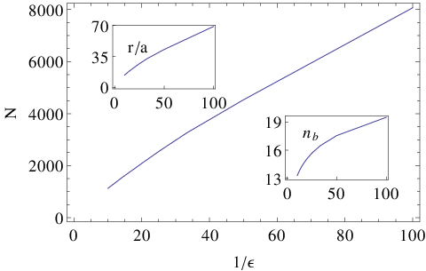
Next, we estimate the necessary number of qubits per site. In §4.1, the constant factors hidden by the big-O notation can easily be restored. Specifically, a sufficient choice is

n_{b}=\left\lceil\log_{2}\left(1+\frac{2a^{d}}{\pi}\left(1+\sqrt{\frac{\mathcal{V}}{\epsilon}}\right)^{2}\sqrt{\langle\phi^{2}\rangle\langle\pi^{2}\rangle}\right)\right\rceil.

(378)

To bound $\langle\phi^{2}\rangle$ and $\langle\pi^{2}\rangle$ , we must estimate the bare quantities $\lambda_{0}$ and $m_{0}^{2}$ and then apply Proposition 3 or 4. In $D=2$ , one finds perturbatively that

	$\displaystyle m_{0}^{2}$	$\displaystyle=$	$\displaystyle m^{2}-\frac{\lambda}{8\pi}\log\left(\frac{64}{m^{2}a^{2}}\right)+\cdots\,,$		(379)
	$\displaystyle\lambda_{0}$	$\displaystyle=$	$\displaystyle\lambda+\frac{3\lambda^{2}}{8\pi m^{2}}+\cdots\,.$		(380)

We must now choose a value of $\lambda$ that is small enough to justify the use of $V^{(2)}$ , but large enough to make classical calculations at high precision difficult. As concrete examples, we consider the values $\frac{\lambda}{2\pi m^{2}}=\frac{1}{3}$ and $\frac{\lambda}{2\pi m^{2}}=\frac{1}{10}$ . The results show that $n_{b}$ is not very sensitive to the choice of $\lambda$ , as discussed below.

For $0.01\leq\epsilon\leq 0.1$ , our choices of $\lambda$ and $ma$ imply that $m_{0}^{2}\geq 0$ , and thus the applicable bound on $\langle\phi^{2}\rangle$ and $\langle\pi^{2}\rangle$ is Proposition 3 throughout the entire adiabatic state preparation. By (378) and Proposition 3, one obtains $n_{b}$ as a function of $\epsilon$ , as shown in the right inset in Fig. 2. Replacing $\frac{\lambda}{2\pi m^{2}}=\frac{1}{3}$ with $\frac{\lambda}{2\pi m^{2}}=\frac{1}{10}$ changes $n_{b}$ from 20 to 19 at $\epsilon=0.01$ and leaves $n_{b}$ unchanged at 13 for $\epsilon=0.1$ . Our estimate of the total number of qubits $N=n_{b}\mathcal{V}$ needed to achieve a given precision $\epsilon$ is plotted in Fig. 2.

Finally, let us comment on the asymptotic scaling of the number of qubits required by our algorithm. As discussed above (see (376)), to restrict discretization errors to order $\epsilon$ we need $ma\sim\sqrt{\epsilon}$ . Furthermore, to obtain good in and out states we need particles to be separated by a distance $r\sim\frac{1}{m}\log(1/\epsilon)$ . Thus, the total number of lattice sites is $\mathcal{V}\sim\left(\frac{r}{a}\right)^{d}=O\left(\epsilon^{-d/2}\log^{d}(1/\epsilon)\right)$ . The number of qubits per site is $n_{b}\sim\log(1/\epsilon)$ . Thus, the total number of qubits is $N=O\left(\epsilon^{-d/2}\log^{d+1}(1/\epsilon)\right)$ . In contrast to the estimate shown in Fig. 2, which relies on perturbative calculations, this asymptotic scaling should hold at both strong and weak coupling. Note that, as mentioned in §3.1, we consider spatially localized wavepackets and the attendant uncertainty in momentum to be physically realistic and not a source of error, although this notion differs from the idealization used to define an $S$ -matrix.

References

[1] D. Hanneke, S. Fogwell, and G. Gabrielse. New measurement of the electron magnetic moment and the fine structure constant. Physical Review Letters, 100:120801, 2008.
[2] Pierre Cladé, Estefania de Mirandes, Malo Cadoret, Saïda Guellati-Khélifa, Catherine Schwob, François Nez, Lucile Julien, and François Biraben. Determination of the fine structure constant based on Bloch oscillations of ultracold atoms in a vertical optical lattice. Physical Review Letters, 96:033001, 2006.
[3] V. Gerginov, K. Calkins, C. E. Tanner, J. J. McFerran, S. Diddams, A. Bartels, and L. Hollberg. Optical frequency measurements of ${}^{2}S_{1/2}-6p^{2}P_{1/2}(D_{1})$ transitions in ${}^{133}Cs$ and their impact on the fine-structure constant. Physical Review A, 73:032504, 2006.
[4] Kenneth Wilson. The renormalization group and critical phenomena. In Nobel Lectures, Physics 1981-1990. World Scientific, 1993. Also available at www.nobelprize.org/nobel_prizes/physics/laureates/1982/wilson-lecture.pdf.
[5] Peter W. Shor. Polynomial-time algorithms for prime factorization and discrete logarithms on a quantum computer. SIAM Journal on Computing, 26:1484–1509, 1997. arXiv:quant-ph/9508027.
[6] A. K. Lenstra and H. W. Lenstra Jr., editors. The development of the number field sieve, volume 1554 of Lecture Notes in Mathematics. Springer-Verlag, 1993.
[7] Stephen Jordan. Quantum algorithm zoo. http://math.nist.gov/quantum/zoo/.
[8] Richard P. Feynman. Simulating physics with computers. International Journal of Theoretical Physics, 21:467–488, 1982.
[9] David Deutsch. Quantum theory, the Church-Turing principle, and the universal quantum computer. Proceedings of the Royal Society of London A, 400:97–117, 1985.
[10] David Deutsch. Quantum computational networks. Proceedings of the Royal Society of London A, 425:73–90, 1989.
[11] Edward Farhi and Sam Gutmann. Quantum computation and decision trees. Physical Review A, 58:915–928, 1998. arXiv:quant-ph/9706062.
[12] Dorit Aharonov, Andris Ambainis, Julia Kempe, and Umesh Vazirani. Quantum walks on graphs. In Proceedings of 33rd ACM Symposium on Theory of Computing (STOC 2001), pages 50–59, 2001. arXiv:quant-ph/0012090.
[13] Alexei Yu Kitaev. Fault-tolerant quantum computation by anyons. Annals of Physics, 303:2–30, 2003. arXiv:quant-ph/9707021.
[14] Edward Farhi, Jeffrey Goldstone, Sam Gutmann, and Michael Sipser. Quantum computation by adiabatic evolution. 2000. arXiv:quant-ph/0001106.
[15] Andrew Chi-Chih Yao. Quantum circuit complexity. In Proceedings of 34th IEEE Symposium on Foundations of Computer Science (FOCS 1993), pages 352–361, 1993.
[16] Andrew M. Childs. Universal computation by quantum walk. Physical Review Letters, 102:180501, 2009. arXiv:0806.1972.
[17] Michael H. Freedman, Alexei Kitaev, and Zhenghan Wang. Simulation of topological field theories by quantum computers. Communications in Mathematical Physics, 227:587–603, 2002. arXiv:quant-ph/0001071.
[18] Michael H. Freedman, Michael Larsen, and Zhenghan Wang. A modular functor which is universal for quantum computation. Communications in Mathematical Physics, 227:605–622, 2002. arXiv:quant-ph/0001108.
[19] Dorit Aharonov, Wim van Dam, Julia Kempe, Zeph Landau, Seth Lloyd, and Oded Regev. Adiabatic quantum computation is equivalent to standard quantum computation. SIAM Journal on Computing, 37:166–194, 2007. arXiv:quant-ph/0405098.
[20] Ethan Bernstein and Umesh Vazirani. Quantum complexity theory. In Proceedings of the 25th ACM Symposium on Theory of Computing (STOC 1993), pages 11–20, 1993.
[21] Christof Zalka. Efficient simulation of quantum systems by quantum computers. Proceedings of the Royal Society of London A, 454:313–322, 1998. arXiv:quant-ph/9603026.
[22] Daniel S. Abrams and Seth Lloyd. Simulation of many-body Fermi systems on a universal quantum computer. Physical Review Letters, 79:2586–2589, 1997.
[23] Stephen Wiesner. Simulations of many-body quantum systems by a quantum computer. arXiv:quant-ph/9603028, 1996.
[24] Seth Lloyd. Universal quantum simulators. Science, 273:1073–1078, 1996.
[25] Tim Byrnes and Yoshihisa Yamamoto. Simulating lattice gauge theories on a quantum computer. Physical Review A, 73:022328, 2006. arXiv:quant-ph/0510027.
[26] Alán Aspuru-Guzik, Anthony D. Dutoi, Peter J. Love, and Martin Head-Gordon. Simulated quantum computation of molecular energies. Science, 309:1704–1707, 2005.
[27] H. P. Büchler, M. Hermele, S. D. Huber, Matthew P. A. Fisher, and P. Zoller. Atomic quantum simulator for lattice gauge theoreis and ring exchange models. Physical Review Letters, 95:040402, 2005.
[28] Erez Zohar and Benni Reznik. Confinement and lattice quantum-electrodynamic electric flux tubes simulated with ultracold atoms. Physical Review Letters, 107:275301, 2011.
[29] Gergely Szirmai, Edina Szirmai, Alejandro Zamora, and Maciej Lewenstein. Gauge fields emerging from time reversal symmetry breaking for spin-5/2 fermions in a honeycomb lattice. Physical Review A, 84:011611(R), 2011.
[30] J. Ignacio Cirac, Paolo Maraner, and Jiannis K. Pachos. Cold atom simulation of interacting relativistic quantum field theories. Physical Review Letters, 105:190403, 2010.
[31] Leonardo Mazza, Alejandro Bermudez, Nathan Goldman, Matteo Rizzi, Miguel Angel Martin-Delgado, and Maciej Lewenstein. An optical-lattice-based quantum simulator for relativistic field theories and topological insulators. New Journal of Physics, 14:015007, 2012.
[32] Eliot Kapit and Erich Mueller. Optical-lattice Hamiltonians for relativistic quantum electrodynamics. Physical Review A, 83:033625, 2011.
[33] A. Bermudez, L. Mazza, M. Rizzi, N. Goldman, M. Lewenstein, and M. A. Martin-Delgado. Wilson fermions and axion electrodynamics in optical lattices. Physical Review Letters, 105:190404, 2010.
[34] Paolo Maraner and Jiannis K. Pachos. Yang-Mills gauge theories from simple fermionic lattice models. Physics Letters A, 373:2542–2545, 2009.
[35] L. Lepori, G. Mussardo, and A. Trombettoni. (3+1) massive Dirac fermions with ultracold atoms in frustrated cubic optical lattices. Europhysics Letters, 92:50003, 2010.
[36] Kenji Maeda, Gordon Baym, and Tetsuo Hatsuda. Simulating dense QCD matter with ultracold atomic boson-fermion mixtures. Physical Review Letters, 103:085301, 2009.
[37] Ákos Rapp, Gergely Zaránd, Carsten Honerkamp, and Walter Hofstetter. Color superfluidity and “baryon” formation in ultracold fermions. Physical Review Letters, 98:160405, 2007.
[38] Hendrik Weimer, Markus Müller, Igor Lesanovsky, Peter Zoller, and Hans Peter Büchler. A Rydberg quantum simulator. Nature Physics, 6:382–388, 2010.
[39] J. Casanova, L. Lamata, I. L. Egusquiza, R. Gerritsma, C. F. Roos, J. J. Garcia-Ripoll, and E. Solano. Quantum simulation of quantum field theories in trapped ions. Physical Review Letters, 107:260501, 2011.
[40] J. Casanova, A. Mezzacapo, L. Lamata, and E. Solano. Quantum simulation of interacting fermion lattice models in trapped ions. Physical Review Letters, 108:190502, 2012. arXiv:1110.3730.
[41] B. Doucot, L. B. Ioffe, and J. Vidal. Discrete non-Abelian gauge theories in two-dimensional lattices and their realizations in Josephson-junction arrays. Physical Review B, 69:214501, 2004. arXiv:cond-mat/0302104.
[42] Maciej Lewenstein, Anna Sanpera, Veronica Ahufinger, Bogdan Damski, Aditi Sen De, and Ujjwal Sen. Ultracold atomic gases in optical lattices: mimicking condensed matter physics and beyond. Advances in Physics, 56:243–379, 2007. arXiv:cond-mat/0606771.
[43] Michael Johanning, Andrés Varón, and Christof Wunderlich. Quantum simulations with cold trapped ions. Journal of Physics B, 42:154009, 2009. arXiv:0905.0118.
[44] Dorit Aharonov and Michael Ben-Or. Fault-tolerant quantum computation with constant error rate. SIAM Journal on Computing, 38:1207–1282, 2008. arXiv:quant-ph/9611025.
[45] Emmanuel Knill, Raymond Laflamme, and Wojciech H. Zurek. Resilient quantum computation. Science, 279:342–345, 1998. arXiv:quant-ph/9702058.
[46] Stephen P. Jordan, Keith S. M. Lee, and John Preskill. Quantum algorithms for quantum field theories. Science, 336:1130–1133, 2012. arXiv:1111.3633.
[47] J. Glimm and A. Jaffe. A $\lambda\phi^{4}$ quantum field theory without cutoffs. I. Physical Review, 176:1945–1961, 1968.
[48] J. Glimm and A. Jaffe. The $\lambda(\phi^{4})_{2}$ quantum field theory without cutoffs: II. the field operators and the approximate vacuum. Annals of Mathematics, 91:362–401, 1970.
[49] J. Glimm and A. Jaffe. The $\lambda(\phi^{4})_{2}$ quantum field theory without cutoffs. III. the physical vacuum. Acta Mathematica, 125:203–267, 1970.
[50] J. Glimm and A. Jaffe. The $\lambda\phi^{4}_{2}$ quantum field theory without cutoffs. IV. perturbations of the Hamiltonian. Journal of Mathematical Physics, 13:1568–1584, 1972.
[51] J. Glimm, A. Jaffe, and T. Spencer. The Wightman axioms and particle structure in the weakly coupled $P(\phi)_{2}$ quantum field model. Annals of Mathematics, 100:585–632, 1974.
[52] J. Glimm and A. Jaffe. Positivity of the $\phi_{3}^{4}$ Hamiltonian. Fortschrift der Physik, 21:327–376, 1973.
[53] Joel S. Feldman and Konrad Osterwalder. The Wightman axioms and mass gap for weakly coupled $(\varphi^{4})_{3}$ quantum field theories. Annals of Physics, 97:80–135, 1976.
[54] K. Osterwalder and R. Sénéor. The scattering matrix is nontrivial for weakly coupled $P(\phi)_{2}$ models. Helvetica Physica Acta, 49:525–536, 1976.
[55] J.-P. Eckmann, H. Epstein, and J. Fröhlich. Asymptotic perturbation expansion for the $S$ matrix and the definition of time ordered functions in relativistic quantum field models. Annales de l’institut Henri Poincaré (A) Physique théorique, 25:1–34, 1976.
[56] F. Constantinescu. Nontriviality of the scattering matrix for weakly coupled $\phi_{3}^{4}$ models. Annals of Physics, 108:37–48, 1977.
[57] J.-P. Eckmann, J. Magnen, and R. Sénéor. Decay properties and Borel summability for the Schwinger functions in $P(\phi)_{2}$ theories. Communications in Mathematical Physics, 39:251–271, 1975.
[58] J. Magnen and R. Sénéor. Phase space cell expansion and Borel summability for the Euclidean $\phi_{3}^{4}$ theory. Communications in Mathematical Physics, 56:237–276, 1977.
[59] J.-P. Eckmann and H. Epstein. Borel summability of the mass and the $S$ -matrix in $\phi^{4}$ models. Communications in Mathematical Physics, 68:245–258, 1979.
[60] Michael Aizenman. Geometric analysis of $\phi^{4}$ fields and Ising models. Parts I and II. Communications in Mathematical Physics, 86:1–48, 1982.
[61] J. Fröhlich. On the triviality of $\lambda\varphi_{d}^{4}$ theories and the approach to the critical point in $d$ 4 dimensions. Nuclear Physics B, 200:281–296, 1982.
[62] David C. Brydges, Jürg Frölich, and Alan D. Sokal. A new proof of the existence and nontriviality of the continuum $\varphi^{4}_{2}$ and $\varphi^{4}_{3}$ quantum field theories. Communications in Mathematical Physics, 91:141–186, 1983.
[63] James Glimm and Arthur Jaffe. $\phi_{2}^{4}$ quantum field model in the single-phase region: Differentiability of the mass and bounds on critical exponents. Physical Review D, 10:536–539, 1974.
[64] F. Guerra, L. Rosen, and B. Simon. Correlation inequalities and the mass gap in $P(\phi)_{2}$ . III. Mass gap for a class of strongly coupled theories with nonzero external field. Communications in Mathematical Physics, 41:19–32, 1975.
[65] O. A. McBryan and J. Rosen. Existence of the critical point in $\phi^{4}$ field theory. Communications in Mathematical Physics, 51:97–105, 1976.
[66] J. C. Le Guillou and Jean Zinn-Justin. Critical exponents for the $n$ -vector model in three dimensions from field theory. Physical Review Letters, 39:95–98, 1977.
[67] M. Lüscher and P. Weisz. Scaling laws and triviality bounds in the lattice $\phi^{4}$ theory. (I). one-component model in the symmetric phase. Nuclear Physics B, 290:25, 1987.
[68] Michael Nielsen and Isaac Chuang. Quantum Computation and Quantum Information. Cambridge, 2000.
[69] E. Fredkin and T. Toffoli. Conservative logic. International Journal of Theoretical Physics, 21:219–253, 1982.
[70] R. Cleve, A. Ekert, C. Macchiavello, and M. Mosca. Quantum algorithms revisited. Proceedings of the Royal Society A, 454:339–354, 1998. arXiv:quant-ph/9708016.
[71] A. Yu Kitaev. Quantum measurements and the Abelian stabilizer problem. 1995. arXiv:quant-ph/9511026.
[72] E. Knill. Approximation by quantum circuits. Technical Report LAUR-95-2225, Los Alamos National Laboratory, 1995. arXiv:quant-ph/9508006.
[73] A. Yu Kitaev, A. H. Shen, and M. N. Vyalyi. Classical and Quantum Computation, volume 47 of Graduate Studies in Mathematics. American Mathematical Society, 2002.
[74] Julia Kempe and Oded Regev. 3-local Hamiltonian is QMA-complete. Quantum Information and Computation, 3:258–264, 2003. arXiv:quant-ph/0302079.
[75] Julia Kempe, Alexei Kitaev, and Oded Regev. The complexity of the local Hamiltonian problem. SIAM Journal on Computing, 35:1070–1097, 2006. arXiv:quant-ph/0406180.
[76] Sabine Jansen, Ruedi Seiler, and Mary-Beth Ruskai. Bounds for the adiabatic approximation with applications to quantum computation. Journal of Mathematical Physics, 48:102111, 2007. arXiv:quant-ph/0603175.
[77] Jeffrey Goldstone. Adiabatic theorem. Recounted in Appendix F of arXiv:0809.2307.
[78] Albert Messiah. Quantum Mechanics. Dover, 1999. Reprint of the two-volume edition published by Wiley, 1961-1962.
[79] Alexei Kitaev and William A. Webb. Wavefunction preparation and resampling using a quantum computer. arXiv:0801.0342, 2008.
[80] Lov Grover and Terry Rudolph. Creating superpositions that correspond to efficiently integrable probability distributions. 2002. arXiv:quant-ph/0208112.
[81] James R. Bunch and John E. Hopcroft. Triangular factorization and inversion by fast matrix multiplication. Mathematics of Computation, 28:231–236, 1974.
[82] Don Coppersmith and Schmuel Winograd. Matrix multiplication via arithmetic progressions. Journal of Symbolic Computation, 9:251–280, 1990.
[83] Virginia Vassilevska Williams. Multiplying matrices faster than Coppersmith-Winograd. In Proceedings of the 44th ACM Symposium on Theory of Computing (STOC 2012), pages 887–898, 2012. Full version: www.cs.berkeley.edu/ $\scriptstyle\mathtt{\sim}$ virgi/matrixmult-f.pdf.
[84] L.N. Lipatov. Divergence of the perturbation theory series and the quasiclassical theory. Sov. Phys. JETP, 45:216–223, 1977.
[85] E. Brézin, J.C. Le Guillou, and J. Zinn-Justin. Perturbation theory at large order. I. the $\phi^{2N}$ interaction. Physical Review D, 15:1544–1557, 1977.
[86] M. Suzuki. Fractal decomposition of exponential operators with applications to many-body theories and Monte Carlo simulations. Physics Letters A, 146:319–323, 1990.
[87] D.W. Berry, G. Ahokas, R. Cleve, and B. C. Sanders. Efficient quantum algorithms for simulating sparse Hamiltonians. Communications in Mathematical Physics, 270:359–371, 2007. arXiv:quant-ph/0508139.
[88] Masuo Suzuki. General decomposition theory of ordered exponentials. Proceedings of the Japan Academy Ser. B, 69:161–166, 1993.
[89] Nathan Wiebe, Dominic Berry, Peter Høyer, and Barry C. Sanders. Higher order decompositions of ordered operator exponentials. Journal of Physics A: Mathematical and Theoretical, 43:065203, 2010.
[90] K. Symanzik. Cutoff dependence in $\phi^{4}_{4}$ theory. In G. ’t Hooft, editor, Cargése Lectures 1979, page 313, New York, 1980. Plenum.
[91] K. Symanzik. Continuum limit and improved action in lattice theories. 1. principles and $\phi^{4}$ theory. Nuclear Physics B, 226:187, 1983.
[92] K. Symanzik. Continuum limit and improved action in lattice theories. 2. $O(N)$ nonlinear sigma model in perturbation theory. Nuclear Physics B, 205:205, 1983.
[93] Christopher Arzt. Reduced effective Lagrangians. Physics Letters B, 342:189–195, 1995.
[94] Howard Georgi. On-shell effective field theory. Nuclear Physics B, 361:339–350, 1991.
[95] L. Eulero. Methodus generalis summandi progressiones. Commentarii academiae scientiarum imperialis Petropolitanae, 6:68, 1732. Reprinted in his Opera Omnia, ser. 1, vol. 14, 42.
[96] S. D. Poisson. Mémoire sur le calcul numérique des intégrales définies. Mémoires de l’Académie Royale des Sciences de l’Institut de France ser. 2, 6:571, 1823.
[97] Daniel Gottesman. An introduction to quantum error correction and fault-tolerant quantum computation. In Quantum Information Science and its Contributions to Mathematics, Proceedings of Symposia in Applied Mathematics 68, pages 13–58. American Mathematical Society, 2010. arXiv:0904.2557.

Quantum Computation of Scattering in Scalar Quantum Field Theories

Abstract

1 Introduction

2 Background

2.1 Quantum Field Theory

2.1.1 Lattice ϕ4\phi^{4} Theory

2.1.2 Continuum Limit

2.1.3 Phase Transitions

2.2 Quantum Computing

2.2.1 Quantum Fourier Transform

2.2.2 Reversible Circuits and Phase Kickback

2.2.3 Phase Estimation

2.2.4 Simulating Hamiltonian Time Evolution

2.2.5 Adiabatic State Preparation

3 Quantum Algorithm

3.1 Description and Discussion

3.2 Efficiency

4 Analysis of Algorithm

4.1 Representation by Qubits

Proposition 1.

Proof.

Proposition 2.

Proof.

Proposition 3.

Proof.

Proposition 4.

Proof.

4.2 Adiabatic Preparation of Interacting Wavepackets

4.2.1 Weak Coupling

4.2.2 Strong Coupling

4.3 Suzuki-Trotter Formulae for Large Lattices

Theorem 1.

4.4 Measurement of Occupation Numbers

4.5 Detection of Bound States

4.6 Localized Creation Operators

5 Some Field-Theoretical Aspects

5.1 Mass Renormalization

5.1.1 The Discretized Theory

5.1.2 The Physical Mass

5.2 Effective Field Theory

5.3 Effects of Non-zero Lattice Spacing

5.3.1 The General Effective Theory

5.3.2 Matching

Operators induced purely by Discretization

Operators induced by Quantum Effects

Lorentz-Violating Operators induced by Quantum Effects

5.3.3 Strong Coupling

5.4 Effects of Finite Volume on EFT

5.5 Effect of Finite Volume on State Preparation

6 Conclusions

Appendices

A. Notation

B. Loop Integrals for Mass Renormalization

C. Loop Integrals for Matching

D. Loop Sums for Matching

E. Integrals for Effective Potential

F. Minimal Qubit Requirement

References

Quantum Computation of Scattering
in Scalar Quantum Field Theories

2.1.1 Lattice $\phi^{4}$ Theory