Approximate Bayesian computation and
Bayes linear analysis: Towards high-dimensional ABC

As in Section 1, suppose that $s=s(y)=(s_{1},...,s_{d})^{\top}$ is some vector of summary statistics based on data $y$, and that $\theta=(\theta_{1},...,\theta_{p})^{\top}$ denotes parameter unknowns that we wish to learn about. One view of Bayes linear analysis (e.g. [Goldstein and Wooff 2007]) is that it aims to construct an optimal linear estimator of $\theta$ under squared error loss. That is, an estimator of the form $a+Bs$, for a $p$-dimensional vector, $a$, and a $p\times d$ matrix, $B$, minimising

The optimal linear estimator is given by

where expectations and covariances on the right hand side are with respect to the joint prior distribution of $s$ and $\theta$ i.e. $p(s|\theta)p(\theta)$. The estimator, $E_{s}(\theta)$, is referred to as the adjusted expectation of $\theta$ given $s$. If the posterior mean is a linear function of $s$ then the adjusted expectation and posterior mean coincide. Note that obtaining the best linear estimator of $\theta$ does not require specification of a full prior or likelihood – only first and second order moments of $(\theta,s)$ are needed. From a subjective Bayesian perspective, the need to make only a limited number of judgements concerning prior moments is a key advantage of the Bayes linear approach. There are various interpretations of Bayes linear methods – see ?), for further discussion. In the ABC context, a full probability model is typically available. As such, we will consider Bayes linear analysis from a conventional Bayesian point of view as a computational approximation to a full Bayesian analysis.

The adjusted variance of $\theta$ given $s$, $\mbox{Var}_{s}(\theta)=E[(\theta-E_{s}(\theta))^{\top}(\theta-E_{s}(\theta)]$, can be shown to be

Furthermore, the inequality $\mbox{Var}_{s}(\theta)\geq E[\mbox{Var}(\theta|s)]$ holds, where $A\geq C$ means that $A-C$ is non-negative definite, and the outer expectation on the right hand side is with respect to the prior distribution for $s$, $p(s)$. This inequality indicates that $\mbox{Var}_{s}(\theta)$ is a generally conservative upper bound on posterior variance, although it should be noted that $\mbox{Var}_{s}(\theta)$ does not depend on $s$, whereas $\mbox{Var}(\theta|s)$ is fully conditional on the observed $s$. If the posterior mean is a linear function of $s$, then $\mbox{Var}_{s}(\theta)=E[\mbox{Var}(\theta|s)]$

It is relatively straightforward to link the regression-adjustment approach of ?) with a Bayes linear analysis. However, note that ?) do not consider the model (2) as holding globally, but instead assume that it holds locally around the observed summary statistics, $s$. We discuss this point further below, but for the moment we assume that the unweighted linear model (2) holds globally, after an appropriate choice of the summary statistics, $s$.

The ordinary least squares estimate of $\beta$ under the linear model (2) is $\hat{\beta}=\hat{\Sigma}(s)^{-1}\hat{\Sigma}(s,\theta)$, where $\hat{\Sigma}(s)$ is the sample covariance of $s^{1},...,s^{n}$ and $\hat{\Sigma}(s,\theta)$ is the sample cross covariance of the pairs $(s^{i},\theta^{i})$, $i=1,...,n$. For large $n$ (where $n$ is a quantity under direct user control in an ABC analysis), $\hat{\beta}$ is approximately $\beta=\mbox{Var}(s)^{-1}\mbox{Cov}(s,\theta)$, where $\mbox{Var}(s)$ and $\mbox{Cov}(s,\theta)$ are the corresponding population versions of $\hat{\Sigma}(s)$ and $\hat{\Sigma}(s,\theta)$. Let $i$ be fixed and consider the sequence of random variables $\theta^{i,a}=\theta^{i}-\hat{\beta}^{\top}(s^{i}-s)$ as $n$ tends to infinity. Note that $\hat{\beta}$ is a function of $(\theta^{j},s^{j})$ for $j=1,...,n$ here. By Slutsky’s theorem, if $\hat{\beta}$ is consistent for $\beta$ then $\theta^{i,a}$ will converge in probability and in distribution to $\theta^{i}-\beta^{\top}(s^{i}-s)$ as $n\rightarrow\infty$. Then we can write

where the interchange of limits in the first line can be justified by applying the Skorohod representation theorem and then the dominated convergence theorem.

By a similar argument

Hence, the covariance matrix of the regression-adjusted $\theta^{i,a}$ approximates the Bayes linear adjusted variance for large $n$.

These results demonstrate that the first and second moments of the regression-adjusted samples $\theta^{i,a}$, $i=1,...,n$ in the linear method of ?) have a useful interpretation, regardless of whether the linear assumptions of the regression model (2) hold globally, as a Monte Carlo approximation to a Bayes linear analysis. This connection with Bayes linear analysis is not surprising when one considers that a Monte Carlo approximation to (4) based on draws from the prior is just a least squares criterion for regression of $\theta$ on $s$. Usefully for our present purposes, the Bayes linear interpretation may be helpful for motivating an exploratory use of regression adjustment ABC, even in problems of high dimension. In high-dimensional problems, an anonymous referee has suggested it might also be useful to consider more sophisticated shrinkage estimates of covariance matrices in implementing the Bayes linear approach. The connection between Bayes linear methods and regression-adjustment ABC continues to hold if kernel weighting is reincorporated into the regression model (2). Now consider the model (1) in general and a Bayes linear analysis using first and second order moments of $(\theta,s^{*})|s$ with Bayes linear updating by the information $s=s^{*}$. This then corresponds to the kernel weighted version of the procedure of ?).

A recent extension of regression-adjustment ABC is the nonlinear, heteroscedastic method of ?) which replaces (2) with

where $\mu(s^{i})=E(\theta|s=s^{i})$ is a mean function, $\sigma(s^{i})$ is a diagonal matrix with diagonal entries equal to the square roots of the diagonal entries of $\mbox{Var}(\theta|s=s^{i})$, and the $\varepsilon^{i}$ are i.i.d. zero mean random vectors with $\mbox{Var}(\varepsilon^{i})=I$. It is possible also to take $\sigma(s)$ to be some matrix square root of $\mbox{Var}(\theta|s=s^{i})$ where all elements are functions of $s$. If (5) holds, then the adjustment

is a draw from $p(\theta|s)$. The heteroscedastic adjustment approach does seem to be outside the Bayes linear framework. However, a nonlinear mean model for $\mu(s)$ with a constant model for $\sigma(s)$ can be reconciled with the Bayes linear approach by considering an appropriate basis expansion involving functions of $s$. ?) gives some theoretical support for more complex regression adjustments through an analysis of a certain quadratic regression adjustment and suggests that transformations of $\theta$ can be used to deal with heteroscedasticity. In this case, the Bayes linear interpretation would be more broadly applicable in regression-adjustment ABC. Another recent regression adjustment approach is that of ?), which is based on fitting a flexible mixture model to the joint samples.

An interesting recent related development is the semi-automatic method of choosing summary statistics of ?). They consider an initial provisional set of statistics and then use linear regression to construct a summary statistic for each parameter, based on samples from the prior or some truncated version of it. Their approach can be seen as a use of Bayes linear estimates as summary statistics for an ABC analysis. There are several other innovative aspects of their paper but their approach to summary statistic construction provides another strong link with Bayes linear ideas.

We first construct a toy example where the likelihood can be evaluated and where a gold standard answer is available for comparison. While ABC methods are not needed for the analysis of this model, it is instructive for understanding the properties of our methods. We consider a $p$-dimensional Gaussian mixture model with $2^{p}$ mixture components. The likelihood for this model is given by

where $\phi_{p}(x|a,B)$ denotes the $p$-dimensional Gaussian density function with mean $a$ and covariance $B$ evaluated at $x$, $\omega\in[0,1]$ is a mixture weight, $\mu(b,\theta)^{\top}=((1-2b_{1})\theta_{1},\ldots,(1-2b_{p})\theta_{p})$, $b=(b_{1},\ldots,b_{p})$ with $b_{i}\in\{0,1\}$ and $\Sigma=[\Sigma_{ij}]$ is such that $\Sigma_{ii}=1$ and $\Sigma_{ij}=\rho$ for $i\neq j$. Under this setting, the marginal distribution for $s_{i}$ is given by the two-component mixture

The combination of the $p$ two-mixture-component marginal distributions forms the $2^{p}$ mixture components for the $p$-dimensional model. Given $\theta$, data generation under this model proceeds by independently generating each component of $b$ to be $0$ or $1$ with probabilities $\omega$ and $1-\omega$ respectively, and then drawing $s|\theta,b\sim\phi_{p}(\mu(b,\theta),\Sigma)$.

For the following analysis we specify $s=(5,5,\ldots,5)$, $\omega=0.3$ and $\rho=0.7$, and restrict the posterior to have finite support on $[-20,40]^{p}$, over which we have a uniform prior for $\theta$. Computations are performed using 1 million simulations from $p(s|\theta)p(\theta)$, using a uniform kernel $K_{\epsilon}(\|u\|)$, where $\|\cdot\|$ denotes Euclidean distance, and where $\epsilon$ is chosen to select the 10,000 simulations closest to $s$. We contrast results obtained using standard rejection sampling, rejection sampling followed by the regression-adjustment of ?), and both of these after applying our marginal-adjustment strategy. All inferences were performed using the R package abc [Csilléry, François, and Blum 2011].

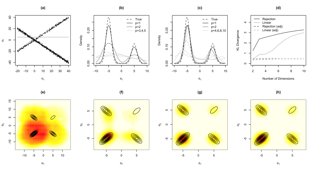
Figure 1(a) illustrates the relationship between $\theta_{1}$ and $s_{1}$ (all margins are identical), with around 70% of summary statistics located in the line with negative slope. The observed summary statistic is indicated by the horizontal line, the marginal posterior distribution for $\theta_{1}$ defined by the implied density of summary statistics on this line. Figure 1(b) shows density estimates of $\theta_{1}|s$ using rejection sampling for $p=1,2,\ldots,5$ model dimensions. The univariate true marginal distribution is indicated by the dashed line. As model dimension increases, the quality of the approximation to the true marginal distribution deteriorates rapidly. This is due to the curse of dimensionality in ABC (e.g. [Blum 2010]) in which the restrictions on $s_{1}$ for a fixed number of accepted samples (in this case 10,000) decrease within the comparison $\|s-s^{*}\|$ as $p$ increases. Of course one could increase the number of simulations as the dimension increases, but assuming a fixed computational budget returning a fixed number of samples provides one perspective on the curse of dimensionality here. Beyond $p=2$ dimensions, these density estimates are exceptionally poor. The same information is illustrated in Figure 1(c) after applying the linear regression-adjustment of ?) to the samples obtained by rejection sampling in Figure 1(b). Clearly the regression-adjustment is beneficial in providing improved marginal density estimates. However, the quality of the approximation still deteriorates quickly as $p$ increases, albeit more slowly than for rejection sampling alone.

Figures 1(e) and (f) show the two dimensional density estimates of $(\theta_{1},\theta_{2})|s$ for the $p=3$ dimensional model, respectively using rejection sampling, and rejection sampling followed by the linear regression-adjustment. The superimposed contours correspond to those of the true bivariate marginal distribution. The improvement to the density estimate following the regression-adjustment is clear, however even here, the component modes appear to be slightly misplaced, and there is some blurring of density with neighbouring components.

Figures 1(g) and (h) correspond to the densities in Figures 1(e) and (f) after the implementation of our marginal adjustment strategy. Here, each margin of the distributions is adjusted to be that of the appropriate univariate marginal density estimate in a $p=1$ dimensional analysis. E.g. the margins for $\theta_{1}$ are adjusted to be exactly the ($p=1$) density estimates in Figures 1(b) and (c). In both plots (g and h) there is a clear improvement in the bivariate density estimate: the locations of the mixture components are in the correct places, and on the correct scales. Some of the accuracy of the dependence structure is less well captured under just rejection sampling, however (Figure 1(g)). Here, the correlation structure of each Gaussian component seems to be poorly estimated, compared to that obtained under the regression-adjustment transformed samples. The message here is clear: any marginal adjustment strategy cannot recover from a poorly estimated dependence structure. The regression adjusted density in Figure 1(f) more accurately captures the correlation structure of the true density, and this improved dependence structure is carried over to the final density estimate in Figure 1(h).

Finally, Figure 1(d) examines the quality of the ABC approximation to the true density, $p(\theta|s)$. Plotted is the Kullback-Leibler divergence, $\int p(\theta)\log\left[p(\theta)/q(\theta)\right]d\theta$, between the densities of the first two dimensions of each distribution as a function of model dimension (where $p(\theta)=p(\theta_{1},\theta_{2}|s)$ is the true density, and $q(\theta)=q(\theta_{1},\theta_{2}|s)$ is a kernel density estimate of the ABC approximation). The divergence is computed by Monte Carlo integration using 2,000 draws from the true density. We compare only the first two dimensions of the $p$-dimensional posteriors to maintain computational accuracy, noting that all pairwise marginal distributions of the full posterior are identical in this analysis (similarly for all higher-dimensional marginals) .

Figure 1(d) largely supports our previous conclusions. The performance of the rejection sampler and the rejection sampler with regression-adjustment deteriorates rapidly as the number of model dimensions (i.e. summary statistics) increases, although the latter performs better in this regard. There is a clear improvement to both of these approaches gained though our marginal adjustment strategy, with the modified regression-adjustment samples performing marginally better (for this example) where the original regression-adjustment provides better estimates of the multivariate dependence structure in lower dimensions.

After around $p=5$ dimensions there is little difference between the two marginally adjusted posteriors, and the divergence levels off to a constant value independent of model dimension. This is result of the ABC setup for this analysis. Beyond around $p=5$ dimensions, there is little difference between the rejection sampling and regression-adjusted posteriors (e.g. Figures 1(e) and (f)), both largely representing near-uniform distributions over $\theta$. Hence, our marginal adjustment strategy is only able to make the same degree of improvements, regardless of model dimension. The correlation dependence structure is also lost beyond this point, so the expected benefit of the regression-adjustment prior to marginal regression adjustment, is nullified. Using a lower initial threshold, $\epsilon$ (computation permitting), would allow a more accurate initial ABC analysis, and hence more discrimination between the rejection sampling and regression-adjustment approaches.

We now consider the medium resolution version of the heather incidence data analysed by ?), which is available in the R package spatstat [Baddeley and Turner 2005]. Figure 2 illustrates the data, consisting of a $256\times 512$ grid of zeros and ones, with each binary variable representing presence (1) or absence (0) of heather at a particular spatial location.

?) used excursion sets of Gaussian random fields to model a low resolution version of these data. Without loss of generality, we assume that the data are observed on an integer lattice.

Let $\{Y(t);t\in{\mathbb{R}}^{2}\}$ be a stationary Gaussian random field with mean zero and covariance function

where $s,t\in{\mathbb{R}}^{2}$ and where $A$ is a symmetric positive definite matrix. Hence $R(s,t)$ corresponds to the Gaussian covariance function model with elliptical anisotropy. The $u$-level excursion set of $Y(t)$ is defined as $E_{u}(Y)=\{t\in{\mathbb{R}}^{2}:Y(t)\geq u\}$, so that $E_{u}(Y)$ is obtained by “thresholding” $Y(t)$ at level $u\in{\mathbb{R}}$. For background on Gaussian random fields and geometric properties of their excursion sets see e.g. ?).

We model the heather data as binary random variables which are indicators for inclusion in an excursion set on an integer lattice. The data are denoted $B=\{B(i,j):i=0,...,255,j=0,...,511\}$ where $B(i,j)=I((i,j)\in E_{u}(Y))$ and where $I(\cdot)$ denotes the indicator function. The distribution of $B$ clearly depends on $u$ and $A$. We write the $(i,j)$th element of $A$ as $A_{ij}$. Since $A$ is symmetric, $A_{12}=A_{21}$. We parametrize the distribution of $B$ through $\theta=(\theta_{1},\theta_{2},\theta_{3},\theta_{4})$ where $\theta_{1}=u$, $\theta_{2}=\log A_{11}$, $\theta_{3}=\log A_{22}$ and $\theta_{4}=\mbox{logit}[(A_{12}/\sqrt{A_{11}A_{22}}+1)/2]$. We adopt the independent prior distributions $\theta_{1}\sim N(0,0.5^{2})$, $\theta_{2},\theta_{3}\sim N(-4,0.5^{2})$ and $\theta_{4}\sim N(0,0.5^{2})$. The priors here are fairly noninformative. For example, note that the expected fraction of ones in the image is $1-\Phi(\theta_{1})$. Hence if we were to use a normal prior for $\theta_{1}$ with very large variance, this would give roughly prior probability 0.5 to having all zeros and probability 0.5 to have all ones. This is an unreasonable and highly informative prior. Our prior is fairly noninformative for the expected fraction of ones. Similarly our prior on $\theta_{2}$ and $\theta_{3}$ assigns roughly 95% prior probability for correlation in the east-west and north-south directions at lag 10 respectively being between zero and 0.5. For $\theta_{4}$, there is approximately 95% prior probability that $A_{12}/\sqrt{A_{11}A_{22}}$ (a kind of correlation parameter describing the degree of anistropy for the covariance function) lies between $-0.5$ and $0.5$. The results reported below are not sensitive to changes in these priors within reason, but as mentioned highly diffuse priors with large variances are not appropriate. Simulation of Gaussian random fields is achieved with the RandomFields package in R [Schlather 2011], using the circulant embedding algorithm of ?) and ?).

For summary statistics, denote by $n_{11}(v)$ for $v\in{\mathbb{R}}^{2}$ the number of pairs of variables in $B$, separated by displacement $v$, which are both 1. Similarly denote by $n_{00}(v)$ the number of such pairs which are both zero, and by $n_{01}(v)$ the number of pairs where precisely one of the pair is 1 (the order does not matter). In terms of estimating each marginal distribution $\theta_{1}|s(1),\ldots,\theta_{4}|s(4)$, we specify

as the summary statistics for each parameter, where $v_{1}=(0,1)$, $v_{2}=(1,0)$, $v_{3}=(1,1)$ and $v_{4}=(1,-1)$.

For the joint posterior regression-adjustment, we used the heteroscedastic, non-linear regression (5) [Blum and François 2010], using the uniform kernel, $K_{\epsilon}(\|\cdot\|)$, with scale parameter set to give non-zero weight to all $2,000$ samples $(\theta^{i},s^{i})\sim p(s|\theta)p(\theta)$, and where $\|\cdot\|$ represents scaled Euclidean distance. The individual marginal distributions were estimated in the same manner, but with the kernel scale parameter specified to select the 1,000 simulations closest to each $s(j)$. All analyses were again performed using the R package abc [Csilléry, François, and Blum 2011] with the default settings for the heteroscedastic nonlinear method.

Figure 3 shows estimated marginal posterior distributions for the components of $\theta$ obtained by the joint regression-adjustment (dotted lines), and the same margins following our marginal adjustment strategy (solid lines). The estimates for the spatial dependence parameters $\theta_{2}$ and $\theta_{3}$ are poor for the joint regression approach – the individually estimated marginals are estimated very accurately, which can be verified by a rejection based analysis with a much larger number of samples (results not shown). Clearly if we use samples from the approximate joint posterior distribution from the global regression for predictive inference or other purposes, the fact that the unadjusted marginals are centred in the wrong place can lead to unacceptable performance of the approximation.

It is interesting to understand why the global regression approach fails here. Some insight can be gained from Figure 4, which illustrates (prior predictive) scatter plots of $\theta_{2}$ versus $n_{01}(v_{1})$ and $\theta_{3}$ versus $n_{01}(v_{2})$. The summary statistics $n_{01}(v_{1})$ and $n_{01}(v_{2})$ are those which are most informative about $\theta_{2}$ and $\theta_{3}$ respectively. If we consider regression of each of these parameters on the summary statistics, the graphs show that not only the mean and variance, but also higher order properties, such as skewness of the response, appear to change as a function of the summary statistics. As such, the heteroscedastic regression-adjustment based on flexible estimation of the mean and variance does not work well here. Making the regression local for each marginal helps to overcome this problem.

We now examine methods for the analysis of computer models, where we aim to account for uncertainty in high-dimensional forcing functions, assessment of model discrepancy and data rounding. An approximate treatment of this problem is interesting from a model assessment point of view, where we want to judge whether the deficiencies of a computer model are such that the model may be unfit for some purpose.

A computer model can be regarded as a function $y=f(\eta)$ where $\eta$ are model inputs and $y$ is a vector of outputs. In modelling some particular physical system, observed data, $d$, is typically available that corresponds to some subset of the model outputs, $y$. The model inputs, $\eta$, can be of different types. Here we only make the distinction between model parameters, $\theta^{*}$, and forcing function inputs, $\omega$, so that $\eta=(\omega,\theta^{*})$. Commonly, measurements of the forcing function inputs are available, and uncertainty in these inputs (due to e.g. sampling and measurement errors) will be ignored in any analysis due to the high-dimensionality involved. An uncertainty analysis (involving an order of magnitude assessment of output uncertainty due to forcing function uncertainty) will often be performed, rather than attempting to include forcing function uncertainty directly in a calibration exercise (see, for example, [Goldstein, Seheult, and Vernon 2010], for an example of this in the context of a hydrological model). See e.g. ?), ?), ?) and ?) for further discussion of different aspects of computer models.

We now assume that $y=f(\eta)$ corresponds to a prediction of the observed data $d$ in the model

where $e$ denotes measurement error and other sources of error independent in time, and $g$ is a correlated error term representing external model discrepancy (see [Goldstein, Seheult, and Vernon 2010] for a discussion of the differences between internal and external model discrepancies). We directly investigate forcing function uncertainty, through the term $f(\eta)$, using ABC. In the analysis of the model (7), we also consider data rounding effects, so that simulations produced from (7) are rounded according to the precision of the data that was collected. Handling such rounding effects is very simple in the ABC framework.

As a computer model, we consider the Australian Water Balance Model (AWBM) ([Boughton 2004]), a rainfall-runoff model widely used in Australia for applications such as estimating catchment water yield or designing flood management systems.

As shown in Figure 5, the model consists of three surface stores, with depths $c_{1},c_{2},c_{3}$ and fractional areas $a_{1},a_{2},a_{3}$ with $\sum_{k}a_{k}=1$, and a base store. Model forcing inputs are precipitation and evapotranspiration time series, from which a predicted streamflow is produced. At each time step in the model, precipitation is added to the system and evapotranspiration subtracted, with the net input split between the surface stores in proportion to the fractional areas. Any excess above the surface store depths is then split between surface runoff and flow into the base store according to the baseflow index $0<BFI<1$. Water from the base store is discharged into the stream at a rate determined by the recession constant $0<K<1$, and the total discharge (streamflow) is then determined as the sum of the surface runoff and the baseflow. Following ?), we fix $BFI=0.4$, although in some applications it may be beneficial to allow this parameter to vary. The model parameters are therefore $\theta^{*}=(c_{1},c_{2},c_{3},a_{1},a_{2},K)$, as well as the high-dimensional evapotranspiration and precipitation forcing inputs, $\omega$. In hydrological applications there is often great uncertainty about the precipitation inputs in particular, due to measurement and sampling errors. Here we assume that evapotranspiration is fixed (known), and we use $\omega_{obs}$ to denote the series of observed precipitation values only. In running the computer model, we initialize with all stores empty and discard the first 500 days of the simulation to discount the effect of the assumed initial conditions. Our data consist of a sequence of 5500 consecutive daily streamflow values from a station at Black River at Bruce Highway in Queensland, Australia. The catchment covers an area of 260km² with a mean annual rainfall of 1195mm.

To complete the determination of the computer model (7), we specify the model priors. Writing $\eta=(\omega,\theta^{*})$, we describe the uncertainty on the true forcing inputs, $\omega=(\omega_{1},\ldots,\omega_{T})$, as $\omega_{t}=\delta_{t}\omega_{obs,t}$, where the random multiplicative terms have prior $\log\delta_{t}\sim N(-\sigma_{\delta}^{2}/2,\sigma_{\delta}^{2})$ for $t=1,...,T$. We set $\sigma_{\delta}\sim U(0,0.1)$, and note that $E(\delta_{t})=1$ a priori. For the external model discrepancy parameters, $g=(g_{1},\ldots,g_{T})^{\top}$, we specify $g\sim N(0,\Sigma_{g})$ where $\Sigma_{g}=[\Sigma_{g,ij}]$ is such that $\Sigma_{g,ij}=\sigma_{g}^{2}\exp(-\rho|i-j|)$ , $\sigma_{g}\sim U(0,0.1)$ and $\rho\sim U(0.1,1)$. Independent model errors, $e=(e_{1},\ldots,e_{T})^{\top}$, are assumed to be $e_{t}\sim N(0,\sigma_{e}^{2})$, for $t=1,...,T$ where $\sigma_{e}\sim U[0,2]$. AWBM parameter priors are specified as $c_{1}\sim U(0,500)$, $c_{2}-c_{1}\sim U(0,1000)$, $c_{3}-c_{2}\sim U(0,1000)$, $[\log(a_{1}/a_{3}),\log(a_{2}/a_{3})]^{\top}\sim N(0,0.5^{2}I)$ and $K\sim 0.271\times\mbox{Beta}(5.19,4.17)+(1-0.271)\times\mbox{Beta}(255,9.6)$, where the latter is a mixture of beta distributions. See ?) for discussion of the background knowledge leading to this prior choice.

If we treat the forcing inputs, $\omega$, as nuisance parameters, our parameter of interest is $\theta=(\theta^{*\top},\gamma^{\top})^{\top}$, the set of AWBM model parameters, and $\gamma=(\sigma_{e},\sigma_{g},\sigma_{q},\rho)^{\top}$, those parameters specifying distributions of the stochastic terms in (7). The ABC approach provides a convenient way of integrating out the high-dimensional nuisance parameter, $\omega$, while dealing with complications such as rounding in the recorded data (the streamflow data are rounded to the nearest 0.01mm). This would be very challenging using conventional Bayesian computational approaches.

To define summary statistics, denote $\hat{\theta}^{*}$ as the posterior mode estimate of $\theta^{*}$ in a model where we assume no input uncertainty, $\omega=\omega_{obs}$, and where we log-transform both the data and model output. Also denote by $s_{\gamma}=[\psi(0),\psi(1),\psi(2),\zeta(1),\zeta(2),\zeta(3)]^{\top}$, where $\psi(j)$ is the lag $j$ autocovariance of the least squares residuals $d-f(\hat{\eta})$, and $\zeta(j)$ is the lag $j$ autocovariance of $(d-f(\hat{\eta}))^{2}$ with $\hat{\eta}=(\omega_{obs},\hat{\theta}^{*})$. In the notation of Section 3, for summary statistics for $\theta_{j}$, $j=1,...,6$ (i.e. the components of $\theta^{*}$; the AWBM parameters) we use the statistic $s(j)=\hat{\theta}^{*}_{j}$ and for $\theta_{j}$, $j=7,...,10$ (i.e. the components of $\gamma$) we use the statistic $s(j)=s_{\gamma}$. In effect, the summary statistics for $\theta^{*}$ consist of point estimates for the AWBM parameters under the assumption of no error in the forcing inputs, $\omega$, and statistics for the model error parameters, $\gamma$, are intuitively based on autocovariances of residuals and squared residuals. Optimisation of $\hat{\theta}^{*}$ is not trivial, as the objective function may have multiple modes. To provide some degree of robustness, we select the best of ten Nelder-Mead simplex optimisations ([Nelder and Mead 1965]) using starting values simulated from the prior.

Estimated marginal posterior distributions for the parameters are shown in Figure 6.

For the joint-posterior analysis, we implemented the non-linear, heteroscedastic, regression-adjustment of ?) using the uniform kernel, $K_{\epsilon}(\|\cdot\|)$, with scale parameter set to give non-zero weight to all 2,000 samples $(\theta^{i},s^{i})\sim p(s|\theta)p(\theta)$. For the individually estimated margins, the scale parameter was specified to select the 500 simulations closet to each $s(j)$. The discrepancy between estimates for the parameters $c_{1}$, $K$ and $\sigma_{e}$ is particularly striking. To understand why the joint posterior regression-adjustment fails, Figure 7 shows prior predictive scatterplots of these parameters, each against their most informative summary statistic. Similar to the heather incidence example, the distribution of the response evidently changes as a function of the covariates in more complicated ways than just through the first two moments. This is the root cause of the difficulties with the joint regression-adjustment approach. Clearly, the fact that the unadjusted marginals are centred in the wrong place is unacceptable for inferential purposes.

It is difficult here to do cross-validation or the usual predictive checks since this would involve simulating from the posterior distribution for the high-dimensional nuisance parameter, $\omega$, which is precisely what we have used ABC methods to avoid doing. Instead, we examine the raw output of the AWBM model based on the available posterior, assuming no input uncertainty and model discrepancy. As a measure of model fit, we compute the median absolute error over time compared to the observed streamflow, on a log scale i.e. $\mbox{median}\left[\mbox{abs}(\log(d+1))-\log(f(\hat{\eta})+1))\right]$. The boxplots in Figure 6 (bottom right panel) show the distribution of this within sample measure of fit across the two methods. The highly inappropriate posterior estimate of the unadjusted method leads to a worse model fit. Although we have ignored model discrepancy and input uncertainty, we believe these results provide some independent verification of the unsuitability of the unadjusted posterior.

A tentative conclusion from the above analysis is that input uncertainty (through the multiplicative perturbation on the precipitation inputs, $\omega$, controlled through the term $\sigma_{\delta}$) may explain more of the model misfit than the external model discrepancy term ($g$). As such, the AWBM may be an acceptable model for the data given the inherent uncertainty in the forcing inputs.

SAS is supported by the Australian Research Council through the Discovery Project Scheme (DP1092805). The Authors thank M. G. B. Blum for useful discussion on regression-adjustment methods. DJN gratefully acknowledges the support and contributions of the Singapore-Delft Water Alliance (SDWA). The research presented in this work was carried out as part of the SDWAs multi-reservoir research programme (R-264-001-001-272).

References

- Adler and Taylor 2007 Adler, R. J. and J. E. Taylor (2007). Random fields and geometry. Springer Monographs in Mathematics. Springer.
- Baddeley and Turner 2005 Baddeley, A. and R. Turner (2005). Spatstat: Data analysis of spatial point patterns in R. Journal of Statistical Software 12, 1–42.
- Bates and Campbell 2001 Bates, B. and E. Campbell (2001). A Markov chain Monte Carlo scheme for parameter estimation and inference in conceptual rainfall-runoff modeling. Water Resources Research 37, 937–947.
- Beaumont 2010 Beaumont, M. A. (2010). Approximate Bayesian computation in evolution and ecology. Annu. Rev. Ecol. Evol. Syst. 41, 379–406.
- Beaumont, Robert, Marin, and Corunet 2009 Beaumont, M. A., C. P. Robert, J.-M. Marin, and J. M. Corunet (2009). Adaptivity for abc algorithms: The ABC-PMC scheme. Biometrika 96, 983–990.
- Beaumont, Zhang, and Balding 2002 Beaumont, M. A., W. Zhang, and D. J. Balding (2002). Approximate Bayesian computation in population genetics. Genetics 162, 2025–2035.
- Bertorelle, Benazzo, and Mona 2010 Bertorelle, G., A. Benazzo, and S. Mona (2010). ABC as a flexible framework to estimate demography over space and time: Some cons, many pros. Molecular Ecology 19, 2609–2625.
- Blum 2010 Blum, M. G. B. (2010). Approximate Bayesian computation: A non-parametric perspective. Journal of the American Statistical Association 105, 1178–1187.
- Blum and François 2010 Blum, M. G. B. and O. François (2010). Non-linear regression models for approximate Bayesian computation. Statistics and Computing 20, 63–75.
- Blum, Nunes, and Sisson 2012 Blum, M. G. B., M. A. Nunes, and S. A. Sisson (2012). A comparative review of dimension reduction methods in approximate Bayesian computation. Statistical Science, in press.
- Bortot, Coles, and Sisson 2007 Bortot, P., S. G. Coles, and S. A. Sisson (2007). Inference for stereological extremes. Journal of the American Statistical Association 102, 84–92.
- Boughton 2004 Boughton, W. (2004). The Australian water balance model. Environmental Modelling and Software 19, 943–956.
- Craig, Goldstein, Seheult, and Smith 1997 Craig, P., M. Goldstein, A. Seheult, and J. Smith (1997). Pressure matching for hydrocarbon reservoirs: a case in the use of Bayes linear strategies for large computer experiments (with discussion). In C. Gatsonis, J. Holdges, R. Kass, R. McCulloch, P. Rossi, and N. Singpurwalla (Eds.), Case studies in Bayesian statistics, Volume III, pp. 37–93. Springer-Verlag.
- Cramér and Wold 1936 Cramér, H. and H. Wold (1936). Some theorems on distribution functions. J. London Math. Soc. 11, 290–295.
- Csilléry, Blum, Gaggiotti, and François 2010 Csilléry, K., M. G. B. Blum, F. Gaggiotti, and O. François (2010). Approximate Bayesian computation (ABC) in practice. Trends in Ecology and Evolution (25), 410–418.
- Csilléry, François, and Blum 2011 Csilléry, K., O. François, and M. G. B. Blum (2011). ABC: An R package for approximate Bayesian computation. http://arxiv.org/abs/1106.2793.
- Dietrich and Newsam 1993 Dietrich, C. R. and G. N. Newsam (1993). A fast and exact method for multidimensional Gaussian stochastic simulations. Water Resources Research 29, 2861–2869.
- Diggle 1981 Diggle, P. J. (1981). Binary mosaics and the spatial pattern of heather. Biometics 37, 531–9.
- Drovandi and Pettitt 2011 Drovandi, C. C. and A. N. Pettitt (2011). Estimation of parameters for macroparasite population evolution using approximate Bayesian computation. Biometrics 67, 225–233.
- Fernhead and Prangle 2012 Fernhead, P. and D. Prangle (2012). Constructing summary statistics for approximate Bayesian computation: Semi-automatic approximate Bayesian computation (with discussion). Journal of the Royal Statistical Society, Series B 74, 1–28, in press.
- Giordani, Mun, and Kohn 2009 Giordani, P., X. Mun, and R. Kohn (2009). Flexible multivariate density estimation with marginal adaptation. http://arxiv.org/abs/0901.0225.
- Goldstein and Rougier 2009 Goldstein, M. and J. Rougier (2009). Reified Bayesian modelling and inference for physical systems (with discussion). Journal of Statistical Planning and Inference 139, 1221–1239.
- Goldstein, Seheult, and Vernon 2010 Goldstein, M., A. Seheult, and I. Vernon (2010). Assessing model adequacy. Technical Report 10/04, MUCM.
- Goldstein and Wooff 2007 Goldstein, M. and D. Wooff (2007). Bayes Linear Statistics: Theory and Methods. Wiley.
- Hall and Neumeyer 2006 Hall, P. and N. Neumeyer (2006). Estimating a bivariate density when there are extra data on one or more components. Biometrika 93, 439–450.
- Kennedy and O’Hagan 2001 Kennedy, M. and A. O’Hagan (2001). Bayesian calibration of computer models (with discussion). Journal of the Royal Statistical Society, Series B 63, 425–464.
- Leuenberger and Wegmann 2010 Leuenberger, C. and D. Wegmann (2010). Bayesian computation and model selection without likelihoods. Genetics 184, 243–252.
- Lopes and Beaumont 2009 Lopes, J. S. and M. A. Beaumont (2009). ABC: A useful Bayesian tool for the analysis of population data. Infection, Genetics and Evolution 10, 826–833.
- Marjoram, Molitor, Plagnol, and Tavaré 2003 Marjoram, P., J. Molitor, V. Plagnol, and S. Tavaré (2003). Markov chain Monte Carlo without likelihoods. Proceedings of the National Academy of Sciences of the USA 100, 15324–15328.
- Nelder and Mead 1965 Nelder, J. A. and R. Mead (1965). A simplex method for function minimization. Computer Journal 7, 303–313.
- Nott and Rydén 1999 Nott, D. J. and T. Rydén (1999). Pairwise likelihood methods for inference in image models. Biometrika 83, 661–676.
- Schlather 2011 Schlather, M. (2011). RandomFields: Simulation and Analysis of Random Fields. R package version 2.0.45.
- Sisson and Fan 2011 Sisson, S. A. and Y. Fan (2011). Likelihood-free Markov chain Monte Carlo. In S. P. Brooks, A. Gelman, G. Jones, and X.-L. Meng (Eds.), Handbook of Markov Chain Monte Carlo, pp. 319–341. Chapman and Hall/CRC Press.
- Sisson, Fan, and Tanaka 2007 Sisson, S. A., Y. Fan, and M. M. Tanaka (2007). Sequential Monte Carlo without likelihoods. Proceedings of the National Academy of Sciences of the USA 104, 1760–1765. Errata (2009), 106, 16889.
- Spiegelman and Park 2003 Spiegelman, C. and E. S. Park (2003). Nearly non-parametric multivariate density estimates that incorporate marginal parametric density information. The American Statistician 57, 183–188.
- Toni, Welch, Strelkowa, Ipsen, and Stumpf 2009 Toni, T., D. Welch, N. Strelkowa, A. Ipsen, and M. Stumpf (2009). Approximate Bayesian computation scheme for parameter inference and model selection in dynamical systems. Journal of the Royal Society Interface 6, 187–202.
- Wood and Chan 1994 Wood, A. T. A. and G. Chan (1994). Simulation of stationary Gaussian process in . Journal of Computational and Graphical Statistics 3, 409–432.
6 Supplementary Materials
- Toy mixture-of-normals example:
-
To reproduce the plots/analysis in the toy mixture-of-normals example, use the files
- •
make-mixture-plot.R which contains the R code, and
entropy-out-FULL.txt which contains the entropy estimates for one subplot.
- Excursion set analysis:
To reproduce the heather excursion set analysis, use the files
excursion.R which contains the R code, and
heather.txt which contains the heather data.
- AWBM analysis:
To reproduce the AWBM analysis, use the files
AWBM.R which contains the R code
sumstats.txt which contains the simulated summary statistics
sumstatsobs.txt which contains the observed summary statistics
params.txt which contains the simulated parameter values.
The R code may require the installation of additional libraries available on the CRAN.