Estimation of the large order behavior of the plaquette
Abstract
The universality of vacuum condensate can be exploited to relate the infrared renormalon caused large order behaviors of different processes. As an application the normalization constant of the large order behavior of the average plaquette is estimated using the Adler function.
As is well known the perturbative expansion in weak coupling constant in field theory is in general an asymptotic expansion, with perturbative coefficients growing factorially at large orders. There are two known sources for this behavior. One is the factorial growth of the number of Feynman diagrams at large order, which may be understood using the instanton technique [1]. The other is the renormalon in which certain types of Feynman diagrams give rise to the large order behavior via their infrared (IR) or ultraviolet (UV) behavior of Feynman integrals (For a review see [2]). These renormalons cause singularities in Borel plane whose properties can be studied by operator insertions for UV renormalons and operator product expansion (OPE) for the IR renormalons [3, 4]. In quantum chromodynamics (QCD) the Borel summation of the asymptotic series by IR renormalon is inherently ambiguous, manifested by the presence of singularities on the integration contour. This ambiguity in Borel summation is supposed to be cancelled by the corresponding ambiguity in the vacuum condensates of the OPE. While this has not been proven there is support for it from two-dimensional nonlinear -models in solvable large-N limit, where the ambiguity in imaginary part of the condensate is correlated with the contour choice of the Borel summation [5, 6]. Indeed, the nature of the renormalon singularities can be obtained via this cancellation of the ambiguities [7]. The purpose of our paper is to use this idea of ambiguity cancellation to relate the large order behaviors of different processes.
Consider a real quantity that has an OPE expansion
| (1) |
where denotes perturbative contribution, is the operator for the first power correction, and the suppressed are the higher dimensional operators. For simplicity, the dependence on dimensional parameters in the Wilson coefficients and condensate are also suppressed. The Borel summation of the perturbative series is ambiguous, which appears as contour dependent imaginary term that is to be cancelled by the ambiguity in the condensate . This means that
| (2) |
where denotes the Borel summed of , must be process independent, since the condensate, being a vacuum property, should be universal, depending on no particular process. We note that when comparing (2) between two quantities the Wilson coefficients are to be computed in the same renormalization scheme, unless the condensate is scheme independent. Since the ambiguity is proportional to the normalization constant of large order behavior, this implies that the large order behaviors of the quantities that have the OPE (1) with common condensate are all interrelated. To be specific, assume has perturbative expansion
| (3) |
This can be expressed in Borel integral as
| (4) |
with the Borel transform given by
| (5) |
which is expected to have a finite radius of convergence, and is the one loop coefficient of the beta function given below in (8). The above mentioned cancellation of ambiguities demands the Borel transform have the singularity of the form
| (6) |
where is determined by the dimension of the operator and by the renormalization group equation for the condensate and are given as [4, 7]
| (7) |
where is the dimension of and are the coefficients of the QCD beta function
| (8) |
and is the coefficient at of the anomalous dimension of . The large order behavior is determined by the singularity and is given by
| (9) |
The singularity causes the Borel integral depend on the choice of the contour, rendering the integral ambiguous. Taking the contour along the positive real axis on the upper half plane, the ambiguity, given by the imaginary part of the Borel integral
| (10) |
where denotes a positive infinitesimal, is obtained as
| (11) |
This imaginary part is to be cancelled by that of the condensate, hence
| (12) |
which means is process independent. Since the normalization is proportional to the ambiguity this allows one to interrelate normalizations among different processes, and also shows that the normalization must be proportional to the leading order coefficient of the Wilson coefficient .
As an application, let us consider the average plaquette and the Adler function. Both have the gluon condensate
| (13) |
as the leading operator for power correction, hence the large orders of these can be related. The OPE for the average plaquette is given by
| (14) |
where
| (15) |
is the lattice spacing, and denotes the bare coupling. The OPE for the Adler function
| (16) |
where
| (17) |
with and a flavor nonsinglet vector (or axial) current, is given by
| (18) |
where
| (19) |
Since we are interested in QCD with no light quark flavors to compare with the average plaquette of pure Yang-Mills theory, we assume that the quarks composing the current are massive so that they do not contribute to IR renormalon but still satisfy to make the OPE (18) valid. In this limit, quark bubbles should drop from the renormalon diagrams and the only quark lines are those contracting the currents.
Since and for the gluon condensate (13) the renormalon singularity for the plaquette and the Adler function can be written, respectively, as
| (20) |
with
| (21) |
Now the ambiguity cancellation between the Borel summed perturbative contribution and the gluon condensate (13), along with the renormalization scheme independence of the gluon condensate by the trace anomaly [8], gives
| (22) |
Applying the formula (11) to the Borel integral with the singularities (20) we get
| (23) |
Using the relation between the lattice coupling and the coupling at , where denotes the number of light flavors, [9]
| (24) |
where
| (25) |
we get
| (26) |
Note that in obtaining this the higher order corrections in (23) and (24) can be safely ignored, since the ratio on the left hand side of (23) is independent of the strong coupling and so they must cancel out. Thus, (26) is exact.
We now turn to the computation of the normalization constants. The normalization constant of a renormalon can be computed using the scheme in [10, 11], which exploits the singularity and analytic property of the Borel transform to compute the normalization using the usual perturbative expansion. The result is a convergent series expression of the normalization. The speed of convergence of the series depends on the quantity involved as well as the renormalization scheme. For instance this yields a rapidly converging series for the static interquark potential or the heavy quark pole mass, rendering the normalization to be evaluated accurately with the first few orders of perturbation [12, 13]. Recently, the estimation of the normalization was confirmed by numerical simulation [14, 15]. Numerically, the series for the normalization for the plaquette does not converge well at the orders known so far and so it cannot be obtained through the scheme. On the other hand, the scheme yields a converging series for the Adler function.
With the Borel transform (20) the normalization is given by
| (27) |
where
| (28) |
To express in a convergent series form the singularity at must conformally be mapped so that it becomes the nearest singularity to the origin. Since the nearest singularity in -plane is the UV renormalon at we may use a mapping like
| (29) |
which maps the singularity at to one at , which is the nearest one on plane. On -plane the normalization can be written as
| (30) |
where the series is now convergent. The coefficients can be computed from the perturbative series for .
in scheme to five-loop is given as [16, 17]
| (31) |
where and, at ,
| (32) |
The corresponding Borel transform is given as
| (33) |
with which (30) gives
| (34) |
The series converges well up to four-loop order but jumps at five-loop. This jump is typical of the series for a singular function and just may reflect the singular nature of . Note that is still singular at , for is a fractional number, but being bounded its series is guaranteed to converge at ; Nevertheless, the convergence can be bumpy, unlike for the series of a smooth function. It is also interesting to see the behavior of the normalization at differing . For the first few nonzero flavors we have
| (35) |
which shows a better convergence at increasing flavor numbers, a behavior that was already observed with Adler function of electromagnetic current [10].
Now, taking the five-loop contribution as the uncertainty in the estimate we conclude
| (36) |
from which we get the normalization for the average plaquette:
| (37) |
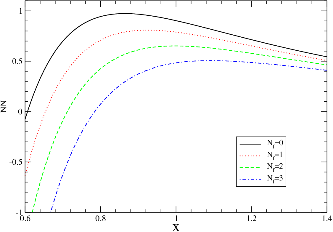
Considering the jump at five loop the uncertainty in this estimate can be too optimistic. To avoid such underestimation of the uncertainty we may also look at the renormalization scale dependence of the normalization constant. Being proportional to the gluon condensate the ratio
| (38) |
is scale independent, which means that the normalization of the series in powers of of the Adler function scales as
| (39) |
Thus the test of scale independence of
| (40) |
can give a hint of the reliability of the estimate (36). In Fig. 1 we see that is close to the scale of minimal dependence, and considering the variation of the normalization about it appears the error estimate in (36) is not unreasonable.
At this point it may be appropriate to isolate the universal portion of the normalization constants that is process-independent, by writing the normalization as
| (41) |
where denotes the leading order coefficient of the process-depedent Wilson coefficient for the operator . From the estimate of the normalization for the Adler function and (19) we obtain
| (42) |
The process-dependence of the normalization comes via , a short-distance quantity, and is the process-independent part of the normalization, which may be regarded as the long-distance contribution and an intrinsic property of the renormalon like the strength or the position of the renormalon singularity. That the process-dependence comes only via a short-distance quantity should not be surprising, considering that in IR renormalon diagrams the large order behavior arises from bubble chains of arbitrarily long, far-infrared region; hence all process-dependence should be a short-distance effect.
Now note that the normalization constant (37) is for the expansion in . For the usual power expansion in
| (43) |
the large order behavior is then given by
| (44) |
The plaquette coefficients were computed in numerical stochastic perturbation theory up to 20-loop orders [19, 20, 18]. At these orders the coefficients grow much faster than a renormalon behavior would suggest, and rather follow a power law. The plot (Fig.2) of the renormalon behavior (44) and power law [21] shows they meet at order . This may suggest the renormalon behavior would set in at orders around . Recently, the renormalon behavior in heavy-quark pole mass was confirmed in numerical simulation of the coefficients to order [14, 15]. Our estimate of the large order behavior of the plaquette suggests a numerical evidence of renormalon in plaquette would require much higher order computations.

Acknowledgements.
The author is deeply grateful to the theory group in the department of physics and astronomy at Johns Hopkins University and especially to Kirill Melnikov for hospitality. This work was supported by the overseas research program of Kunsan National University.References
- [1] J. C. Le Guillou and J. Zinn-Justin, Large order behavior of perturbation theory, Amsterdam, Netherlands: North-Holland (1990).
- [2] M. Beneke, Phys. Rept. 317, 1 (1999).
- [3] G. Parisi, Phys. Lett. B76, 65 (1978).
- [4] G. Parisi, Nucl. Phys. B150, 163 (1979).
- [5] F. David, Nucl. Phys. B234, 237 (1984).
- [6] F. David, Nucl. Phys. B263, 637 (1986).
- [7] A. H. Mueller, Nucl. Phys. B250, 327 (1985).
- [8] J. C. Collins, A. Duncan, and S. D. Joglekar, Phys. Rev. D16, 438 (1977).
- [9] M. Luscher and P. Weisz, Phys. Lett. B349, 165 (1995).
- [10] T. Lee, Phys. Rev. D56, 1091 (1997).
- [11] T. Lee, Phys. Lett. B462, 1 (1999).
- [12] A. Pineda, JHEP 06, 022 (2001).
- [13] T. Lee, Phys. Rev. D67, 014020 (2003).
- [14] C. Bauer, G. S. Bali, and A. Pineda (2011), eprint arxiv:1111.3946.
- [15] G. S. Bali, C. Bauer, and A. Pineda, PoS LATTICE2011, 222 (2011).
- [16] P. A. Baikov, K. G. Chetyrkin, and J. H. Kuhn, Phys. Rev. Lett. 101, 012002 (2008).
- [17] P. A. Baikov, K. G. Chetyrkin, and J. H. Kuhn, Phys. Rev. Lett. 104, 132004 (2010).
- [18] R. Horsley et al., PoS LATTICE2010, 264 (2010).
- [19] F. Di Renzo, E. Onofri, and G. Marchesini, Nucl. Phys. B457, 202 (1995).
- [20] F. Di Renzo and L. Scorzato, JHEP 10, 038 (2001).
- [21] R. Horsley, P. E. L. Rakow, and G. Schierholz, Nucl. Phys. Proc. Suppl. 106, 870 (2002).