Exact relaxation dynamics of a localized many-body state in the 1D Bose gas

Localized wave packets play a fundamental role in quantum mechanics, particularly, in the study of dynamical behavior. For a massive particle in a free space it is possible to construct a localized state such as Gaussian wave packets by superposing single-particle eigenfunctions, i.e., plane waves. When it evolves in time according to the Schrödinger equation, the wave packet collapses due to the uncertainty relations [1]. For interacting many-body systems, on the other hand, it is in general a formidable task to pursue the unitary time evolution for a given initial state over a sufficiently long time with satisfactory accuracy [2]. It is even elusive how to define and construct an initially localized state of a physical meaning in a system with translation symmetry.

The quantum dynamics of interacting many particles has recently attracted much interest associated with the question of “relaxation” and “thermalization” of isolated systems [3]. In order to understand the concept of relaxation von Neumann’s ergodic theorem should be useful [4, 5, 6, 7]. Furthermore, relaxation dynamics after a sudden quench has been studied for integrable systems [8]. In the studies it is also essential to well define an initial state. Recent experiments in cold atoms [9] enable us to study the isolated quantum dynamics of initially localized states because of the high isolation from the environment and controllability of system parameters. Thus it is of importance to theoretically explore how to describe a localized state and to track its long-time behavior, in both integrable and nonintegrable systems.

In this Letter, we show that a localized many-body state with a density notch is constructed by superposing the Bethe ansatz eigenstates of a certain type for the 1D interacting Bose gas with repulsive delta-function potentials. They are given by a series of one-hole excitations, which are called Lieb’s type II excitations [10]. In the weak coupling case, the initial density profile is quite similar to the graph of the squared amplitude of a dark soliton, which is a solution of the nonlinear Schrödinger equation for the classical scalar field. We numerically solve the exact time evolution of the expectation value of the density operator. Observing the movies of the density profile, we find that the system with $N=1000$ shows relaxation dynamics as if it were thermodynamically large, while that with $N=20$ shows finite-size effects such as recurrence phenomena. The relaxation time of the broken symmetry state resembling a dark soliton increases in the weak coupling case. Thus, the localized wave packets are more stable as the constant $c$ becomes smaller, which suggests the existence of off-diagonal long-range order.

Let us consider the Hamiltonian of the 1D interacting bosons with repulsive delta-function potentials, called the Lieb-Liniger (LL) model [10]:

Here we assume the periodic boundary conditions of the system size $L$ on the wavefunctions. Hereafter we consider the repulsive interaction: $c>0$. The LL model is characterized by a single parameter $\gamma:=c/n$, where $n=N/L$ is the density of the particles. We fix the particle density as $n=1$ and vary the coupling constant $c$. We employ a system of units with $2m=\hbar=1$. The unit of time in our simulation is proportional to $L^{-2}$.

In terms of the canonical Bose field $\hat{\psi}(x,t)$, the LL model corresponds to ${\cal H}_{\text{NLS}}=\int_{0}^{L}dx[\partial_{x}\hat{\psi}^{\dagger}\partial_{x}\hat{\psi}+c\hat{\psi}^{\dagger}\hat{\psi}^{\dagger}\hat{\psi}\hat{\psi}].$ The second quantized Hamiltonian ${\cal H}_{\text{NLS}}$ leads to the nonlinear Schrödinger equation for the canonical Bose field: $i\partial_{t}\hat{\psi}=-\partial^{2}_{x}\hat{\psi}+2c\hat{\psi}^{\dagger}\hat{\psi}\hat{\psi}\,.$

In the weak coupling limit ($c\to 0$), the one-particle reduced density matrix is well approximated by the macroscopic wavefunctions: $\rho_{1}(x,y)\simeq\Psi^{*}(x)\Psi(y)$, where $\Psi(x)$ is the eigenfunction corresponding to the maximum eigenvalue of $\rho_{1}(x,y)$. In fact, we can numerically show that the largest eigenvalue of $\rho_{1}$ is much larger than the other eigenvalues for small $c$, which suggests the existence of off-diagonal long-range order. The density operator $\rho(x)$ is defined by the diagonal elements of the one-particle reduced density matrix: $\rho(x)=\rho_{1}(x,x)$.

There is a well-known conjecture claiming that, in the weak coupling limit, the 1D Bose gas, which is a quantum integrable system, should become a classical integrable system, which is described by the Gross-Pitaevskii equation, i.e., the nonlinear Schrödinger equation for the classical scalar field. It was addressed that the mode of classical dark solitons is identified with the type II excitations of the LL model through the coincidence of their dispersion relations in the weak coupling limit [11]. However, it is still nontrivial to show how the classical solitons are derived from the 1D interacting bosons with $c>0$ even in the weak coupling limit. For the attractive case ($c<0$), this was studied analytically [12]. Through numerical simulation, the quantum dynamics of dark solitons in the optical lattice system has been investigated for the Bose-Hubbard model [13]. The type II excitations are interpreted as quantum solitons in association with yrast states [14].

In the LL model, the Bethe ansatz offers an exact eigenstate with an exact energy eigenvalue for a given set of quasimomenta $k_{1},k_{2},\ldots,k_{N}$ satisfying the Bethe ansatz equations for $j=1,2,\ldots,N$:

Here $I_{j}$’s are integers for odd $N$ and half-odd integers for even $N$. We call them the Bethe quantum numbers. The total momentum $P$ and energy eigenvalue $E$ are written in terms of the quasimomenta as $P=\sum_{j=1}^{N}k_{j}=\frac{2\pi}{L}\sum_{j=1}^{N}I_{j}$, $E=\sum_{j=1}^{N}k_{j}^{2}$. If we specify a set of the Bethe quantum numbers $I_{1}<\cdots<I_{N}$, Bethe ansatz equations (2) have a unique real solution $k_{1}<\cdots<k_{N}$ [15]. In particular, the sequence of the Bethe quantum numbers of the ground state is given by $I_{j}=-(N+1)/2+j$ for integers $j$ with $1\leq j\leq N$. The Bethe quantum numbers for low lying excitations are systematically derived by putting holes or particles in the ground-state sequence.

Let us now construct an initial state with a localized density profile. In the type II branch, we denote by $|P\rangle$ the normalized Bethe eigenstate of total momentum $P=2\pi p/L$ for each integer $p$ in the set $\{0,1,\ldots,N-1\}$. The Bethe quantum numbers of $|P\rangle$ are given by $I_{j}=-(N+1)/2+j$ for integers $j$ with $1\leq j\leq N-p$ and $I_{j}=-(N+1)/2+j+1$ for $j$ with $N-p+1\leq j\leq N$. For each integer $q$ satisfying $0\leq q\leq N-1$, we define the coordinate state $|X\rangle$ of $X=qL/N$ by the discrete Fourier transformation:

It turns out, remarkably, that the density profile of $|X\rangle$ has a density notch at the position $X+L/2$ as shown in the top panels of Figs. 1, 2, and 3. In the simulation we put $q=0$, and the initial density profile $\rho(x)$ is localized at $x=L/2$. The “temperature” of the state $|X(t)\rangle$ is estimated by equating the mean energy of the state with the internal energy derived from the thermodynamic Bethe ansatz [16], although it is not in thermal equilibrium.

The construction is analogous to the analysis of the attractive case ($c<0$) in which the Fourier transformation of the $n$-particle bound state $|n,P\rangle$ with momentum $P$ gives a localized state $|n,X\rangle$ with the center of mass located at $X$, and the matrix element of the field operator $\langle n,X^{\prime}|\hat{\psi}(x,t)|n+1,X\rangle$ exactly corresponds to a bright soliton solution of the nonlinear Schrödinger equation for the classical scalar field with $c<0$ [12].

Let us introduce $|X(t)\rangle=\exp(-i{\cal H}t)|X\rangle$. We evaluate the expectation value at time $t$ of the density operator $\rho(x)=\hat{\psi}^{\dagger}(x)\hat{\psi}(x)$ for the initial state $|X\rangle$ as

where $P=2\pi p/L$ and $P^{\prime}=2\pi p^{\prime}/L$ denote the total momenta of the normalized Bethe eigenstates $|P\rangle$ and $|P^{\prime}\rangle$, respectively.

Because of quantum integrability, we numerically obtain all the energy eigenvalues $E_{p}$ of $|P\rangle$’s in the type II branch and follow the time evolution for quite a long time.

We evaluate the form factor $\langle P^{\prime}|\rho(0)|P\rangle$ in Eq. (4) through Slavnov’s formula [17] together with the Gaudin-Korepin formula [18] for the norm of the Bethe eigenstate as

where the quasimomenta $\{k_{1},\cdots,k_{N}\}$ and $\{k^{\prime}_{1},\cdots,k^{\prime}_{N}\}$ give the eigenstates $|P\rangle$ and $|P^{\prime}\rangle$, respectively. We use the abbreviations $k_{j,\ell}:=k_{j}-k_{\ell}$ and $k^{\prime}_{j,\ell}:=k^{\prime}_{j}-k^{\prime}_{\ell}$. The kernel $K(k)$ is defined by $K(k)=2c/(k^{2}+c^{2})$. The matrix $G(k)$ is the Gaudin matrix, whose $(j,\ell)$ th element is $G(k)_{j,\ell}=\delta_{j,\ell}\left[L+\sum_{m=1}^{N}K(k_{j,m})\right]-K(k_{j,\ell})$ for $j,\ell=1,2,\cdots,N$. The matrix elements of the $(N-1)$ by $(N-1)$ matrix $U(k,k^{\prime})$ are given by

We thus numerically solve the exact time evolution of the density profile: Once we evaluate the form factors at $t=0$ we obtain the density profile at any late time $t$ by taking only the sum of exponentials [19]. Through Eq. (5), the evaluation of the form factors of the Bethe eigenstates with $N$ particles is reduced to that of the determinants of $N$ by $N$ matrices.

The density profile of a wave packet for $N=1000$ initially has a localized shape without translation symmetry, and then it relaxes into a flat profile in equilibrium through time development, as shown in Figs. 1 and 2. The relaxation time increases as the constant $c$ decreases.

In the weak coupling case of $c=0.01$, the density profile is smooth and its time evolution is very slow as shown in Fig. 1. The density profile maintains a featureless curve through the time development and has a long coherence in space suggesting the existence of off-diagonal long-range order.

We observe that the initial density profile for $c=0.01$ overlaps the plot of the squared amplitude of a dark soliton solution of the nonlinear Schrödinger equation for the classical scalar field. This observation is fundamental for making an explicit connection between the type II excitations and the dark solitons. We shall discuss this in detail in a separate publication.

In the strong coupling case of $c=100$, the time evolution is much faster. The initial density profile also shows small oscillating behavior at the shoulders of the density notch, which are similar to the Friedel oscillations of the Fermi gas. The initial wave packet dynamically splits into many fragments, which results from the strong repulsive interaction. The initial density profile is rather different from the graph of the squared amplitude of a dark soliton.

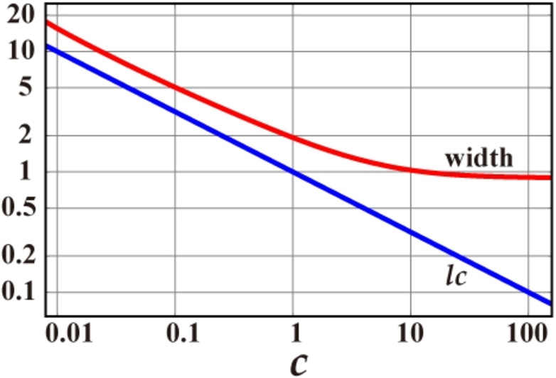
The width of the initial density notch is approximately proportional to the healing length $\ell_{c}$ for small $c$, as is the case for the classical dark soliton (see Fig. 4). For larger $c$, however, it seems that the width does not decrease in proportion to $\ell_{c}$. This suggests the existence of fermionic hard cores.

Let us calculate the Loschmidt echo, i.e., the fidelity. We define it by the overlap between the initial state $|X(0)\rangle$ and the time-evolved state $|X(t)\rangle$ at time $t$ as

We plot the Loschmidt echo in Fig. 5 with fixed particle density $n=N/L=1$ in the strong coupling case of $c=100$.

For a large system size ($N=1000$), as shown in the left panel of Fig. 5, it decays almost monotonically with the short-time fluctuations being rather small. This behavior is common for a wide range of values of $c$ with different scales of time. In the strong coupling limit $c\to\infty$, by sending $N$ and $L$ to $\infty$ with fixed density $n=N/L$ we derive analytical forms of the Loschmidt echo: $F(t)=[C(n\sqrt{2\pi t})^{2}+S(n\sqrt{2\pi t})^{2}]/(2\pi n^{2}t)$, where $C(x)$ and $S(x)$ are given by the Fresnel integrals defined by $C(x):=\int_{0}^{x}\cos(\pi s^{2}/2)ds$ and $S(x):=\int_{0}^{x}\sin(\pi s^{2}/2)ds$, respectively. As a short-time expansion we have $F(t)=1-4\pi^{4}n^{4}t^{2}/45+\mathcal{O}(t^{3})$, and as a long-time expansion we have $F(t)=(4\pi n^{2}t)^{-1}+\mathcal{O}(1/t^{2})$. The plot of numerical results for $N=1000$ with $c=100$ (left panel of Fig. 5) almost overlaps that of the analytical expression of the Fresnel integrals. It suggests that the system of $N=1000$ already shows thermodynamic behavior.

For a small system size ($N=20$) the Loschmidt echo is shown in the right panel of Fig. 5. Here, we observe large fluctuations due to the finite-size effect.

Let us define a long-time average $\mathbb{E}$ by $\mathbb{E}[f(t)]:=\lim_{T\to\infty}\int_{0}^{T}dtf(t)/T$. Using $\mathbb{E}[e^{i\omega t}]=0$ for $\omega\neq 0$ and $\mathbb{E}[e^{i\omega t}]=1$ for $\omega=0$, we obtain $\mathbb{E}[F(t)]\sim 1/N$ for any value of $c$. This is also confirmed by our simulation.

A sharp peak at $t\simeq 33$ in the Loschmidt echo for $N=20$ shows the signal of a recurrence phenomenon. In fact, the localized wave packet is revived at this time after a “tentative” relaxation as shown in Fig. 3.

In conclusion we have shown that the superposition of the Bethe eigenstates of the type II excitations leads to a quantum many-body state with a localized density profile. It perfectly overlaps the plot of the squared amplitude of a dark soliton in the weak coupling regime. By means of Slavnov’s formula together with the Gaudin-Korepin formula, we have numerically solved the exact time evolution of the density profile in both the strong and weak coupling cases for a large number of particles such as $N=1000$ over a very long period of time. For a sufficiently large system size ($N=1000$), we observe that a density profile with broken translation symmetry relaxes into a flat profile in equilibrium through the time development. For a small system size ($N=20$), the localized wave packet is revived after a tentative relaxation. These observations suggest that the method presented in this Letter should be fundamental for exploring exact approaches to the quantum dynamics of many-body systems.

The authors thank I. Danshita and K. Sakai for their useful discussions. The present research is partially supported by Grant-in-Aid for Scientific Research No. 21710098. J.S. is supported by JSPS.

References

- [1] J.J. Sakurai, Modern Quantum Mechanics, ed. by S. F. Tuan, (Addison-Wesley Publ. Co., 1994).
- [2] Q.Y. He, M.D. Reid, B. Opanchuk, R. Polkinghorne, Laura E. C. Rosales-Zarate, P.D. Drummond, arXiv:1112.0380 .
- [3] M. Rigol, V. Dunjko, V. Yurovsky and M. Olshanii, Phys. Rev. Lett. 98, 050405 (2007); M. Rigol, V. Dunjko and M. Olshanii, Nature 452, 854 (2008).
- [4] R. Tumulka, arXiv:1003.2133, English translation of J. von Neumann: Zeitschrift fur Physik57, 30-70 (1929).
- [5] S. Goldstein, J.L. Lebowitz, C. Mastrodonato, R. Tumulka and N. Zhanghi, Proc. Roy. Soc. A 466, 3203 (2010).
- [6] H. Tasaki, An observation based on the works by Goldstein, Lebowitz, Mastrodonato, Tumulka and Zhanghi in 2009, and by von Neumann in 1929, arXiv:1003.5424
- [7] T. Monnai, Phys. Rev. E 84, 011126 (2011).
- [8] A. Faribault, P. Calabrese and J.-S. Caux, J. Math. Phys. 50, 095212 (2009); J. Mossel, G. Palacios and J.-S. Caux, J. Stat. Mech., L09001 (2010); J. Mossel and J.-S. Caux, New J. Phys. 12, 055028 (2010).
- [9] T. Kinoshita, T. Wenger and D.S. Weiss, Nature 440, 900 (2006).
- [10] E.H. Lieb and W. Liniger, Phys. Rev. 130, 1605 (1963); E.H. Lieb, Phys. Rev. 130, 1616 (1963).
- [11] M. Ishikawa and H. Takayama, J. Phys. Soc. Jpn. 49, 1242 (1980).
- [12] C.R. Nohl, Ann. Phys. 96, 234 (1976); M. Wadati, M. Sakagami, J. Phys. Soc. Jpn. 53, 1933 (1984); M. Wadati, A. Kuniba, T. Konishi, J. Phys. Soc. Jpn. 54, 1710 (1985); M. Wadati, A. Kuniba, J. Phys. Soc. Jpn. 55, 76 (1986).
- [13] R.V. Mishmash and L.D. Carr, Phys. Rev. Lett. 103, 140403 (2009); R.V. Mishmash, I. Danshita, C.W. Clark and L.D. Carr, Phys. Rev. A 80, 053612 (2009).
- [14] R. Kanamoto, L.D. Carr, M. Ueda, Phys. Rev. A 81, 023625 (2010).
- [15] V.E. Korepin , N.M. Bogoliubov and A.G. Izergin, Quantum Inverse Scattering Method and Correlation Functions (Cambridge University Press, Cambridge, 1993)
- [16] C.N. Yang and C.P. Yang, J. Math. Phys. 10, 1115 (1969).
- [17] N. A. Slavnov, Teor. Mat. Fiz. 79, 232 (1989) ; 82, 389 (1990); J.-S. Caux, P. Calabrese and N. A. Slavnov, J. Stat. Mech. P01008 (2007).
- [18] M. Gaudin, “La fonction d’onde de Bethe”, Masson (Paris) (1983); V. E. Korepin, Commun. Math. Phys. 86, 391 (1982).
- [19] We have solved Bethe ansatz equations (2) with errors of given by and obtain energy eigenvalues with errors of . Therefore, the accuracy of the time evolution is assured as long as .