Average Interpolation Under
the Maximum Angle Condition
Abstract
Interpolation error estimates needed in common finite element applications using simplicial meshes typically impose restrictions on the both the smoothness of the interpolated functions and the shape of the simplices. While the simplest theory can be generalized to admit less smooth functions (e.g., functions in rather than ) and more general shapes (e.g., the maximum angle condition rather than the minimum angle condition), existing theory does not allow these extensions to be performed simultaneously. By localizing over a well-shaped auxiliary spatial partition, error estimates are established under minimal function smoothness and mesh regularity. This construction is especially important in two cases: estimates for data in hold for meshes without any restrictions on simplex shape, and estimates for data in hold under a generalization of the maximum angle condition which requires for standard Lagrange interpolation.
Interpolation error estimates for the standard finite element spaces typically involve two requirements: conditions on the smoothness of the function being interpolated (data regularity) and constraints on the geometry of the elements of the mesh (shape regularity). Beyond the simplest interpolation error estimates (stated precisely in Proposition 1.2), data or shape regularity can be substantially relaxed with some additional analysis. However the existing theory does not accept the weakest restrictions on both data and shape regularity simultaneously.
Data Regularity and Average Interpolation
Lagrange interpolation involves point-wise function evaluation leading to data regularity restrictions associated with the requirements of the Sobolev embedding theorem. Alternatively, average interpolation can be used to handle less regular data [13, 38, 5, 37, 11]. Because average interpolation ‘smears’ local estimates over a neighborhood of simplices, error estimates rely more heavily on the geometry of the mesh, often needing meshes of bounded ply (defined in Section 1.3, see Figure 1) so global summation can be performed.
Shape Regularity and Angle Conditions
For triangular meshes the classical error estimates are typically proved under a minimum angle restriction, but this condition is overly restrictive. Triangle geometry and interpolation error are actually related through the largest angle of the triangle [43, 6, 22]. (Convergence of the finite element method can occur for meshes with arbitrarily large angles [8, 19], but the known counterexamples are finite element spaces containing subspaces associated with a shape regular mesh.) The maximum angle condition can be generalized to higher-dimensional simplices but existing analysis gives stronger data regularity requirements [22, 24, 39]. The linear tetrahedral element is especially important to this discussion. Shenk constructed a counterexample demonstrating that the expected Lagrange interpolation error estimates do not hold for a fairly innocuous family of narrow tetrahedra [39]; see Fig. 3(right). Analysis using an average interpolant eliminates this problem but again leads to new geometric restrictions on the ply of the mesh [1].
Mesh Generation
Geometric restrictions needed to prove interpolation error estimates are essentially the output requirements for a mesh generator. In 2D many mesh generation techniques aim to produce bounded aspect ratio triangulations (although a notable exception [30] only removes large angles), but aspect ratio guarantees are impossible when the input (i.e., the boundary of the domain) contains small angles [40]. To admit arbitrary input several mesh generation strategies have been developed which allow a few poor quality triangles near small input angles [29, 33, 40, 36]. Guided by the interpolation theory the most commonly used strategy [29] provides provable upper bounds on the largest angle and the ply of the mesh (as long as the input does not include high degree vertices). This effective approach does not extend to 3D and guaranteed mesh generation algorithms do not yield a bound on the ply [25, 42, 41, 10, 35, 36]. Figure 2(left) demonstrates the high ply construction in the analogous 2D algorithm. Failures of these algorithms are difficult to observe in practice since the mesh ply only grows logarithmically in the (inverse of the) size of the smallest angle, but they represent a theoretical disconnect between output guarantees of the mesh generator and the input requirements of numerical methods. Beyond provably-correct mesh generation algorithms, simplified mesh generation algorithms are often practically successful, and allowing high ply meshes extends the range of inputs producing acceptable results. Uniform refinement of a structured grid in polar coordinates is perhaps the simplest situation yielding a high ply node; see Figure 2(right). Providing the loosest set of geometric requirements in the interpolation theory gives mesh generators the most flexibility in practical applications as well as new challenges to improve existing guarantees under weaker requirements.
Outline
This paper demonstrates that there is no inherent trade-off between data regularity and shape regularity in interpolation of less regular Sobolev functions on simplicial meshes by developing a theory accepting minimal data and shape regularity requirements. The key insight is that error estimates cannot be localized over the meshes of high ply; rather a simpler auxiliary spatial partition must be used. Before describing this construction, Section 1 contains the necessary preliminary discussion including a more formal exposition of the prior results. Error estimates for the average interpolant under uniform size and quality meshes are shown in Section 2. A generalization to non-uniform meshes is given in Section 3 before some concluding remarks in Section 4.
1 Preliminaries

|

|

|

|
![[Uncaptioned image]](1112.4100v2/smallangle2.png)
|
![[Uncaptioned image]](1112.4100v2/polarrefinement.png)
|
The statement is used to mean there exists a positive constant such that when the details of the constant are unimportant. For nearly all estimates discussed, this implied constant will be independent of simplex/mesh shape regularity; whenever this is not the case, it will be explicitly noted.
1.1 Balls, Cubes, and Simplices
The ball of radius centered at is the set of points with Euclidean distance from less than :
A -cube or cube is a closed set of the form
The point is called the center of and is called the size of , denoted . A simplex is the convex hull of non-coplanar points (called vertices), :
We let denote the length of the longest side of and denote the radius of the largest sphere inscribed in . Following Jamet’s shape regularity condition [22], the angle is defined to characterize the quality of a simplex by the formula,
| (1) |
where is the set of unit vectors parallel to the edges of the simplex ; see Fig. 3. This angle measures how far from coplanar the set of edges is, so we call the coplanarity measure. The subscript on , , and is often omitted when the simplex in question is apparent. In two dimensions is half the largest angle of the triangle, and thus the set of triangles with coplanarity bounded away from satisfy the maximum angle condition in the sense that all angles are bounded away from . In three dimensions, a more intuitive generalization of the maximum angle condition defined by defined by Křížek [24] requires that both face and dihedral angles of the tetrahedron are bounded away from . This is also equivalent to bounding coplanarity away from as shown in the proposition below.
Proposition 1.1.
Let denote the maximum of all face and dihedral angles of (three-dimensional) tetrahedron . For tetrahedra, bounds on coplanarity and face/dihedral angles are equivalent, i.e., if is bounded away from then is bounded away from and vice versa.
The proof, given in Appendix A, relies on a characterization of tetrahedra satisfying the maximum angle condition given in [2].

1.2 Sobolev Spaces
We will distinguish between the notation and . The former will be used to denote differentiation with respect to a particular variable while the latter represents differentiation with respect to a function argument. For example, the following notation is used for an application of the chain rule:
The Sobolev semi-norms and norms on functions over an open set are defined by
where the first summation is taken over multi-indices and differentiation with respect to multi-indices has the standard definition, . The -norm is simply the standard -norm.
Throughout this paper, is a bounded set and an extension domain for any Sobolev spaces used; i.e. there is a continuous, linear operator such that for all ; see [3, p. 83] for technical results concerning extension domains. Without ambiguity, the functions and will not be distinguished: for , denotes . Likewise, the estimate is used freely.
1.3 Lagrange Interpolation on Simplicial Meshes
always denotes a simplicial mesh of . The ply of the mesh is the maximum number of mesh simplices intersecting a single simplex. Ply restrictions are often implicit in interpolation error estimates since a mesh with bounded aspect ratio has a bounded ply. (In fact, the weaker restriction of bounded circumradius to shortest edge ratio is sufficient to ensure bounded ply [44, 21].)
Let denote the -th degree Lagrange interpolant on a simplicial mesh,
where are the piecewise nodal basis functions on . While this paper only considers linear interpolants (), the higher order cases are included in the statement of classical estimates for smooth functions.
1.4 Prior Interpolation Error Estimates
The Bramble-Hilbert Lemma [7, 14] along with scaling properties of Sobolev semi-norms leads to the following classical error estimate for the Lagrange interpolant; see [12, 15, 9] for complete details.
Proposition 1.2.
If and , then for all simplices and all ,
| (2) |
For simplices with bounded aspect ratio, and are proportional and thus the factor reduces to . The estimate in the -norm (i.e., the case) is particularly nice: the term in the denominator disappears and the estimate is independent of the shape of the simplex.
The first generalization involves weakening the data regularity requirement, i.e., the restriction . A function (but not in ) is not necessarily continuous so an alternative to Lagrange interpolation must be considered. Clément first described such an interpolant and proved an estimate which corresponds to the ()-case of (2) [13]. Scott and Zhang proved a similar estimate based on an average interpolant [38]: specifically interpolant values at mesh vertices are defined to be averages over an arbitrarily selected adjacent simplex. A distinct advantage of the Scott and Zhang interpolant is that coefficients of basis functions corresponding to boundary nodes only depend upon the boundary data. An alternative approach based on averaging over balls has been developed which extends to vector-valued functions in the discrete de Rham complex [5, 37, 11]; see Figure 4 for a comparison of the averaging regions. The resulting interpolant of Christiansen and Winther also matches homogeneous boundary data selecting an appropriate extension of the function outside the domain. In the simplest case, each of these constructions reduces to the following theorem.
Theorem 1.3 (Specialized from [38, 11], etc.).
Suppose has a bounded aspect ratio and let be an average interpolant. Then for all ,
| (3) |
where is the union of and its neighboring simplices.
Unlike the (, )-case of Proposition 1.2, Theorem 1.3 requires a bounded aspect ratio mesh ensuring two things. First, and its neighboring simplices have roughly the same size so that . Second, has a bounded ply so these local estimates (3) over each simplex can be summed to a global estimate. Our aim is to remove these restrictions on simplex shape to match the case of the classical estimate (2) which is independent of simplex shape.
The second generalization of Proposition 1.2 weakens the shape regularity requirements. For this purpose, Jamet developed an improved estimate for sufficiently regular data.
Theorem 1.4 (Jamet, [22]).
If , then for all ,
| (4) |
The restriction prevents Jamet’s result from applying in certain cases including (perhaps the most important cases of) linear interpolation on triangles and tetrahedra: when or . The analysis of Babuška and Aziz [6] yields the result for the linear triangular element (although care must be taken to derive the correct geometric factor using this approach [23, 18, 28, 34]). Shenk generalized the approach of Babuška and Aziz to higher dimensions and, more importantly, demonstrated that (4) does not hold for the linear Lagrange interpolant on tetrahedra [39]. Shenk’s example involves particularly simple geometry: a family of tetrahedra depicted in Figure 3 with vertices , , , and where approaches zero. Demonstrating the error estimate for an analogous class of triangles (i.e., 2D simplices) is the crux of the argument of Babuška and Aziz.
An analysis by Acosta demonstrated that expected error estimates can be extended to certain narrow tetrahedra (including those in Shenk’s example) by using average (rather than Lagrange) interpolation [1]. This method does allow data and shape regularity to be weakened simultaneously, but the analysis is inherently anisotropic: locally it must be possible to affinely transform the mesh into a shape-regular mesh. (This is a standard requirement in an anisotropic framework; e.g., [4, 17, 20].) The resulting estimates expect the mesh to have a bounded ply so that local estimates can be summed to form global error estimates. Note that the meshes in Figure 2 do not satisfy the requirements of [1].
We will develop interpolation error estimates based on average interpolation under weakened data and shape regularity requirements. Emphasis will be placed on avoiding any unnecessary element shape requirements which, most notably, allows meshes with unbounded ply (as is the case for Lagrange interpolants in Theorem 1.4). The result will be an interpolation theory which extends Jamet’s minimal shape regularity requirements to less smooth data including the linear tetrahedral element.
2 Uniform Error Estimates
To avoid the limitations associated with pointwise function evaluation, an average interpolant is defined by mollifying the data before Lagrange interpolation:
| (5) |
In the next subsection, the standard mollification procedure is defined and a number of needed properties are given.
Remark 2.A. This interpolant is used in [5, 37, 11], but in that context, the mollification radius was selected to be small enough so that the averaging region stays within the neighboring triangles. Since we do not assume aspect ratio bounds, we cannot use this property. Acosta uses essentially an anisotropic variant of this construction [1]; see Figure 4.

2.1 Mollification and Integration
Mollification is a common tool in analysis for producing smooth approximations of functions in spaces. After defining the procedure, a few common facts about mollification are listed. The proofs of these and similar results can be found in a number of textbooks, but are given in the appendix for comparison to the later sections. For some examples of these kinds of technical details, especially those for more regular data and including explicit dependence on on the mollification radius, see [32, p. 191], [26, p. 58], [27, p. 98], and [16, p. 201].
Let such that (i) , (ii) , and (iii) for all . Let . Then, (i) , (ii) , (iii) for all , and (iv) . The most commonly used mollifier is where the constant is chosen so (ii) holds. We also require that is radially symmetric. While symmetry is not usually required, the common mollifier is symmetric and we explicitly use the property in one step of the upcoming arguments.
A function is mollified by convolving it with : given , define
The two representations above are equivalent, resulting from a simple change of variables, , but the supports of the integrands are different. If a function is smooth enough (specifically, it belongs to in the proposition below) then the difference between the function and its mollification can be bounded in terms of the mollification radius.
Proposition 2.1.
If , then for all ,
The next proposition demonstrates how the smoothness of the mollifier depends on the mollification radius through a bound on the -norm of a mollified function in terms of the -norm of the original function.
Proposition 2.2.
If and is a bounded set, then for all ,
| (6) |
where .
Remark 2.B. Since , Proposition 2.2 also applies for higher Sobolev norms; specifically, (6) implies that
| (7) |
Finally a standard estimate of the -norm of a function in terms of the -norm is stated for larger than . This can be proved with either Jensen’s or Hölder’s inequality.
Proposition 2.3.
If and is a bounded set, then for all ,
2.2 Error Estimate
Next we turn to removing the integrability condition in Jamet’s estimate (4). Again for simplicity we first consider meshes in which simplex size and quality (measured by coplanarity, not aspect ratio) are uniformly bounded and then relax these assumptions in Section 3.
Theorem 2.4.
Suppose contain no edges longer than and let be the maximum simplex coplanarity. Then for and for all ,
| (8) |

Proof.
First the triangle inequality is applied using the intermediate function ,
| (9) |
The first term of (9) is independent of the triangulation and is estimated using Proposition 2.1:
| (10) |
Next the second term of (9) is addressed:
| (11) |
The estimate is established locally, but not over the individual simplices of . This is important since averaging ‘smears’ the estimate on one simplex over its neighbors. Since we allow for high ply meshes, it is not possible to sum these local estimates to yield the global result (8). Rather, the estimate is localized over a simple artificial (and bounded-ply) decomposition, a covering of by cubes.
In a lattice of cubes of side-length , let be the subset which intersect ; see Figure 5. The term (11) is estimated on a single cube . Let and denote the cubes of side-length and , respectively, centered around , and let be the set of simplices in the triangulation which intersect ; see Figure 6.
Next a value is selected arbitrarily with the intention of applying Theorem 1.4 (since we are in the setting ). Applying Proposition 2.3 followed by the definition of yields,
Theorem 1.4 can now be applied to each term of the summation on the right hand side and Proposition 2.2 is used to return the estimate to the correct norm:
Since , we conclude that
| (12) |
Finally these estimates can be summed to get the global estimate:
| (13) |
The final inequality holds since each cube belongs to at most cubes . ∎

Remark 2.C. The essential difference between this analysis and that of Acosta [1] is the use of the artificial (and bounded-ply) mesh for establishing the local estimate (12).
Remark 2.D. Looking closely at the inequality (13) reveals that the extension domain property has been used to estimate by .
Remark 2.E. In the case of (8), i.e, , the estimate does not depend on simplex shape which agrees with the classical result for more regular data.
3 Locally Quasi-Uniform Error Estimates
Extending Theorem 2.4 to admit non-uniform meshes requires a precise characterization of the mesh size at each point in the domain. We emphasize that the size function does not necessarily reflect the size of the triangles in the mesh. Rather it is only an upper bound. Because the average interpolant depends on a local neighborhood, the sizing function should not vary too rapidly so that there is roughly a unique size (up to a constant factor) associated with the neighborhood.
Before proving error estimates, we outline precise restrictions on these sizing functions. Then based on the sizing function, variable-radius mollification and compatible cubic coverings are defined. As before, the final interpolation operator is a composition of the (modified) mollification operation with the usual Lagrange interpolation operator :
| (14) |
3.1 Sizing Function
Using Lagrange interpolation for smooth (enough) functions, mesh size is captured locally by the length of the longest edge of a given triangle. For average interpolation, function values over neighboring triangles must be considered and thus the size of the averaging region also plays a role in the error estimate. On bounded aspect ratio meshes this is not an issue since the longest edges of any pair of neighboring triangles are within a constant factor [31]. To analyze average interpolants for meshes without aspect ratio bounds, we decouple the mesh sizing function from the actual size of the triangles. Rather, the sizing function will be a smooth (enough) function which provides an upper bound on the size of nearby triangles in the mesh. The result will be a sizing function which can be used in the error estimate despite admitting meshes with adjacent triangles with dramatically different sizes.
Letting be a positive constant, we consider the class of sizing functions with bounded first and second derivatives:
| (15) |
| (16) |
We call a triangulation of compatible with sizing function if for all , where denotes the triangle containing .11 1 Without causing confusion this is a slight abuse of notation using to denote the sizing function and to denote the length of the longest edge of triangle. This is done to emphasize the fact that the sizing function plays the role of the mesh size in the upcoming estimates. In this setting, we will establish uniform interpolation estimates for any sizing function with a compatible mesh as long as the sizing function satisfies (15) and (16) and the mesh satisfies the maximum angle condition (in the sense of coplanarity).
Remark 3.A. The particular choice of constant in (15) is not essential. However, this value is very convenient for localizing future estimates to one layer of neighboring cubes in a 2:1 balanced cubic partition described in Subsection 3.3. Selecting a larger constant in (15) will require analysis of more levels of the cubic partition.
Remark 3.B. Restriction (15) is implicitly present (although the constant is often weaker) in the context of shape regular meshes. For a shape-regular mesh and letting be the union of triangles in which intersect triangle , we define
This definition of can be extended to using linear interpolation over the triangulation and it immediately follows that the triangulation is compatible with . Moreover, properties of well-spaced point sets ensure that can be bounded depending only on the mesh shape regularity [31, 44, 21]. In other words, a shape regular mesh can be viewed as a mesh that is compatible with a Lipschitz sizing function, and thus (16) is the only extra condition on the sizing function we require to handle less shape-regular meshes.
Remark 3.C. Restrictions (15) and (16) do allow for non-uniform meshes. The sequence of sizing functions can be paired with a sequence of meshes with progressively smaller elements near the origin. However, (16) does pose some additional limitations on how quickly the sizing function can approach zero: in the shape regular case common adaptive refinement matches a sizing function or which is not smooth enough for (16). See Figure 7.

 |

 |
Remark 3.D. Restrictions (15) and (16) are somewhat weaker than those used in [1] where there are restrictions essentially of the form . In that setting Gronwall’s inequality prevents such sizing functions from being truly non-uniform. Using the techniques of this paper, it should be possible to recover Acosta’s anisotropic results in a similar relaxed setting.
3.2 Variable-Radius Mollification
We now consider the generalization of mollification by allowing the mollification radius to vary over the domain. Given and sizing function , define
The only difference between this definition and the standard mollifier is that the radius is spatially varying. We consider an isotropic mollification region (and thus produce isotropic error estimates). The prior construction of Acosta uses an anisotropic mollifier, i.e., the term replaces in the above definition [1]. First we note a simple property of the variable radius mollifier.
Proposition 3.1.
Let and , and define . Then for all the sizing functions satisfying (15) and for all ,
| (17) |
Proof.
Extensions of Propositions 2.1 and 2.2 are necessary to prove the non-uniform error estimates. Since Remark 2.B no longer applies, i.e.,
we prove these lemmas directly in the correct Sobolev norms.
Lemma 3.2.
Let and be a cube. Then for and for all ,
| (18) |
where , and .
Proof.
The case of inequality (18) follows from a very similar argument to the proof of Proposition 2.1. Letting be an arbitrary function,
Next we note that and then bound the inner integral independent of by expanding the set :
Note: the construction was used to eliminate the integral in the variable. Selecting completes the result.
Next, the case of inequality (18) is addressed. We begin by computing directly:
| (19) |
Then letting ,
| (20) |
The first term can be estimated using the argument applied to (18) yielding,
| (21) |
It only remains to estimate . Let denote the halfspace with positive first coordinate, . First is rewritten in terms of second derivatives of :
Our selection of a radially symmetric mollifier is important above as the property has been applied.
where denotes the Hessian of , the matrix of second derivatives. Next, Hölder’s inequality can be applied:
| (22) |
Finally setting , and then combining (22) with (21) completes the result. ∎
The next step is to develop an extension of Proposition 2.2 for the variable-radius mollifier.
Lemma 3.3.
Proof.
We begin with the case . For all ,
The previous inequality results from a change of variables . (Note, is fixed in this transformation.) Hölder’s inequality gives,
| (24) |
Next, we turn to the case ; the case follows from very similar arguments.
| (25) | ||||
The first term is identical to the case using the function in the place of . In the second, third, and fourth terms, the same argument holds after we recall (15) and the fact that . While the argument is the same, the final term yields a few slight differences: (16) is required and the resulting estimate is in terms of rather than seen in all the other cases. This causes the right-hand side of (23) to contain the full Sobolev norm, rather than the semi-norm. ∎
3.3 Cubic Covering of
An important idea in Section 2 was the use of a cubic grid of size to cover the domain. In the non-uniform case we seek to cover with cubes such that each cube has side length proportional to for ; see Figure 8 for an example. This is possible due to restriction (15) and can be achieved through the simple algorithm given in Algorithm 1.

First we assert that any neighboring cubes produced have proportional sizes.
Proposition 3.4.
Let be the set of cubes resulting from Algorithm 1. If , then .
Proof.
Suppose and are adjacent cubes such that . Let and let . Then,
Thus is eligible to be split by Algorithm 1 and we conclude that upon termination of the algorithm the lemma holds. ∎
The next proposition shows that for a compatible triangulation the simplices which intersect a particular cube are contained well inside the cube and its neighboring cubes.
Proposition 3.5.
Let be the set of cubes resulting from Algorithm 1. Then for all , .
Proof.
Lemma 3.6.
Let triangulation be compatible with and let be the set of cubes resulting from Algorithm 1. Then for all ,
where denotes the set of simplices intersecting .
Proof.
Let and let . Then belongs to or a cube neighboring since by Propositions 3.4 and 3.5 for any neighboring cube . Let denote the cube containing and let . Also let denote the nearest point in to . The result is shown in two cases depending on the size of .
Case 2: . Then
The balance property (Proposition 3.4) ensures that must belong to a cube of size greater than or equal to . Since , . ∎
3.4 Error Estimate
Now we have the necessary tools to prove an analog of Theorem 2.4 for a non-uniform sizing function and compatible triangulation.
Theorem 3.7.
Note that this result is uniform over the class of sizing functions satisfying (15) and (16), i.e., the inequality depends only upon and not the specific sizing function or mesh selected.
Proof.
The proof structure is very similar to Theorem 2.4. First the estimate is divided using the triangle inequality and the intermediate function .
| (29) |
Let denote the union of with its neighboring cubes. By Lemmas 3.2 and 3.6,
Next the second term in (29) is estimated. Select a value . Proposition 2.3 and Theorem 1.4 are applied for the smooth function :
Lemma 3.6 is applied to combine terms in the summation and Lemma 3.3 is used to return the estimate to the correct norm. Letting ,
| (30) |
Inequality (30) follows from Proposition 3.5 which guarantees that . Finally summation over all cubes and again utilizing Proposition 3.5 finishes the result:
The final inequality results from the fact that there are fewer than cubes intersecting and for any such cube , . ∎
4 Final Remarks
To extend the maximum angle condition and its generalizations to less regular data Section 3 establishes ply-independent error estimates for a linear average interpolant. Broadly, this serves to demonstrate that requirements on shape regularity and data regularity can be weakened simultaneously without the inherent trade-off seen in previous analyses. Specifically, these results extend optimal error estimates under the maximum angle condition to several situations for which it was previously not shown: linear interpolation of functions in and (when ) . The latter result is most important in three dimensions where the maximum angle condition does not hold for the Lagrange interpolant when .
We have not addressed the question of boundary conditions. For error estimates in the -norm, the function can be explicitly adjusted to match a homogeneous boundary condition. In [11] averaging regions near the boundary are shifted outside the domain where an explicit extension by zero is used. When only considering the more straightforward scalar functions, an explicit cutoff can also accomplish the task [34]. However, these manipulations corrupt error estimates of the derivatives and fully generalizing (28) to preserve boundary data requires an alternative approach. Ideally a mollification procedure analogous to the Scott and Zhang interpolant [38] can be constructed which averages over a lower dimensional manifold so that only boundary data is taken into account. Naïve approaches in this direction have proven unsuccessful.
![[Uncaptioned image]](1112.4100v2/nonextension.png)
|
|
The extension domain property has been used somewhat implicitly throughout the arguments presented posing some limitations on the set of admissible meshes. Since the sizing function is defined globally, mesh size in non-local portions of the domain can impact the maximum mesh size; see Figure 9. These limitations are often ignored in the analysis as asymptotically (as becomes small) the impact disappears since the domain is fixed. Other mollification-based average interpolants face similar limitations. For example, the construction of Christiansen and Winther explicitly construct a small extension region outside the domain boundary and mesh elements are assumed to be smaller than the size of this extension region. Ideally the domain could be embedded in a manifold in which the non-local portions are far away (or more technically the extension operator has a much smaller constant). While ad hoc methods for doing this are apparent for simple examples, a complete theory for general domains is not.
In some cases, a higher-order variant of Theorem 3.7 may be necessary. Recall that for the expected convergence rate in the -norm, Jamet’s theorem requires , where is the order of interpolation used and is the spatial dimension. Thus average interpolation is needed when is large, is near , or is near , i.e., estimates on higher derivatives are desired. Extending Theorem 3.7 to cover these cases requires a higher-order mollification procedure. While this mollifier can be defined, precise technical requirements under which the interpolation error estimate holds are still unknown.
Acknowledgments
The author gratefully acknowledges Noel Walkington for many useful discussions and the anonymous reviewers for several insightful comments.
References
- [1] G. Acosta, Lagrange and average interpolation over 3D anisotropic elements, J. Comput. Appl. Math., 135 (2001), pp. 91–109.
- [2] G. Acosta, T. Apel, R. G. Durán, and A. L. Lombardi, Error estimates for Raviart-Thomas interpolation of any order on anisotropic tetrahedra, Math. Comput., 80 (2011), pp. 141–163.
- [3] R. A. Adams, Sobolev Spaces, vol. 140 of Pure and Applied Mathematics, Academic Press, Oxford, second ed., 2003.
- [4] T. Apel, Anisotropic Finite Elements: Local Estimates and Applications, Advances in Numerical Mathematics, Teubner, Stuttgart, 1999.
- [5] D. N. Arnold, R. S. Falk, and R. Winther, Finite element exterior calculus, homological techniques, and applications, Acta Numer., 15 (2006), pp. 1–156.
- [6] I. Babuška and A. K. Aziz, On the angle condition in the finite element method, SIAM J. Numer. Anal., 13 (1976), pp. 214–226.
- [7] J. H. Bramble and S. R. Hilbert, Estimation of linear functionals on Sobolev spaces with application to Fourier transforms and spline interpolation, SIAM J. Numer. Anal., 7 (1970), pp. 112–124.
- [8] J. Brandts, A. Hannukainen, S. Korotov, and M. Křížek, On angle conditions in the finite element method, SeMA J., (2011), pp. 81–95.
- [9] S. C. Brenner and L. R. Scott, The Mathematical Theory of Finite Element Methods, vol. 15 of Texts in Applied Mathematics, Springer, New York, third ed., 2008.
- [10] S.-W. Cheng, T. K. Dey, and J. A. Levine, A practical Delaunay meshing algorithm for a large class of domains, in Proc. 16th Int. Meshing Roundtable, 2007, pp. 477–494.
- [11] S. H. Christiansen and R. Winther, Smoothed projections in finite element exterior calculus, Math. Comput., 77 (2008), p. 813.
- [12] P. G. Ciarlet, The Finite Element Method for Elliptic Problems, vol. 40 of Classics in Applied Mathematics, SIAM, Philadelphia, PA, second ed., 2002.
- [13] P. Clément, Approximation by finite element functions using local regularization, RAIRO Anal. Numér., 9 (1975), pp. 77–84.
- [14] S. Dekel and D. Leviatan, The Bramble-Hilbert lemma for convex domains, SIAM J. Math. Anal., 35 (2004), pp. 1203–1212.
- [15] A. Ern and J.-L. Guermond, Theory and Practice of Finite Elements, vol. 159 of Applied Mathematical Sciences, Springer-Verlag, New York, 2004.
- [16] I. Fonseca and G. Leoni, Modern Methods in the Calculus of Variations: Spaces, Monographs in Mathematics, Springer, New York, 2007.
- [17] L. Formaggia and S. Perotto, New anisotropic a priori error estimates, Numer. Math., 89 (2001), pp. 641–67.
- [18] S. Guattery, G. L. Miller, and N. Walkington, Estimating interpolation error: a combinatorial approach, in Proc. 10th Symp. Discrete Algorithms, 1999, pp. 406–413.
- [19] A. Hannukainen, S. Korotov, and M. Křížek, The maximum angle condition is not necessary for convergence of the finite element method, Numer. Math., 120 (2012), pp. 79–88.
- [20] U. Hetmaniuk and P. Knupp, Local anisotropic interpolation error estimates based on directional derivatives along edges, SIAM J. Numer. Anal., 47 (2008), pp. 575–595.
- [21] B. Hudson, G. L. Miller, and T. Phillips, Sparse Voronoi refinement, in Proc. 15th Int. Meshing Roundtable, 2006, pp. 339–356.
- [22] P. Jamet, Estimations d’erreur pour des éléments finis droits presque dégénérés, RAIRO Anal. Numér., 10 (1976), pp. 43–61.
- [23] M. Křížek, On semiregular families of triangulations and linear interpolation, Appl. Math., 36 (1991), pp. 223–232.
- [24] , On the maximum angle condition for linear tetrahedral elements, SIAM J. Numer. Anal., 29 (1992), pp. 513–520.
- [25] X. Y. Li, Generating well-shaped -dimensional Delaunay meshes, Theo. Comput. Sci., 296 (2003), pp. 145–165.
- [26] E. Lieb and M. Loss, Analysis, vol. 14 of Graduate Studies in Mathematics, American Mathematical Society, Providence, RI, second ed., 2001.
- [27] A. Majda and A. Bertozzi, Vorticity and Incompressible Flow, Cambridge Texts in Applied Mathematics, Cambridge University Press, Cambridge, 2002.
- [28] S. Mao and Z. Shi, Error estimates of triangular finite elements under a weak angle condition, J. Comput. Appl. Math., 230 (2009), pp. 329–332.
- [29] G. Miller, S. Pav, and N. Walkington, When and why Ruppert’s algorithm works, in Proc. 12th Int. Meshing Roundtable, 2003, pp. 91–102.
- [30] G. L. Miller, T. Phillips, and D. Sheehy, Size competitive meshing without large angles, in 34th Int. Coll. Automata Lang. Prog., 2007.
- [31] S. A. Mitchell, Cardinality bounds for triangulations with bounded minimum angle, in Proc. 6th Canadian Conf. Comput. Geom., 1994, pp. 326–331.
- [32] R. Narasimhan, Analysis on Real and Complex Manifolds, vol. 35 of North-Holland Mathematical Library, Elsevier Publishing Company, Inc., New York, second ed., 1973.
- [33] S. E. Pav and N. J. Walkington, Delaunay refinement by corner lopping, in Proc. 14th Int. Meshing Roundtable, 2005, pp. 165–181.
- [34] A. Rand, Delaunay Refinement Algorithms for Numerical Methods, PhD thesis, Carnegie Mellon University, Pittsburgh, PA, 2009.
- [35] A. Rand and N. Walkington, 3D Delaunay refinement of sharp domains without a local feature size oracle, in Proc. 17th Int. Meshing Roundtable, 2008, pp. 37–54.
- [36] A. Rand and N. Walkington, Collars and intestines: Practical conforming Delaunay refinement, in Proc. 18th Int. Meshing Roundtable, 2009, pp. 481–497.
- [37] J. S. Schöberl, A posteriori error estimates for Maxwell equations, Math. Comput., 77 (2008), pp. 633–649.
- [38] L. R. Scott and S. Zhang, Finite element interpolation of nonsmooth functions satisfying boundary conditions, Math. Comput., 54 (1990), pp. 483–493.
- [39] N. A. Shenk, Uniform error estimates for certain narrow Lagrange finite elements, Math. Comput., 63 (1994), pp. 105–119.
- [40] J. Shewchuk, Delaunay refinement algorithms for triangular mesh generation, Comput. Geom., 22 (2002), pp. 86–95.
- [41] H. Si, On refinement of constrained Delaunay tetrahedralizations, in Proc. 15th Int. Meshing Roundtable, 2006, pp. 510–528.
- [42] H. Si and K. Gartner, Meshing piecewise linear complexes by constrained Delaunay tetrahedralizations, in Proc. 14th Int. Meshing Roundtable, 2005, pp. 147–163.
- [43] J. L. Synge, The Hypercircle in Mathematical Physics, Cambridge University Press, Cambridge, 1957.
- [44] D. Talmor, Well-spaced points for numerical methods, PhD thesis, Carnegie Mellon University, Pittsburgh, PA, 1997.
Appendix A Coplanarity vs. the Maximum Angle Condition
Proof.
(Proposition 1.1) For this proof we omit the subscript on and without ambiguity. First, we will bound from above by a function of to establish that if is bounded away from , then is bounded away from . This will be shown by direct construction: for a tetrahedron with maximum angle , we will construct a particular vector which ensures that is sufficiently large.
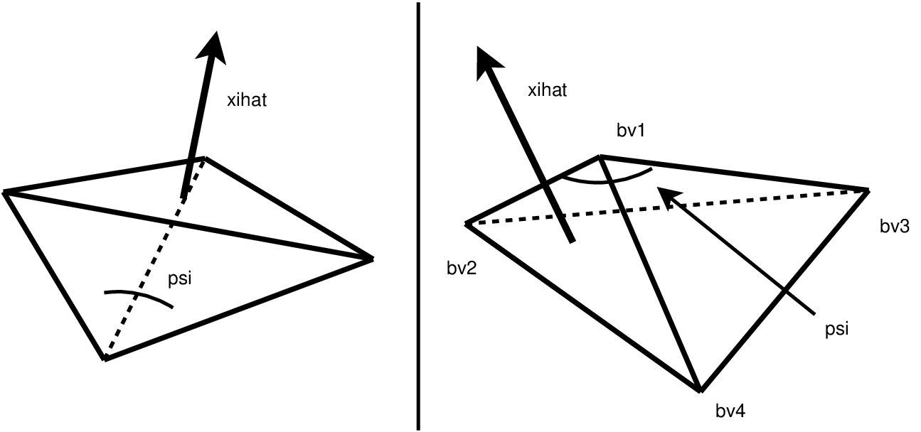
Construction is divided into two cases. First we suppose that is realized by a dihedral angle of the tetrahedron. Considering this largest dihedral angle, all vertices of the tetrahedron are contained in two planes that meet at angles of and . Selecting a vector that points “away” from these planes demonstrates
| (31) |
Next we suppose that is realized by an angle in one of the faces of the tetrahedron. Let be the vertex at which the angle occurs, let and denote the other two vertices of that triangle and let denote the last vertex; see Fig. 10. Moreover, without loss of generality we can assume that , i.e., is nearer to than . Let be the unit normal vector to the triangle with vertices , and . To bound , first observe that is orthogonal to three of the six lines containing edges of the tetrahedron. Two other edges belong to the triangle with vertices , , , i.e., the triangle with a largest angle . This large angle ensures that for any unit vector in the direction of either of these two lines, . Lastly, we consider unit vectors in the direction of the line through and . The triangle inequality implies
where the second term in the sum is zero by construction of orthogonal to the a plane containing and . Recalling our earlier argument, . Thus we can estimate the angle between and the line containing and .
| (32) |
The final inequality above follows from our definition of : . We thus conclude that
| (33) |
Considering the two expressions (31) and (33), we see that if is bounded away from , then is bounded away from .
Next we establish a reverse inequality. The crux of the argument is contained in an inequality from [2]. Defining , Acosta et al. assert that there are unit vectors , , in the directions of the edges of the tetrahedron such that
| (34) |
Letting be an arbitrary unit vector, we consider the decomposition where is a unit vector in the plane spanned by and . Since these are orthgonal subspaces, and thus or . If , then
| (35) |
Otherwise . Letting denote the non-acute angle between the lines containing and , we observe that (34) implies that or . Also the angle between and the line in the direction of either or is no larger than . Thus,
| (36) |
Despite the complex form, this is the desired inequality. Specifically, if is bounded away from , then is bounded away from zero. Since all the functions we consider are continuous, it follows that the argument of is also bounded away from zero. Thus is bounded away from . ∎
Appendix B Mollification
Proofs of several propositions in Section 2.1 are provided here.
Proof.
(Proposition 2.1) Define by and let be an arbitrary function. If then
The final equality results from the fundamental theorem of calculus. In the support of mollifier , so . Then Hölder’s inequality can be applied:
By selecting , the left-hand side of the above estimate becomes . Since , . Dividing both sides by gives the desired inequality. Density of smooth functions in is used to extend this result to the full space. ∎
Proof.
(Proposition 2.2) Let where is the characteristic function of . Applying Young’s inequality to gives
Since on , . Then recognizing that and computing the norm of yields the desired estimate. ∎