State Amplification Subject To Masking Constraints
Abstract
This paper considers a state dependent broadcast channel with one transmitter, Alice, and two receivers, Bob and Eve. The problem is to effectively convey (“amplify”) the channel state sequence to Bob while “masking” it from Eve. The extent to which the state sequence cannot be masked from Eve is referred to as leakage. This can be viewed as a secrecy problem, where we desire that the channel state itself be minimally leaked to Eve while being communicated to Bob. The paper is aimed at characterizing the trade-off region between amplification and leakage rates for such a system. An achievable coding scheme is presented, wherein the transmitter transmits a partial state information over the channel to facilitate the amplification process. For the case when Bob observes a stronger signal than Eve, the achievable coding scheme is enhanced with secure refinement. Outer bounds on the trade-off region are also derived, and used in characterizing some special case results. In particular, the optimal amplification-leakage rate difference, called as differential amplification capacity, is characterized for the reversely degraded discrete memoryless channel, the degraded binary, and the degraded Gaussian channels. In addition, for the degraded Gaussian model, the extremal corner points of the trade-off region are characterized, and the gap between the outer bound and achievable rate-regions is shown to be less than half a bit for a wide set of channel parameters.
I Introduction
I-A Problem Statement
In this paper, we consider a state dependent broadcast channel model with two users, and investigate the question of to what extent the state of the channel can be amplified at the receiver (Bob) and masked from the other receiver (referred to as Eve). The entire channel state sequence is presumed to be known non-causally to the transmitter (Alice). The only manner to affect the state information at Bob and Eve is by the encoding scheme used at the transmitter. For such a system, we aim to characterize the trade-off between the “amplification”-rate (at which the legitimate pair can operate) and the “leakage”-rate (to the eavesdropper).
Formally, consider a discrete memoryless channel given by , where is the channel input, is the channel state, and is the channel output. Here, corresponds to the received channel output at the legitimate receiver (Bob) and is the output at the eavesdropper (Eve). The channel is memoryless in the sense that
and the state sequence is independent and identically distributed (i.i.d.) according to a probability distribution indicated by . It is assumed that the channel state sequence is non-causally known at the transmitter. The system model is given in Fig 1.

The task of the encoder is to “amplify” the state sequence at Bob (channel output ) and to “mask” the state sequence from Eve (). Formally, the encoder is a mapping of channel state to the channel input , i.e., , which can be characterized by a conditional probability distribution . is said to be achievable, if for any given , there exist a sequence of encoders such that
| (1) |
| (2) |
for sufficiently large , where the mutual information terms are with respect to the joint distribution . The problem is to characterize all achievable (,) pairs, which we denote by the trade-off region .
The performance of the encoder is also quantified by measuring the difference between the achievable amplification and leakage rates. The differential amplification rate is said to be achievable if for some . The maximum value of the differential amplification rate is called as the differential amplification capacity, denoted by , where
Note that this quantity is a property of a given trade-off region and can play a role for some applications, as this difference measures the knowledge difference between the two receivers regarding the state of the channel. (This quantity, , is discussed further in the later parts of the sequel.) In general, we are not only interested in the knowledge difference, but also in the entire rate trade-off region, which constitutes the main focus of this paper.
A cost constraint may also be imposed on the channel input with
| (3) |
where defines the cost per input letter and the expectation is over the distribution of the channel input. In this scenario, we say is achievable under the cost function and at expected cost , if there exists a sequence of encoders satisfying (1), (2), and (3) in the limit of large . (We use this constraint for the Gaussian channel, where the cost is the average transmitted power.)
Finally, we note that the equivocation rate (denoted by ) can be used in this formulation as well. In particular, is said to be achievable, if there exists a sequence of encoders satisfying
for sufficiently large . Accordingly, the achievable pairs can be defined. Hence, the problem can be re-formulated in terms of equivocation rate, where we seek to characterize all achievable pairs in the limit of large . Since both the equivocation and leakage rate notions characterize the same trade-off, both notions can be used interchangeably.
I-B Related works and applications
The problem of communication over state dependent channels is studied by Gel’fand and Pinsker [1], where a message has to be reliably transmitted over the channel with non-causal state knowledge at the transmitter. The Gaussian version of the problem is solved in [2] through the famous dirty paper coding scheme. While the wiretap channel is introduced and solved in [3], these results are extended to a broadcast setting in [4]. The problem of sending secure messages over state dependent wiretap channels is studied in [5, 6].
On the other hand, the problems of state amplification and state masking are individually solved in [7, 8, 9] for point-to-point channels. Both [7, 8] and [9] consider the problem of reliable transmission of messages in addition to state amplification and state masking, respectively. In this paper, we consider the problem of amplifying the state to a desired receiver while trying to minimize the leakage to (or mask the state from) the eavesdropper. We note that, if we set in our problem definition, it reduces to the state masking problem as studied in [9]. In other words,
can be shown to be achievable [9]. Also, when , the problem reduces to a state amplification problem [8], and one can achieve the following rate pair.
These represent two extremes of the trade-off region between the amplification and masking rates. The main focus of this paper is to characterize the entire trade-off region of amplification and leakage rates. In the following, we list some applications of the proposed model.
I-B1 Broadcast channels
Communication over state dependent channels have a wide set of applications in broadcast channels, especially for the MIMO systems [10, 11, 12]. In such multi-user channels, an information-carrying signal can be modeled as a state sequence for another. As the transmitter knows the information-carrying signal for the first user, it can be treated as a known state for the transmission to the second user. In addition, the second signal (intended for the second user) can be considered as an overlay to the first one, especially for multicasting scenarios. (Here, the codeword of the first signal may follow an i.i.d. process, or this can be an uncoded information [9].) In such multi-user settings, the security of the communication arise as an important problem due to the broadcast nature of the medium. Utilizing the framework given in this paper, the amplification and leakage of the signals can be analyzed.
I-B2 Cognitive radio and relay channels
Another relevant setting where our results will be of significant interest is cognitive radio systems [13, 14, 15, 16, 17, 18, 19, 20]. For example, in an overlay conginitive radio scenario [16], the cognitive encoder (Alice) can facilitate the secure communication of the primary signal (the state sequence of the channel) by amplifying the signal at the primary receiver (Bob) while masking it from the eavesdropper (Eve). In such an application, the codebook information of the primary signal may be absent at the cognitive radio, and the formulation we have in this paper would be relevant. More generally, this setting belongs to user cooperation or relaying architectures that can increase the security of the communication systems [21, 22, 23, 24]. In an another cognitive radio setup, two cognitive users (Alice and Bob) can utilize the primary signal (interfering sequence ) to share a secret key between each other in the presence of an eavesdropper. (Applications to key sharing from channel states are detailed in the following.)
I-B3 Secret key generation from channel states
In recent years, a bridge between cryptography and information theoretic security has emerged in the form of channel state-dependent key generation [25, 26, 27, 28]. In this line of work, a state dependent channel (such as the wireless channel) is considered, and a function of this state is intended to be a “shared secret” between the legitimate transmitter (Alice) and legitimate receiver (Bob) while aiming to keep the eavesdropper (Eve) as much in the dark as possible. In the best case, the state(s) seen by Bob and Eve will be completely different (independent). However, the states of the channels are usually dependent. Moreover, for some models (e.g., the dirty paper coding setup [2]), there is a single channel state defining the channel for both Bob and Eve. (For example, at Bob and at Eve as considered in [29]. See also the discussion above for cognitive radio channels.) For such scenarios, as long as there is a non-trivial difference between the amplification and leakage rates, the state knowledge can be used to develop shared keys and enable cryptographic algorithms. For instance, utilizing the coding schemes proposed here, Bob can have bits of information regarding the channel state, where at most number of these bits are leaked to Eve. Then, privacy amplification [30] can be utilized to distill secret keys. That is, the methods provided in this paper can be utilized for the “advantage distillation” phase of a key agreement protocol [30]. In this form, the problem at hand is very much related to the generation of secrecy using sources and channels. Here, not only the source in the model is the channel state (different from the models studied in [31, 32]), but also it is non-trivially combined with the encoded signals of Alice (via the state dependent channel) to produce the observations at Bob and Eve. Hence, our formulation can be closely associated with the problem of secret key agreement over state dependent channels [33, 29]. In such problems, one is interested in the design of coding strategies that allow an agreement of secure bits between the legitimate users utilizing the state dependent channel. For example, sending secure bits over the channel will increase the secret key rate [29, 5, 6]. On the other hand, the problem studied in this work, when specialized to the differential amplification measure, is an analysis of the channel state knowledge difference. This analysis is very much related to the question of how many secret bits can be extracted from a given channel state ([25, 26, 27, 28]). We intend to provide information-theoretic guarantees (achievable rates and upper bounds) to the extent to which such a shared secret can be realized for our system model 11 1 We note that differential amplification capacity is related to the secret key rate that can be achieved utilizing the corresponding channel state. For example, consider , , where and are uniform bits. Here, when the state is defined as , and when the state is taken as , implying that bit of secret key rate can be supported.. Once obtained, this shared secret can now be employed to seed numerous symmetric key cryptosystems [34, 35].
I-B4 Watermarking and channel estimation
Consider that a host image is utilized in a watermarking scenario, where the encoder modifies the image in order to amplify it at the receiver and mask it from receiver . This model is similar to channel estimation scenarios in wireless communications. For example, a pilot signal can be constructed at the transmitter such that it not only facilitates the fading gain estimation at the receiver but also hides the channel state from the eavesdroppers as much as possible. For instance, while communicating to a base station for channel state estimation, a mobile user may want to hide this information from the external nodes in order to establish privacy of her location.
I-C Summary of results and organization
In this paper, we aim at developing an understanding of the trade-off between amplification and masking rates in a state dependent broadcast channel through achievable regions and outer bounds, and characterizing special cases when they match. The main results of this paper can be summarized as follows.
I-C1 Achievable Regions
The main achievability argument of the paper utilizes the transmission of a state dependent message over the state dependent channel. To facilitate this, we construct a (Gel’fand-Pinsker) codebook, wherein the corresponding codeword (denoted by ) carry this refinement information in such a way that reliable communication can be achieved over the state-dependent channel. Subsequently, we utilize this refinement information within a Wyner-Ziv coding scheme to derive expressions for the achievable amplification rates. In particular, we show that, even though the side information is not generated in an i.i.d. fashion, Wyner-Ziv approach can be used to facilitate amplification process. The leakage rates are then determined by deriving single-letter bounds on , and the achievable regions are established over the input probability distributions . The bounds show that the rate of the refinement message not only increases the amplification rate , but also increases the leakage rate , thereby establishing a trade-off for implementation.
I-C2 Secure Refinement
We show that it is possible to extend the proposed region by transmitting secure refinement information when Bob observes a “stronger” channel than Eve. In precise terms, this corresponds to instances of satisfying . Note that a channel is said to have a less noisy structure if for all input probability distributions [36, 37]. We find that the utilization of the notion of secure refinement approach is critical to such channels, and we show that the leakage due to transmission of the message can be minimized by securing the message. In the process of establishing these results, we also develop an alternate proof of secure message transmission over state dependent wiretap channels.
I-C3 Special Classes of Channels
Our outer bound arguments are based on upper bounding and lower bounding . The achievable schemes and outer bounds presented are used to establish optimality results for a class of channels. In particular, we show that the proposed scheme achieves the optimal differential amplification capacity (i.e., the maximum value of over the set of achievable pairs) for the reversely degraded discrete memoryless channel (DMC), the degraded binary channel, and the degraded Gaussian channel.
I-C4 Gaussian Channels
We characterize the corner points of the region for the degraded Gaussian channel. In this scenario, we further bound the gap between achievable and converse regions, and show the following: Let us denote the message capacity of Bob’s channel as and that of Eve’s channel as , where () is the signal-to-noise ratio of Bob (respectively, Eve). Then, for any given leakage rate , we show that the gap between the upper and lower bounds on the amplification rate is bounded by . Similarly, for any given amplification rate , we show that the achievable leakage rate is within of the lower bound on . In particular, the corresponding gaps are within half a bit when and , respectively.
The rest of the paper is organized as follows. Section II details the proposed coding schemes and presents the corresponding achievable regions. Section III provides the outer bounds to the trade-off region. Section IV includes optimality discussions and numerical results for special classes of DMCs including the reversely degraded channel, modulo additive binary channel model, and the memory with defective cells model. The Gaussian channel model is considered in Section V along with corresponding optimality results. Finally, we conclude the paper in Section VI. Some of the proofs are collected in appendices to improve the flow of the paper.
II Achievable Regions
We consider transmitting state dependent information over the state dependent channel. This refinement information can be utilized at Bob in resolving some ambiguity regarding the channel state. We divide the discussion into two parts, each providing a different scheme for the transmission of this refinement information.
II-A State enhanced messaging: Refinement
In order to facilitate the transmission of information regarding the state sequence, we consider an encoder that transmits a state dependent message over the state dependent channel. Here, by employing the Gel’fand-Pinsker coding [1], a rate of can be reliably communicated over the state dependent channel. Utilizing this communication rate, Alice can provide a refinement information to Bob. In particular, we consider a Wyner-Ziv coding [38] approach to provide such a refinement information (as discussed in [8]). Here, the side information at the receiver is - consisting of Gel’fand-Pinsker codeword and the observed sequence from the channel . For this side information scenario, we utilize the Gel’fand-Pinsker information rate as the bin index of a covering codeword . We note that, in the original setup of source coding with side information (aka Wyner-Ziv model), the side information is generated i.i.d. with the source sequence. For the scenario considered here, the side information is not in this form. In the following, we show that this issue can be resolved, and the Wyner-Ziv coding scheme can be utilized to increase the amplification rate. On the other hand, this transmission scheme may leak some state information to Eve. Accordingly, we obtain appropriate bounds on the leakage rate that depends on the Gel’fand-Pisker coding rate used for the refinement. The corresponding achievable region is given by the following.
Theorem 1
[Refinement] Let be the closure of the union of all pairs satisfying
over all distributions satisfying . Then, .
II-A1 Proof of Theorem 1
We provide main steps of the coding argument here and relegate some of the details to appendices.
Codebook Generation: Fix a and a . (The requirement on these distributions will be specified later.) Randomly and independently generate sequences , , each according to . Partition indices into equal-size subsets referred to as bins , . (This is the codebook used for Wyner-Ziv coding [38, 39].) For each , generate number of sequences randomly and independently according to . Index these sequences as with . (This is the codebook used for Gel’fand-Pinsker coding [1, 39].)
Encoding: Here, the encoder sets and and transmits message of rate with Gel’fand-Pinsker coding in order to perform refinement via Wyner-Ziv coding. Given , the encoder finds an index such that . If there exists more than one index, it selects one uniformly random among these. If there exists no such index, it selects one uniformly random from . From , encoder determines the bin index in the codebook such that . Then, it sets and finds an index such that . If no such (covering) index exists or if there are more than one, the encoder picks one uniformly at random. The encoder then transmits that is generated i.i.d. according to .
Amplification rate analysis: In the following, we show that the decoder can obtain codeword using Gel’fand-Pinsker decoding and then codeword by utilizing the side information . (This is the discussion provided in [8] for a state amplification mechanism, which we detail here.) We then provide a derivation of the state amplification rate utilizing this decoding mechanism.
Let . Upon receiving , decoder declares that and are chosen at the encoder, if these are the unique indices such that , otherwise it declares an error. (We remark that compared to the Gel’fand-Pinsker setup [1, 39], where only the message has to be uniquely decoded, we require decoder to obtain the codeword chosen at the encoder. This will be utilized in decoding error analysis.) Then, the decoder finds the unique index such that . Otherwise, it declares an error.
Consider the error event , where are the indices chosen at the transmitter, and are the indices decoded at the receiver. Decoder makes an error only if one or more of the following events occur.
Here, . By the union of events bound, we have
We bound each term above in the following.
a) By covering lemma [39], as , if
| (4) |
b) implies that , which implies that due to i.i.d. generation of from and the conditional typicality lemma [39] for some . Similarly, as is generated i.i.d. from through , we have as for some , again due to the conditional typicality lemma [39].
c) Each for some is distributed i.i.d. and independent of . By packing lemma [39], we have as , if
| (5) |
The three error analyses above are the same arguments used for decoding the message index in Gel’fand-Pinsker coding [1, 39].
d) The analysis for showing that as is detailed in Appendix A. We use the arguments given in [40] in order to show this. The original problem studied in [40] does not involve a state-dependent channel, but the coding scheme constructs channel inputs via , which can be viewed as a state dependent channel. (The argument we have here - the Gel’fand-Pinsker codeword decoded at the decoder is the same as the one chosen at the encoder - also appears in [41], which states that this observation follows from the arguments in [40, 42].)
e) By covering lemma [39], as , if
| (6) |
f) For analyzing , we note that one may not utilize conditional typicality lemma as done in the proof of Wyner-Ziv coding (see, e.g., [39, Section 11.3.1]). Because, the side information here, , is not generated i.i.d. through . Therefore, one can not go from joint typicality of to the joint typicality of . Instead, we consider the following approach: implies that
| (7) |
and implies that . Now, consider a pair . In addition, we have such that the pmf satisfies the following two conditions: The first condition is that
| (8) |
which is due to the fact that probability of the event vanishes. And, the second condition is that, for every and for sufficiently large ,
| (9) |
for some as . This second assertion, i.e., (9), follows from [39, Lemma 12.3]. Now, from (7), (8), (9), and the fact that forms a Markov chain, we obtain from Markov lemma [39] that, for some , . Denoting , the analysis above implies that as . (We note that, an analysis similar to the one above is given for the Berger-Tung inner bound in [39]. The difference here is that the bin index of the covering codeword determines the index of . Still, given a realization of , and hence , we have covering sequences, i.e., the set , for , from which the argument follows.) Then, by conditional typicality lemma [39], for some , we have , as (due to having w.h.p.), and . This implies that as .
g) Finally, analysis follows as that for the proof of Wyner-Ziv coding (see, e.g., [39, Section 11.3.1]). In particular, considering the event , [39, Lemma 11.1] shows that . Then, as each with is generated by and independent of , from packing lemma [39], as , if
| (10) |
Therefore, as , if (10) holds.
The analysis above implies that as if (4), (5), (6), and (10) hold. Here, we set and and , for some arbitrarily small and . This will satisfy (4) and (6). Furthermore, we set , which is the rate required to describe to the decoder. This will satisfy (10). Finally, for a given , we choose some to support transmission of the refinement message with rate . This will satisfy (5), as . We note that, as in above. Therefore, for a given , the proposed coding scheme supports any state refinement rate satisfying
Utilizing the analysis above, we now detail the derivation of the amplification rate. We start by defining an event indicator random variable . Consider setting , if a decoding error () occurs or the state sequence observed at the encoder () turns out to be non-typical. Set , otherwise. We continue with the following set of relations. (We drop the indicies of codewords.)
where (a) follows by the indicator event conditioning lemma given in Appendix B, (b) follows as , (c) is due to the definition of , wherein implies that , i.e., the decodability of the codewords form , (d) is by for some arbitrarily small as implies that is typical (and is generated i.i.d. here), (e) is by taking , which can be made arbitrarily small as (as as ), and lower bounding , which follows as implies that is typical (and is generated i.i.d. here), (f) follows as , and (g) is by . (This follows, as we set in the coding scheme.) From the last expression, we identify that any is achievable.
Leakage rate analysis: We first show the achievability of with the following.
where (a) follows as due to the fact that conditioning does not increase the entropy and as forms a Markov chain (this is due to i.i.d. generation of from , and i.i.d. generation of from ), and (b) follows as . (We note that single letterization argument for above is also given in (26) of [9].)
Next, we focus on the achievability of . We have the following.
where (a) is by adding as can be determined from for a given codebook, (b) follows as , (c) is due to having (a random variable with values has entropy at most ), (here, given , there are number of codewords, and the entropy of this set is maximized if the index has the uniform distribution), , and having , where the second inequality holds as forms a Markov chain (as detailed in the previous paragraph). (We note that single letterization arguments for and above are also given in (24) and (26) of [9].)
This concludes the proof of Theorem 1, where we take the union of the achievable pairs over all distributions.
II-A2 Message transmission
We note that it is possible to allocate a part of the Gel’fand-Pinsker coding rate in the scheme proposed above in order to transmit messages. In particular, if satisfies the inequalities given in Theorem 1, then is achievable with a message rate of . That is, the Gel’fand-Pinsker coding rate given by can be divided into refinement rate and message rate .
II-A3 State sequence covering
In the region given by Theorem 1, increasing will not only increase the amplification rate but will also increase the leakage rate. Therefore, for some scenarios, implementing only a covering scheme might be advantageous. By choosing an arbitrarily small refinement rate in Theorem 1, the following region can be achieved.
Corollary 2
[Covering] Let be the closure of the union of all pairs satisfying
over all distributions satisfying . Then, .
We note that the rate of refinement, , is set to an arbitrarily small value here, and the codeword only serves as a covering of the state sequence. Further implications of this covering scheme on the amplification-leakage region is discussed in Section IV-A. We note that, by transmission of a covering of the state, the leakage rate is shown to satisfy . Remarkably, one can guarantee such a bound, even if some state dependent information is transmitted over the channel. In particular, if the channel seen by Bob is stronger than the one seen by Eve, one can send the refinement information securely over the state dependent channel. This approach is detailed in the next section.
II-B Secure refinement
Consider all input distributions satisfying . For such distributions, it is possible to send refinement information securely over the channel. This way, the leakage increase due to refinement index is decreased as the security of the index will lower the corresponding leakage rate achieved at Eve compared to the non-secured case. In the following, we first focus on transmission of secure messages over the state dependent channel, and then detail the proposed secure refinement approach.
II-B1 Secure message transmission over state dependent channels
Consider that a transmitter wants to send a secure message over the state dependent channel in the presence of eavesdropper. This problem is studied in [5], and, we will revisit it here. In particular, we give a codebook construction and provide a lemma that upper bounds , the leakage to the eavesdropper 22 2 The codebook we provide here is a special case of the one proposed in [5], which considers an extended version for an equivocation rate analysis.. This result is then utilized in the following part, in showing the proposed secure refinement approach.
Codebook Generation: We divide the codebook construction in two parts, depending on whether or not. If , generate codewords , where , , and . Here, is randomly selected. We set and , which imply . If , generate codewords , where , . We set and . In both cases, is the secure message index, and is used as a covering index (similar to the previous section).
The above codebook construction is the same as that of Gel’fand-Pinsker codebook (described in the previous section), with the only difference being that, for probability distributions satisfying , we select a part of the message as random (represented as in the paragraph above). This enables to argue that the remaining part of the Gel’fand-Pinsker message (represented as in the paragraph above) is secure against the eavesdropper (in terms of the leakage rate). We have the following.
Lemma 3
For the codebook generation given above, for some as ,
where is a random variable uniformly distributed on the set for , and for .
Proof:
See Appendix C. ∎
This result is utilized in the next section for the secure refinement approach. Here, we note the following corollary, which is an alternate proof of security in state dependent wiretap channels.
Corollary 4
For the codebook generation given above, if is independent of , then
for some as .
Proof:
See Appendix D. ∎
II-B2 Secure refinement via secure and state dependent message transmission
In the previous section, a refinement approach is proposed where a Gel’fand-Pinsker coded message is utilized to resolve some ambiguity regarding the channel state at Bob. In such an approach, the message rate is utilized as the bin index of a covering () codebook. (See proof of Theorem 1.) Here, we consider transmission of this refinement message securely to Bob by utilizing the codebook construction given above. As the message rate is modified from to secure message rate , this modification results in a refinement rate of . However, the leakage rate due refinement is now independent of . The corresponding region is given by the following.
Theorem 5
Let be the closure of the union of all pairs satisfying
over all distributions satisfying Then, .
Note that, the amplification rate that can be obtained with such an approach is lower than the previous case (Theorem 1), as the message rate if . Therefore, the improvement on the leakage expression compared to Theorem 1 is obtained with a degradation on the amplification rate.
Proof:
We use the codebook generation given above. The only difference compared to the codebook construction utilized in the proof of Theorem 1 is that part of the message (i.e., ) is selected as random when . Therefore, the amplification rate analysis is the same as that of the one given in the proof of Theorem 1 with bounded by instead of . The proof of follows from the same steps given in the proof of Theorem 1. Here, we show that holds as well.
Consider the following.
where (a) follows from Lemma 3, (b) follows as and , and (c) follows by observing , where for ; and, is independently generated random variable for , implying that . As can be made arbitrarily small, we conclude from last expression that any is achievable. ∎
III Outer Bounds
In this section, we provide outer bounds on the achievable amplification-leakage rate region. In particular, we derive regions denoted by , to which any achievable must belong.
Proposition 6
If is achievable, then , where is the closure of the union of all pairs satisfying
over all distributions satisfying .
Proof:
See Appendix E. ∎
If the channel is degraded, wherein , the following outer bound can be obtained.
Proposition 7
If the channel satisfies and if is achievable, then , where is the closure of the union of all pairs sarisfying
over all distributions satisfying .
Proof:
See Appendix F. ∎These outer bound regions are used in the following to establish special case results.
IV Special discrete memoryless channel models
IV-A Reversely degraded DMCs
We say that the channel is reversely degraded if forms a Markov Chain. Note that, this corresponds to a stronger channel seen by Eve compared to that of Bob. Therefore, reversely degraded scenarios imply , meaning that the state knowledge at Bob is not higher than that of at Eve. We have the following result for this set of channels.
Theorem 8
The optimal differential amplification rate for reversely degraded DMCs is given by
Proof:
Achievability of the stated difference follows from Theorem 1 by substituting . We provide the converse in Appendix G. ∎
Note that coding can not improve this difference as the channel is reversely degraded. Thus, coding might help to increase at the expense of possibly decreasing for the reversely degraded scenario. This is also the case for the covering scheme given by Corollary 2. That is, vs. can be traded-off using different input distributions. ( case will correspond to the maximum , and achieve .)
IV-B Modulo additive binary model
Consider the channels given by
where the state and noise distributions are generated i.i.d. as , , . (All s satisfy for .) In this section, we use the following notation for the binary convolution .
IV-B1 State cancellation scheme
To cancel the state from the channel, we send
where and the codewords carry a description of the state sequence . This way, we achieve the following inner-bound.
Corollary 9
The state cancellation scheme, which sends distributed signal XORed with state sequence at each time instant, achieves the set of pairs denoted by the region , where
with
Proof:
Achievability follows from Corollary 2. ∎
IV-B2 Optimal differential amplification rate
Corollary 10
If and for a binary model, the optimal amplification and leakage rate difference is given by
Proof:
From Proposition 7, we obtain the following. If , any given satisfies
Note that, this upper-bound can be evaluated by observing
where the equality is due to the channel degradedness condition with appropriate noise term independent of such that , and the inequality is due to the fact that conditioning does not increase the entropy. Using this we observe that the outer-bound is maximized with a choice of , which evaluates to
This expression is achieved by Corollary 9, when we choose , if . ∎
IV-C Memory with defective cells model
We consider the model of information transmission over write-once memory device with stuck-at defective cells [43, 44, 45]. In this channel model, each memory cell corresponds to a channel state instant with cardinality , where the binary channel output is determined from the binary channel input and the channel state as:
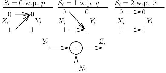
where is the probability that the channel is stuck at , is the probability that the channel is stuck at , and is the probability of having a good channel where with . We consider a binary symmetric channel (BSC) from to , where
with for some . This corresponds to a degraded DMC model. (See Fig. 2.)
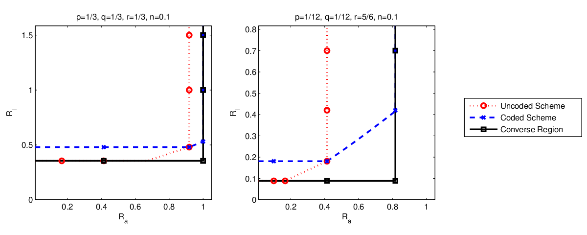
We present numerical results for this channel model with three regions: Uncoded region, coded region, and an outer-bound region. The uncoded region is obtained by setting in Theorem 1, where we have the set of pairs satisfying
over all possible . For the coded region, we simulate a sub-region of the one given in Theorem 1, where we set and achieve the set of pairs satisfying
over all possible . For converse arguments, we consider the outer-bound region given by the set of pairs satisfying
over all possible . This outer-bound region follows from Proposition 6. We evaluate the regions above in terms of the channel parameters as follows. Let . Then,
where is the ternary entropy function, is the binary entropy function, and is the binary convolution given by . The numerical results are given in Fig. 3. The regions are truncated with as any is trivially achievable. We note that, the coded region is potentially larger than its uncoded counterparts even when we only compute a subset of the coded achievable region. This shows the gains that can be leveraged by the proposed scheme, i.e., sending a refinement of the state sequence over the channel.
V Gaussian Scenario
Consider the channels given by
where the state and noise distributions are generated i.i.d. as , , , and the cost constraint on the channel input is given by and , i.e., (See Fig. 4.)

V-A An inner bound for using an uncoded scheme
The inner bound is based on sending an amplified version of together with some additional Gaussian noise. This uncoded signal is constructed as follows.
| (11) |
where independent of , , and . Here, is the fraction of the power allocated to . This scheme achieves the following region.
Theorem 11
The uncoded scheme, which forwards at each time step together with some i.i.d. Gaussian noise as given in (11), achieves the set of pairs denoted by the region , where
with
| (12) | |||||
| (13) |
The expressions above are obtained by evaluating and on account of uncoded transmission in (11).
Examples:
- •
If , one can set and achieve the pair
- •
Another trivial point is obtained by setting , which achieves
V-B Outer-bounds on
Corollary 12
Let denote the correlation coefficient between and . The set of all achievable rate pairs , satisfy
for and .
Proof:
Using Proposition 7, we have
| (14) |
Using Proposition 7, the linear estimate , and the fact the conditioning does not increase entropy, we get
Since the entropy maximizing distribution for a given second moment is a Gaussian, we have
leading to
∎
Corollary 13
Let denote the correlation coefficient between and . If , then the set of all achievable rate pairs satisfy
| (15) |
for and .
Proof:
By Proposition 7, we have
Without loss of generality, we consider with where is independent of . Noting that,
we upper bound using the following. Consider two zero-mean correlated random variables and .
where in (a) we used as the estimate of given , and (b) follows by defining the estimation error variance and the fact that Gaussian distribution maximizes entropy given the variance. We then upper bound the optimal estimator error variance by the linear MMSE variance. Therefore,
Using the above, we obtain
| (16) | |||||
This completes the proof. ∎
V-C Comparison of inner and outer bounds for the degraded Gaussian channel
We now compare the uncoded scheme and the outer bound presented above. In particular, we show that the uncoded transmission scheme achieves certain corner points of the amplification-masking region and that the gap between the inner and outer bounds on the region is within bits for a wide set of channel parameters. We also show that the uncoded scheme achieves the optimal difference .
V-C1 Characterization of the gap between achievable and converse regions
We show that given any point in the converse region corresponding to a given , uncoded transmission achieves within bits of the converse region under certain conditions on channel parameters. In particular, for any given , uncoded transmission achieves that and within bits of the bound on if . Similarly for any given , uncoded transmission achieves the given and within bits of the bound on if . We prove these as follows. Using Corollary 12, any point in the outer bound region is described as
| (17) |
for and . Now let us show that uncoded transmission achieves any in the region above and the gap from as above is within bits. Let the uncoded scheme be designed such that , where and independent of . Now, by (13) and (12) this input achieves a leakage, and given by , which implies that the gap is given by
| (18) |
for . Now, in order to prove the other claim, that uncoded achieves any given and the gap with is within bits, we proceed as follows. Given , we achieve this by choosing an uncoded scheme such that if or if . We choose such that
where . By the intermediate value theorem for continuous functions, it is clear that there exists such that the conditions above are satisfied. Further, the uncoded scheme achieves the desired . For , the scheme achieves an given by leading to a gap
| (19) |
when . Following the same steps, case can be shown as well, implying the characterization of the trade-off region within bits for and .
V-C2 Differential amplification capacity
V-C3 Corner points of the trade-off region
Consider the corner points of the amplification-masking region. Inspecting (12), we observe that the point in the outer bound region corresponding to maximum amplification is given by . Clearly, from (18) and (19), we see that the gap is zero for . Similarly, consider the point corresponding to minimum leakage in the weak and moderate interference regimes as in [9]. These points correspond to and we have and , leading to the gap being zero. This is also verified by setting in (18) and (19).
V-C4 Numerical results
We compare the uncoded region with an outer-bound region (given in Proposition 12) in Fig. 5. The first case corresponds to a degraded scenario, where the gap between the regions is fairly small as expected from the analysis given above. However, for the reversely degraded scenario with larger power constraint compared to the state power , the gap is larger. In Fig. 6, we plot the differential amplification capacity for a degraded channel (, ) for a range of power constraints and different values of . Note that the differential amplification capacity saturates in the high SNR regime, and the effect of encoder in increasing is decreasing as the power of the additive state increases.


VI Conclusion
We study the problem of state amplification under the masking constraints, where the encoder (with the knowledge of non-causal state ) facilitates the amplification rate () at Bob, which observes , while minimizing the leakage rate () as much as possible at Eve, which observes . Our coding schemes are based on transmission of state dependent messages over the state dependent channel to Bob. The achievable region corresponding to this refinement strategy is derived by calculating bounds on amplification and masking rates. We also show that for the input distributions enabling Bob to be a “stronger” receiver than Eve, the refinement information can be sent securely over the channel. This secure refinement approach is shown to lead to non-trivial achievable regions. We also provided outer bounds, using which we showed that the scheme without secure refinement achieves the optimal over the region in the reversely degraded DMCs, the degraded binary channels, and Gaussian channels. For the degraded Gaussian model, we also characterized the optimal corner points, and the gap between the outer bound and achievable regions.
Several interesting problems can be considered as future directions. First, the channel cost may be introduced for the DMC model as well, and the cost may have some dependence on the state sequence or vary according to a stochastic model. Second, causal channel state knowledge can be considered. Third, in addition to the task of state amplification and masking, transmission of messages to the receivers can be considered. Towards this end, signaling techniques for (secure) broadcast channel models can be utilized. Another extension direction is the coded state sequence setting [45], which is a scenario that is more relevant to the broadcast and cognitive radio systems, where the coded signal (that carries a message from a codebook) corresponds to the channel state sequence that is non-causally known at the encoder. Finally, a source coding extension of the current model can be studied. In such a problem setup, the trade-off between the distortions achieved at both users can be analyzed. A relevant work for such an extension is [46], where a source coding setup is considered with two sources (one has to be amplified and the other has to be masked) with a single receiver. We remark that the amplification and leakage rates analyzed in this paper can be utilized to provide a lower bound on the distortion that can be achieved at Bob and Eve, respectively, by evaluating the corresponding distortion-rate functions.
acknowledgement
The authors are thankful to Yanling Chen of Ruhr-University Bochum, Yeow-Khiang Chia of Institute for Infocomm Research, Vincent Y. F. Tan of National University of Singapore, and anonymous reviewers for their valuable feedback.
Appendix A as
We use the arguments given in [40] in order to show this. Similar to the joint source-channel coding scenario studied in [40], we have a codeword with a covering index , which makes the codebook and covering index dependent to each other. In other words, sequence realization together with the codebook determines the index , from which generates through an i.i.d. generation process. Under such a scenario, as reported in [40], decoding the index with at receiver is successful if the number of indices is less than . We now provide this analysis here for completeness. Using the steps given in [40] for the scenario here, we have the following: For a given , we have number of codewords (), and the bound below.
where (a) is due to the union of events bound, and (b) follows by the symmetry of the codebook generation and coding, (c) is by defining , (d) is due to the fact that given , forms a Markov chain, (e) is due to Lemma 14 given at the end of this section, (f) is due to Lemma 15 given at the end of this section, (g) is due to having i.i.d. generation for , i.e., , (h) is due to joint typicality lemma [39].
From the last expression, we obtain that as , if . This implies the existence of sequence of codes implying the desired result as we set .
Lemma 14 (Lemma 1 in [40])
For sufficiently large ,
Proof:
We have
where (a) is due to independence of and together with bounding , and (b) follows from , as shown below.
Consider . Then, if , by the symmetry of the codebook generation and coding,
where we upper bound the probability with and used . On the other hand, if , for sufficiently large , and due to the symmetry of the codebook generation and coding, we have
where bound the probability with and utilized the joint typicality lemma [39]. The last inequality holds in the limit of large as and , where as . ∎
Lemma 15 (Lemma 2 in [40])
For sufficiently large ,
Proof:
We have
where (a) follows as , and (b) is due to having for sufficiently large due to the symmetry of the codebook generation and coding. ∎
Appendix B Indicator event conditioning lemma
Lemma 16
Consider an indicator random variable , where for , and for , for an event . Then, for any ,
Appendix C Proof of Lemma 3
Proof:
We first consider case, for which the codewords are represented by .
where (a) follows by , for some as (this is decoding of at eavesdropper having , following from steps similar to the proof of Theorem 1 replacing Bob with Eve, as number of indices is , see also Appendix A), , and having as is a one-to-one function of , (b) follows by as is independent of and uniformly random and taking , (c) follows as and as uniquely determined given , (d) is by having H(Z^n—M,T,S^n,U^n)=∑_i=1^n H(Z_i—Z_1^i-1,M,T,S^n,U^n)=∑_i=1^n H(Z_i—S_i,U_i)=nH(Z—S,U), which is due to the Markov chain as generates which generates i.i.d. due to the memoryless channel.
Secondly, consider case, for which the codewords are represented by . We consider with and , which together represent the covering index . (This can be obtained via random binning of number of codewords , , into bins represented by , where the codeword index per bin represented by .) We continue as follows.
where (a) follows by having as described above, , for some as (this is decoding of at eavesdropper having , following from steps similar to the proof of Theorem 1 replacing Bob with Eve, as number of indices is , see also Appendix A), , having as is determined by , and defining , (b) is by , and (c) is same as that of the step (d) of the previous paragraph.
∎
Appendix D Proof of Corollary 4
From Lemma 3, we have
Here, . In addition, as is generated i.i.d., and also independent of , we have with some as . (The latter expression follows as we can bound where is an indicator random variable with if is typical. Then, for some arbitrarily small , from which the assertion follows by taking .) Then, using these two observations in the equation above, we obtain , which concludes the proof.
Appendix E Proof of Proposition 6
Proof:
Define a random variable uniform over and independent of everything else. (A standard technique of using as a time sharing parameter will be utilized in the following.) Also define . We have the following bounds.
| (21) |
where (a) is due to the memoryless channel and the fact that conditioning does not increase the entropy, (b) follows from the distribution of , (c) follows as the added term . In addition,
| (22) |
where (a) holds as has an i.i.d. distribution. Moreover,
| (23) |
where (a) is due the fact that conditioning does not increase the entropy, (b) follows from the definition of , and (c) is the standard time sharing argument. Finally, we have
| (24) |
where (a) follows by Csiszár’s sum lemma [39] (note that this is similar to the converse result of the Gel’fand-Pinsker problem given in [44], where the indices of and are reversed), (b) is due to as has an i.i.d. distribution, (c) follows from definition of , (d) is the standard time sharing argument.
Now, define , independent of (note that this argument is also used in [9] in the corresponding single-letterization arguments), , , and . Then, (21) implies as due to the memoryless channel . (22) reduces to , as is independent of . (23) implies as due to the independence of and . (24) is . Consider adding to the right hand side of this inequality. We have, as and are independent, , and hence . Then, , which implies as a necessary condition.
This concludes the proof, as combining the bounds above with the fact that any achievable for the given channel and should satisfy and implies the inequalities stated in the proposition. ∎
Appendix F Proof of Proposition 7
Proof:
Let denote the set of satisfying , and denote denote the set of satisfying . For the channel , any also satisfies . Therefore, using the Proposition 6, we have that if is achievable, then , where
satisfying
It remains to show bound. We add the following bound to the ones stated above. (Note that, we use the same and -dependent definitions stated in Appendix E, and hence the following bound can be added to the ones stated in Appendix E.)
where (a) and (b) are due to the degradedness condition, (c) is due to the fact that conditioning does not increase entropy and the Markov chain as generates , (d) follows from the memoryless property of the channel, (d) and (f) are due to definitions given in Appendix E, (e) is by adding the non-negative term , and (g) is due to the Markov chain as outputs are generated i.i.d. using over the memoryless channel . The result then follows by taking the union over all joint distributions . ∎
Appendix G Proof of the converse for Theorem 8
Proof:
We bound the rate difference as follows.
where, in (a), we used the equalities
and
in (b), we used the Csiszar’s sum lemma [4] (and a conditional form of it) to obtain the equalities
and
in (c), we define ; and use the reversely degradedness of the channel resulting in , in (d), we obtain the single-letter expression (by defining , etc., see, e.g., [47]). Note that, with the definition of in (c), is generated from , and hence from . In addition, given , is independent of . Thus, forms a Markov chain, and the upper bound is given by
where the equalities follow due to the following: First, the conditional mutual information expression is maximized with a particular input (as randomizing over different values will not increase the sum ) and a probability distribution . Second, the optimal will correspond to a . Thus, the converse result can be stated over input distributions in the form , matching to the achievability result. ∎
References
- [1] S. Gel’fand and M. Pinsker, “Coding for channels with random parameters,” Probl. Contr. and Inform. Theory, vol. 9, no. 1, pp. 19–31, 1980.
- [2] M. H. M. Costa, “Writing on dirty paper,” IEEE Trans. Inf. Theory, vol. 29, no. 3, pp. 439–441, May 1983.
- [3] A. Wyner, “The wire-tap channel,” The Bell System Technical Journal, vol. 54, no. 8, pp. 1355–1387, Oct. 1975.
- [4] I. Csiszár and J. Körner, “Broadcast channels with confidential messages,” IEEE Trans. Inf. Theory, vol. 24, no. 3, pp. 339–348, May 1978.
- [5] Y. Chen and A. J. H. Vinck, “Wiretap channel with side information,” IEEE Trans. Inf. Theory, vol. 54, no. 1, pp. 395–402, Jan. 2008.
- [6] C. Mitrpant, A. J. H. Vinck, and Y. Luo, “An achievable region for the Gaussian wiretap channel with side information,” IEEE Trans. Inf. Theory, vol. 52, no. 5, pp. 2181–2190, May 2006.
- [7] A. Sutivong, M. Chiang, T. M. Cover, and Y.-H. Kim, “Channel capacity and state estimation for state-dependent Gaussian channels,” IEEE Trans. Inf. Theory, vol. 51, no. 4, pp. 1486–1495, Apr. 2005.
- [8] Y.-H. Kim, A. Sutivong, and T. M. Cover, “State amplification,” IEEE Trans. Inf. Theory, vol. 54, no. 5, pp. 1850–1859, May 2008.
- [9] N. Merhav and S. Shamai, “Information rates subject to state masking,” IEEE Trans. Inf. Theory, vol. 53, no. 6, pp. 2254–2261, Jun. 2007.
- [10] G. Caire and S. Shamai, “On the achievable throughput of a multiantenna Gaussian broadcast channel,” IEEE Trans. Inf. Theory, vol. 49, no. 7, pp. 1691–1706, July 2003.
- [11] G. Caire, S. Shamai (Shitz), Y. Steinberg, and H. Weingarten, “On information-theoretic aspects of MIMO broadcast channels,” in Space Time Wireless Systems, From Array Processing to MIMO Communications, H. B olcksei, D. Gesbert, C. B. Papadias, and A.-J. van der Veen, Eds. London, UK: Cambridge Univ. Press, 2008.
- [12] S. A. Jafar, G. J. Foschini, and A. J. Goldsmith, “PhantomNet: Exploring Optimal Multicellular Multiple Antenna Systems,” EURASIP Journal on Advances in Signal Processing, no. 5, pp. 591–605, May 2004.
- [13] J. Mitola III and G. Q. Maguire Jr., “Cognitive radio: Making software radios more personal,” IEEE Personal Commun. Mag., vol. 6, no. 4, pp. 13–18, Aug. 1999.
- [14] J. Mitola III, “Cognitive radio: An integrated agent architecture for software defined radio,” Ph.D. dissertation, Computer Communication System Laboratory, Department of Teleinformatics, Royal Institute of Technology (KTH), Stockholm, Sweden, May 2000.
- [15] N. Devroye, P. Mitran, and V. Tarokh, “Achievable rates in cognitive radio channels,” IEEE Trans. Inf. Theory, vol. 52, no. 5, pp. 1813–1827, May 2006.
- [16] A. Goldsmith, S. Jafar, I. Maric, and S. Srinivasa, “Breaking Spectrum Gridlock With Cognitive Radios: An Information Theoretic Perspective,” Proceedings of the IEEE, vol. 97, no. 5, pp. 894–914, May 2009.
- [17] Y. Liang, A. Somekh-Baruch, H. V. Poor, S. Shamai, and S. Verdu, “Capacity of cognitive interference channels with and without secrecy,” IEEE Trans. Inf. Theory, vol. 55, no. 2, pp. 604–619, Feb. 2009.
- [18] O. Simeone and A. Yener, “The cognitive multiple access wire-tap channel,” in Proc. 43rd Annual Conference on Information Sciences and Systems (CISS 2009), Baltimore, MD, Mar. 2009.
- [19] L. Toher, O. O. Koyluoglu, and H. E. Gamal, “Secrecy games over the cognitive channel,” in Proc. 2010 IEEE International Symposium on Information Theory (ISIT 2010), Austin, TX, Jun. 2010.
- [20] J. Zhang and M. Gursoy, “Secure relay beamforming over cognitive radio channels,” in Proc. 45th Annual Conference on Information Sciences and Systems (CISS 2011), Baltimore, MD, Mar. 2011.
- [21] L. Lai and H. El Gamal, “The relay-eavesdropper channel: Cooperation for secrecy,” IEEE Trans. Inf. Theory, vol. 54, no. 9, pp. 4005–4019, Sep. 2008.
- [22] R. Tandon, S. Ulukus, and K. Ramchandran, “Secure source coding with a helper,” in Proc. 47th Annual Allerton Conference on Communication, Control, and Computing (Allerton 2009), 2009.
- [23] O. O. Koyluoglu and H. El Gamal, “Cooperative encoding for secrecy in interference channels,” IEEE Trans. Inf. Theory, vol. 57, no. 9, pp. 5682–5694, Sep. 2011.
- [24] M. Yuksel, X. Liu, and E. Erkip, “A secure communication game with a relay helping the eavesdropper,” IEEE Trans. Inf. Forensics Security, vol. 6, no. 3, pp. 818–830, Sep. 2011.
- [25] B. Azimi-Sadjadi, A. Kiayias, A. Mercado, and B. Yener, “Robust key generation from signal envelopes in wireless networks,” in Proc. 14th ACM Conference on Computer and Communications Security (CCS 2007), Alexandria, VA, Oct. 2007.
- [26] S. Mathur, W. Trappe, N. Mandayam, C. Ye, and A. Reznik, “Radio-telepaty extracting a secret key from an unauthenticated wireless channel,” in Proc. 14th ACM International Conference on Mobile Computing and Networking (MobiCom 2008), San Francisco, CA, Sep. 2008.
- [27] S. Jana, S. N. Premnath, M. Clark, S. K. Kasera, N. Patwari, and S. V. Krishnamurthy, “On the effectiveness of secret key extraction from wireless signal strength in real environments,” in Proc. 15th Annual International Conference on Mobile Computing and Networking (MobiCom 2009), Beijing, China, Sep. 2009.
- [28] S. Mathur, A. Reznik, Y. Shah, W. Trappe, and N. B. Mandayam, “Information-theoretically secret key generation for fading wireless channels,” IEEE Trans. Inf. Forensics Security, vol. 5, no. 2, pp. 240–254, Jun. 2010.
- [29] A. Khisti, S. Diggavi, and G. Wornell, “Secret-key agreement with channel state information at the transmitter,” IEEE Trans. Inf. Forensics Security, vol. 6, no. 3, pp. 672 –681, Sep. 2011.
- [30] C. H. Bennett, G. Brassard, C. Crepeau, and U. M. Maurer, “Generalized privacy amplification,” IEEE Trans. Inf. Theory, vol. 41, no. 6, pp. 1915–1923, Nov. 1995.
- [31] A. Khisti, S. N. Diggavi, and G. Wornell, “Secret-key generation with correlated sources and noisy channels,” in Proc. 2008 IEEE International Symposium on Information Theory (ISIT’08), Jul. 2008.
- [32] V. Prabhakaran, K. Eswaran, and K. Ramchandran, “Secrecy via sources and channels: A secret key - secret message rate tradeoff region,” in Proc. 2008 IEEE International Symposium on Information Theory (ISIT’08), Jul. 2008.
- [33] A. Khisti, “Secret key agreement on wiretap channels with transmitter side information,” in Proc. 16th European Wireless Conference (EW 2010), Lucca, Italy, Apr. 2010.
- [34] H. Delfs and H. Knebl, Introduction to Cryptography: Principles and Applications, 2nd ed. Springer, 2007.
- [35] O. Goldreich, Foundations of Cryptography: Volume II, Basic Applications. Cambridge University Press, 2004.
- [36] J. Körner and K. Marton, “A source network problem involving the comparison of two channels II,” Trans. Colloquim Inform. Theory, Aug. 1975, Keszthely, Hungary.
- [37] ——, “Comparison of two noisy channels,” Topics in Information Theory, Coll. Math. Soc. J. Bolyai No. 16, Ed. P. Elias and I. Csiszár, North Holland, pp. 411–423, 1977.
- [38] A. Wyner and J. Ziv, “The rate-distortion function for source coding with side information at the decoder,” IEEE Trans. Inf. Theory, vol. 22, no. 1, pp. 1 – 10, Jan. 1976.
- [39] A. El Gamal and Y.-H. Kim, Network information theory. Cambridge University Press, 2011.
- [40] S. Lim, P. Minero, and Y.-H. Kim, “Lossy communication of correlated sources over multiple access channels,” in Proc. 48th Annual Allerton Conference on Communication, Control, and Computing (Allerton 2010), Allerton, IL, Sep. 2010.
- [41] C. Choudhuri and U. M. Ming, “On non-causal side information at the encoder,” in Proc. 50th Annual Allerton Conference on Communication, Control, and Computing (Allerton 2012), Monticello, IL, Oct. 2012.
- [42] A. Lapidoth and S. Tinguely, “Sending a bivariate Gaussian over a Gaussian MAC,” IEEE Trans. Inf. Theory, vol. 56, no. 6, pp. 2714–2752, Jun. 2010.
- [43] A. V. Kuznetsov and B. S. Tsybakov, “Coding in a memory with defective cells,” Probl. Peredachi Inf., vol. 10, no. 2, pp. 52–60, 1974.
- [44] C. Heegard, “Capacity and coding for computer memory with defects,” Ph.D. dissertation, Stanford University, Stanford, CA, Nov. 1981.
- [45] C. Heegard and A. E. Gamal, “On the capacity of computer memory with defects,” IEEE Trans. Inf. Theory, vol. 29, no. 5, pp. 731–739, Sep. 1983.
- [46] T. Courtade, “Information masking and amplification: The source coding setting,” in Proc. 2012 IEEE International Symposium on Information Theory (ISIT 2012), Cambridge, MA, Jul. 2012.
- [47] T. Cover and J. Thomas, Elements of Information Theory. John Wiley and Sons, Inc., 1991.