跳到论文正文
W Papers独立论文阅读器 arXiv:1112.3895 论文正文 计算阅读时间 · 0%
引用这篇论文根据当前论文元数据生成,正式投稿前建议核对。


License: arXiv.org perpetual non-exclusive license
arXiv:1112.3895v2 [astro-ph.CO] 22 May 2012

Constructing Regularized Cosmic Propagators

Francis Bernardeau Affiliation: Institut de Physique Théorique, CEA, IPhT, F-91191 Gif-sur-Yvette, France CNRS, URA 2306, F-91191 Gif-sur-Yvette, France    Martín Crocce Affiliation: Institut de Ciències de l’Espai, IEEC-CSIC, Campus UAB, Facultat de Ciències, Torre C5 par-2, Barcelona 08193, Spain    Román Scoccimarro Affiliation: Center for Cosmology and Particle Physics,
Department of Physics, New York University, New York, NY 10003
August 24, 2026
Abstract

We present a new scheme for the general computation of cosmic propagators that allow to interpolate between standard perturbative results at low-kk and their expected large-kk resummed behavior. This scheme is applicable to any multi-point propagator and allows the matching of perturbative low-kk calculations to any number of loops to their large-kk behavior, and can potentially be applied in case of non-standard cosmological scenarios such as those with non-Gaussian initial conditions. The validity of our proposal is checked against previous prescriptions and measurements in numerical simulations showing a remarkably good agreement. Such a generic prescription for multi-point propagators provides the necessary building blocks for the computation of polyspectra in the context of the so-called Γ\Gamma-expansion introduced by Bernardeau et al. (2008). As a concrete application we present a consistent calculation of the matter bispectrum at one-loop order.

I Introduction

The large-scale structure of the universe that we observe today is thought to emerge from gravitational instabilities out of primordial metric perturbations, therefore precise observations of the large-scale structure of the local universe can be used to put constraints on cosmological models. The connection between cosmological parameters and observations are however only straightforward when they correspond to the linear regime, i.e. when the observables can be computed as a linear transform of the primordial metric perturbations; this connection is less trivial when nonlinearities, due in a large part to the gravitational dynamics itself, are present. Those nonlinearities arise during the late stage of the gravitational instabilities. This is an epoch during which the universe can be safely assumed to be matter dominated (at least in the context of the standard model of cosmology where the dark energy component forms an homogeneous fluid.)

According to the cosmological principle cosmic fields are statically homogeneous and isotropic. In the context we are interested in, two degrees of freedom are then relevant (see [1] for details): the local density contrast, δ⁡(𝐱)\delta({\bf x}) and the velocity divergence, θ⁡(𝐱)=∂i𝐮i​(𝐱)\theta({\bf x})=\partial_{i}{\bf u}_{i}({\bf x}). It is then very fruitful to introduce the Fourier modes of the cosmic fields δ⁡(𝐤)\delta({\bf k}) and θ⁡(𝐤)\theta({\bf k}), which evolve independently of one another in the linear regime. One can then introduce the doublet Ψa(𝐤)={δ(𝐤),−θ(𝐤)/ℋ}\Psi_{a}({\bf k})=\left\{\delta({\bf k}),-\theta({\bf k})/{\cal H}\right\}, where ℋ{\cal H} is the conformal expansion rate with its time evolution described by the Friedmann equation, to write down the equations of motion in compact form and facilitate the implementation of resummation techniques.

In this context, the goal of the theoretical and numerical calculations is a precise description, beyond the linear regime, of the statistical properties of Ψa\Psi_{a}. We are particularly interested in the multi-component power spectra Pa​b​(k)P_{ab}(k) defined as,

⟨Ψa​(𝐤)​Ψb​(𝐤′)⟩=δD​(𝐤+𝐤′)​Pa​b​(k)\big<\Psi_{a}({\bf k})\Psi_{b}({\bf k}^{\prime})\big>=\delta_{\rm D}({\bf k}+{\bf k}^{\prime})P_{ab}(k) (1)

where the Latin indices aa and bb vary from 1 to 2, which are implicitly or explicitly measured in observations such as galaxy surveys, and higher-order spectra such as bispectra,

⟨Ψa​(𝐤1)​Ψb​(𝐤2)​Ψc​(𝐤3)⟩=δD​(𝐤1+𝐤2+𝐤3)​Ba​b​c​(𝐤1,𝐤2).\big<\Psi_{a}({\bf k}_{1})\Psi_{b}({\bf k}_{2})\Psi_{c}({\bf k}_{3})\big>=\delta_{\rm D}({\bf k}_{1}+{\bf k}_{2}+{\bf k}_{3})B_{abc}({\bf k}_{1},{\bf k}_{2}). (2)

This problem is in general very complicated if one wants to solve it from first principles. It can be made slightly easier to address in the context of the standard cosmological model where the primordial metric perturbations are expected to follow Gaussian or near Gaussian statistics. In that case the primordial properties of the fields are entirely determined by the initial power spectra, Pa​binit.​(k)P_{ab}^{{\rm init.}}(k). The question is then to uncover the functional dependence of Pa​b​(k)P_{ab}(k) as time evolves with Pa​binit.​(k)P_{ab}^{{\rm init.}}(k).

In the last few years attempts have been made to present perturbative schemes in the context of the growth of structure. The standard perturbation theory is unambiguously defined but leads to uncontrollable results [1]. On the other hand alternative approaches have been proposed which produce more robust results, such as the Renormalized Perturbation Theory (RPT) in [2], the Time Renormalization Group (TRG) approach in [3], the closure theory in [4, 5], or with the help of perturbation theory expansion expressed in Lagrangian variables [6, 7, 8, 9], etc. One of such approaches, advocated in [10], is based on what has been called the Γ\Gamma-expansion. This method exploits the following relation,

⟨Ψa​(𝐤)​Ψb​(𝐤′)⟩=∑p1p!​∫d3​𝐪1​…​d3​𝐪p​⟨δ​Ψa​(𝐤)δ​Φa1​(𝐪1)​…​δ​Φap​(𝐪p)⟩​Pa1​b1init.​(q1)​…​Pap​bpinit.​(qp)​⟨δ​Ψb​(𝐤′)δ​Φb1​(𝐪1)​…​δ​Φbp​(𝐪p)⟩\big<\Psi_{a}({\bf k})\Psi_{b}({\bf k}^{\prime})\big>=\sum_{p}\frac{1}{p!}\int{\rm d}^{3}{\bf q}_{1}\dots{\rm d}^{3}{\bf q}_{p}\left\langle\frac{{\delta}\Psi_{a}({\bf k})}{{\delta}\Phi_{a_{1}}({\bf q}_{1})\dots{\delta}\Phi_{a_{p}}({\bf q}_{p})}\right\rangle P^{{\rm init.}}_{a_{1}b_{1}}(q_{1})\dots P^{{\rm init.}}_{a_{p}b_{p}}(q_{p})\left\langle\frac{{\delta}\Psi_{b}({\bf k}^{\prime})}{{\delta}\Phi_{b_{1}}({\bf q}_{1})\dots{\delta}\Phi_{b_{p}}({\bf q}_{p})}\right\rangle (3)

where the standard Einstein convention (repeated indices are summed over) is used and where Φa​(k)\Phi_{a}(k) is the value of Ψa​(k)\Psi_{a}(k) at the initial time. This relation expresses the fact that ensemble average over primordial fluctuations can be reorganized in an alternative way to that in standard perturbation theory [1]. It exhibits the multi-point propagators defined as the ensemble average of the infinitesimal variation of the cosmic fields with respect to the initial conditions. More precisely the multi-point propagators11 1 It is important to note that in this paper we call the Γ(p)\Gamma^{(p)} functions the (p+1)(p+1)-propagators – because it connects p+1p+1 lines – but alternative conventions can be found in the literature where Γ(p)\Gamma^{(p)} is called the pp-point propagator. Γ(p)​(𝐪1,…,𝐪p)\Gamma^{(p)}({\bf q}_{1},\dots,{\bf q}_{p}) are defined as

1p!​⟨δ​Ψa​(𝐤)δ​Φa1​(𝐪1)​…​δ​Φap​(𝐪p)⟩≡δD​(𝐤−∑r=1p𝐪r)​Γ(p)​(𝐪1,…,𝐪p).\frac{1}{p!}\left\langle\frac{{\delta}\Psi_{a}({\bf k})}{{\delta}\Phi_{a_{1}}({\bf q}_{1})\dots{\delta}\Phi_{a_{p}}({\bf q}_{p})}\right\rangle\equiv\delta_{\rm D}\Big({\bf k}-\sum_{r=1}^{p}{\bf q}_{r}\Big)\,\Gamma^{(p)}({\bf q}_{1},\dots,{\bf q}_{p}). (4)

The relation (3) is valid for Gaussian initial conditions but can be extended for non-Gaussian initial conditions [11]. It clearly shows that the propagators are key ingredients for calculating nonlinear power spectra. They are the building blocks of the Γ−\Gamma-expansion approach [10] and the focus of this paper.

The second reason why these quantities appear to be important ingredients in perturbation theory calculations is that their asymptotic properties, e.g. how they behave for large wave-numbers, can be computed beyond perturbation expansions. This has been pioneered in [2, 12] and recently revised in [13] with the so-called eikonal approximation. More specifically it has been shown that in the high-kk limit the multi-point propagators are damped by a function that depends on the displacement field alone, irrespectively of the dynamics responsible of this displacement. Predictions on the behavior of those objects are then robust and can be computed in various approximations.

This motivates their use as the building blocks of a perturbation theory scheme. To achieve this end, one must have a description of multi-point propagators at all scales, matching the perturbative calculations at low-kk to the resummed asymptotic behavior at high-kk. As resummed propagators also contain information on loop contributions, both regimes can only be matched if a consistent interpolation schemes can be built. Furthermore, it is arguably this interpolation regime the most important for the prediction of loop corrections to (equal-time) correlation functions, as e.g. the power spectrum: while the low-kk limit can be safely computed using standard perturbation theory, the high-kk limit only adds a (time-dependent) phase-shift to Fourier modes and thus does not contribute to the power spectrum or bispectrum.

This problem has been solved for the two-point propagator in [12] with the help of an exponentiation scheme that interpolates between the one-loop results and its high-kk behavior. However, this prescription is somewhat ad-hoc in that is specific to matching one-loop to resummed behavior of the two-point propagator but it is not clear a priori how it can be extended to incorporate higher-loop information at low-kk or its generalization to multi-point propagators. The aim of this paper is to revisit this problem and propose a consistent solution which would be valid for any propagators and incorporate perturbative information to any loop order.

This paper is organized as follows. In the section II we recall the basic equations of motion, define our notation including the diagrammatic description and present the Γ\Gamma-expansion of power spectra and bispectra in terms of multi-point propagators. In section III we review the expected properties of the propagators. In section IV the proposed interpolation scheme is presented in detail, while a comparison of our theoretical predictions for the tree-point propagator to numerical simulations is presented in section V. The implications of our results are illustrated with a bispectrum computation in the section VI. Lastly section VII contains our conclusions.

II Equations of motion and the Γ\Gamma-Expansion

II.1 The equations of motion

We are interested here in the early stages of the development of cosmological instabilities in a cosmological dust fluid. In general the dynamical evolution of such a fluid can be described with the Vlasov equation for which one further assumes that multi-flow regions play a negligible role (see e.g. [PueSco0908, 14, 15, 16] for recent discussion on going beyond this). In the single flow limit, the equations of motion then takes the form of a set of three coupled equations relating the local density contrast, the peculiar velocity field and the gravitational potential (see [1]).

At linear order these equations can easily be solved for an arbitrary background cosmology. One generically finds a growing solution and a decaying solution. Let us denote D+​(τ)D_{+}(\tau) the growing mode solution for the density contrast, with τ\tau the conformal time, and f+​(τ)f_{+}(\tau) its logarithmic derivative with respect to the scale factor so that,

δ⁡(𝐤,η)=D+​(η)​δ0​(𝐤),θ⁡(𝐤,η)/ℋ=−f+​(η)​D+​(η)​δ0​(𝐤)\delta({\bf k},\eta)=D_{+}(\eta)\delta_{0}({\bf k}),\ \ \theta({\bf k},\eta)/{\cal H}=-f_{+}(\eta)D_{+}(\eta)\delta_{0}({\bf k}) (5)

is the solution for the growing mode and similarly,

δ⁡(𝐤,η)=D−​(η)​δ0​(𝐤),θ⁡(𝐤,η)/ℋ=−f−​(η)​D−​(η)​δ0​(𝐤)\delta({\bf k},\eta)=D_{-}(\eta)\delta_{0}({\bf k}),\ \ \theta({\bf k},\eta)/{\cal H}=-f_{-}(\eta)D_{-}(\eta)\delta_{0}({\bf k}) (6)

for the decaying mode.

Following [17], the equations of motion describing a pressureless fluid in the one-flow limit can be written in a compact form with the use of the two component quantity Ψa​(𝐤,τ)\Psi_{a}({\bf k},\tau), defined as

Ψa​(𝐤,τ)≡{δ⁡(𝐤,τ),−1f+​(τ)​ℋ​θ​(𝐤,τ)},\Psi_{a}({\bf k},\tau)\equiv\Big\{\delta({\bf k},\tau),\ -\frac{1}{f_{+}(\tau)\cal H}\theta({\bf k},\tau)\Big\}, (7)

where ℋ≡d​ln⁡a/d​τ{\cal H}\equiv{d\ln a/{d\tau}} is the conformal expansion rate with a⁡(τ)a(\tau) the cosmological scale factor and where the index a=1,2a=1,2 selects the density or velocity components. Note that this definition of Ψa\Psi_{a} is slightly different than the one used in the introduction and makes explicit use of the growing solution. The function f+f_{+} is unity for an Einstein-de Sitter background only. At this stage one can also remark that the choice of this basis is somehow arbitrary: we could have use any independent linear combinations of δ⁡(𝐤,τ)\delta({\bf k},\tau) and −θ(𝐤,τ)/f+(τ)ℋ-\theta({\bf k},\tau)/{f_{+}(\tau)\cal H} are our choice of doublet fields.

It is then convenient to rewrite the time dependence in terms of the growing solution and in the following we will use the time variable η\eta defined as

η=log⁡D+​(τ)\eta=\log{D_{+}(\tau)} (8)

assuming the growth factor is set to unity at initial time. Then the fully nonlinear equations of motion in Fourier space (we henceforth use the convention that repeated Fourier arguments are integrated over) read [1],

∂∂η​Ψa​(𝐤,η)+Ωa​b​(η)​Ψb​(𝐤,η)\displaystyle\frac{\partial}{\partial\eta}\Psi_{a}({\bf k},\eta)+\Omega_{ab}(\eta)\Psi_{b}({\bf k},\eta) =\displaystyle= γa​b​c​(𝐤,𝐤1,𝐤2)​Ψb​(𝐤1,η)​Ψc​(𝐤2,η),\displaystyle\gamma_{abc}({\bf k},{\bf k}_{1},{\bf k}_{2})\ \Psi_{b}({\bf k}_{1},\eta)\ \Psi_{c}({\bf k}_{2},\eta), (9)

where

Ωa​b​(η)≡[0−1−32​Ωmf+232​Ωmf+2−1],\Omega_{ab}(\eta)\equiv\Bigg[\begin{array}[]{cc}0&-1\\ -\frac{3}{2}\frac{\Omega_{m}}{f_{+}^{2}}&\frac{3}{2}\frac{\Omega_{m}}{f_{+}^{2}}-1\end{array}\Bigg], (10)

and the symmetrized vertex matrix γa​b​c\gamma_{abc} describes the non linear interactions between different Fourier modes. Its components are given by

γ222​(𝐤,𝐤1,𝐤2)\displaystyle\gamma_{222}({\bf k},{\bf k}_{1},{\bf k}_{2}) =\displaystyle= δD​(𝐤−𝐤1−𝐤2)​|𝐤1+𝐤2|2​(𝐤1⋅𝐤2)2​k12​k22,\displaystyle\delta_{\rm D}({\bf k}-{\bf k}_{1}-{\bf k}_{2})\ \frac{|{\bf k}_{1}+{\bf k}_{2}|^{2}({\bf k}_{1}\cdot{\bf k}_{2})}{2k_{1}^{2}k_{2}^{2}},
γ121​(𝐤,𝐤1,𝐤2)\displaystyle\gamma_{121}({\bf k},{\bf k}_{1},{\bf k}_{2}) =\displaystyle= δD​(𝐤−𝐤1−𝐤2)​(𝐤1+𝐤2)⋅𝐤12​k12,\displaystyle\delta_{\rm D}({\bf k}-{\bf k}_{1}-{\bf k}_{2})\ \frac{({\bf k}_{1}+{\bf k}_{2})\cdot{\bf k}_{1}}{2k_{1}^{2}}, (11)

γa​b​c​(𝐤,𝐤a,𝐤b)=γa​c​b​(𝐤,𝐤b,𝐤a)\gamma_{abc}({\bf k},{\bf k}_{a},{\bf k}_{b})=\gamma_{acb}({\bf k},{\bf k}_{b},{\bf k}_{a}), and γ=0\gamma=0 otherwise, where δD\delta_{\rm D} denotes the Dirac delta distribution. The matrix γa​b​c\gamma_{abc} is independent on time (and on the background evolution) and encodes all the non-linear couplings of the system. The formal integral solution to Eq. (9) is given by (see [17, 18, 2] for a detailed derivation)

Ψa​(𝐤,η)\displaystyle\Psi_{a}({\bf k},\eta) =\displaystyle= ga​b​(η)​Φb​(𝐤)+∫0ηd​η′​ga​b​(η,η′)​γb​c​d(s)​(𝐤,𝐤1,𝐤2)​Ψc​(𝐤1,η′)​Ψd​(𝐤2,η′),\displaystyle g_{ab}(\eta)\ \Phi_{b}({\bf k})+\int_{0}^{\eta}{{\rm d}\eta^{\prime}}\ g_{ab}(\eta,\eta^{\prime})\ \gamma_{bcd}^{(\rm s)}({\bf k},{\bf k}_{1},{\bf k}_{2})\Psi_{c}({\bf k}_{1},\eta^{\prime})\Psi_{d}({\bf k}_{2},\eta^{\prime}), (12)

where Φa​(𝐤)≡Ψa​(𝐤,η=0)\Phi_{a}({\bf k})\equiv\Psi_{a}({\bf k},\eta=0) denotes the initial conditions, set when the growth factor D+=1D_{+}=1 and where ga​b​(η)g_{ab}(\eta) is the linear propagator, i.e. the Green’s function of the linearized version of Eq. (9) and describes the standard linear evolution of the density and velocity fields away from their initial values.

In the following calculations we will be using the value of the Ωa​b\Omega_{ab} matrix to be that of the Einstein de Sitter background thus assuming that f+2=Ωmf_{+}^{2}=\Omega_{m}. Effectively it assumes that D−D_{-} scales like D+−3/2D_{+}^{-3/2}. This is known to be a very good approximation even in the context of a Λ\LambdaCDM universe. Within this approximation Ωa​b\Omega_{ab} becomes effectively time independent. It should be noticed that although the results presented below depend on this approximation, the whole construction is not based upon it. Calculations in an arbitrary background would simply make the whole presentation much more cumbersome, preventing the writing of explicit analytic forms. See Appendix A in [3] for this.

The ensemble average of any quantity can then be built out of the statistical properties of the initial fields. They are entirely defined from the initial power spectrum of density fluctuations Pa​b​(k)P_{ab}(k),

⟨Φa​(𝐤)​Φb​(𝐤′)⟩=δD​(𝐤+𝐤′)​Pa​b​(k).\big<\Phi_{a}({\bf k})\Phi_{b}({\bf k}^{\prime})\big>=\delta_{\rm D}({\bf k}+{\bf k}^{\prime})P_{ab}(k). (13)

In what follows most of the calculations and applications will be made assuming initial conditions in the growing mode, for which Φa​(𝐤)=δ0​(𝐤)​ua\Phi_{a}({\bf k})=\delta_{0}({\bf k})u_{a} with ua=(1,1)u_{a}=(1,1), and therefore with Pa​binit.​(k)=P0​(k)​ua​ubP^{{\rm init.}}_{ab}(k)=P_{0}(k)u_{a}u_{b}.

The linear propagator ga​b​(η)g_{ab}(\eta) is one of the key ingredients and gives the variation of the mode amplitude as time evolves. The idea at the heart of the RPT approach is to generalize this operator beyond linear theory [2, 12]. More specifically the quantity δ​Ψa​(𝐤,η)/δ​Φb​(𝐤′){{\delta}\Psi_{a}({\bf k},\eta)}/{{\delta}\Phi_{b}({\bf k}^{\prime})} expresses the way Ψa​(𝐤,η)\Psi_{a}({\bf k},\eta) depends on Φb​(𝐤′)\Phi_{b}({\bf k}^{\prime}) as a function of time η\eta. This function however depends on the stochastic properties of the fields and one is led to define its ensemble average, Ga​b​(𝐤,ηf,ηi)G_{ab}({\bf k},{\eta_{f}},{\eta_{i}}), as

⟨δ​Ψa​(𝐤)δ​Φb​(𝐤′)⟩=δD​(𝐤−𝐤′)​Ga​b​(k,ηf,ηi),\big<\frac{{\delta}\Psi_{a}({\bf k})}{{\delta}\Phi_{b}({\bf k}^{\prime})}\big>=\delta_{\rm D}{\left({\bf k}-{\bf k}^{\prime}\right)}\,G_{ab}(k,{\eta_{f}},{\eta_{i}}), (14)

where we have re-introduced the initial time ηi{\eta_{i}}. This quantity, known as the non-linear (two-point) propagator, depends on the initial fluctuations through the mode couplings. The ensemble average is made precisely over these modes. The Dirac-δ\delta function is due, as usual, to the homogeneity of the underlying statistical process.

The expression for Ga​bG_{ab} can be computed order by order in perturbation theory. Such results can be obtained from a formal expansion of Ψa​(𝐤,η)\Psi_{a}({\bf k},\eta) with respect to the initial field,

Ψa​(𝐤,η)=∑n=1∞Ψa(n)​(𝐤,η)\Psi_{a}({\bf k},\eta)=\sum_{n=1}^{\infty}\Psi_{a}^{(n)}({\bf k},\eta) (15)

with

Ψa(n)​(𝐤,η)=ℱa​b1​b2​…​bn(n)​(𝐤1,…,𝐤n,η)​Φb1​(𝐤1)​…​Φbn​(𝐤n)\displaystyle\Psi_{a}^{(n)}({\bf k},\eta)={\cal F}^{(n)}_{ab_{1}b_{2}\ldots b_{n}}({\bf k}_{1},\dots,{\bf k}_{n};\eta)\Phi_{b_{1}}({\bf k}_{1})\dots\Phi_{b_{n}}({\bf k}_{n}) (16)

where ℱ(n){\cal F}^{(n)} are fully symmetric functions of the wave-vectors. Note that these functions have in general a non-trivial time dependence because they also include sub-leading terms in η\eta. Their fastest growing term is of course given by the well known {Fn,Gn}\{F_{n},G_{n}\} kernels in PT (assuming growing mode initial conditions),

ℱa​b1​b2​…​bn(n)(𝐤1,…,𝐤n;η)ub1…ubn=δD(𝐤−𝐤1​…​n)exp(nη){Fn(𝐤1,..,𝐤n),Gn(𝐤1,..,𝐤n)}{\cal F}^{(n)}_{ab_{1}b_{2}\ldots b_{n}}({\bf k}_{1},\dots,{\bf k}_{n};\eta)u_{b_{1}}\ldots u_{b_{n}}=\delta_{\rm D}({\bf k}-{\bf k}_{1\dots n})\,\exp(n\eta)\ \{F_{n}({\bf k}_{1},..,{\bf k}_{n}),G_{n}({\bf k}_{1},..,{\bf k}_{n})\}

for a=1,2a=1,2 (density or velocity divergence fields respectively).

The concept of higher-order propagators is a natural extension of the non-linear propagator Ga​bG_{ab}. Such functions, that we denote Γa​b1​…​bp(p)​(𝐤1,…,𝐤p)\Gamma^{(p)}_{ab_{1}\dots b_{p}}({\bf k}_{1},\dots,{\bf k}_{p}), can be defined as,

12⟨δ2​Ψa​(𝐤)δ​Φb​(𝐤1)​δ​Φc​(𝐤2)⟩=δD​(𝐤−𝐤1−𝐤2)​Γa​b​c(2)​(𝐤1,𝐤2)\frac{1}{2}\big<\frac{{\delta}^{2}\Psi_{a}({\bf k})}{{\delta}\Phi_{b}({\bf k}_{1}){\delta}\Phi_{c}({\bf k}_{2})}\big>=\delta_{\rm D}({\bf k}-{\bf k}_{1}-{\bf k}_{2})\Gamma^{(2)}_{abc}\left({\bf k}_{1},{\bf k}_{2}\right) (17)

for second order (or three points), and for an arbitrary order they read,

1p!⟨δp​Ψa​(𝐤)δ​Φb1​(𝐤1)​…​δ​Φbp​(𝐤p)⟩=δD​(𝐤−𝐤1​…​p)​Γa​b1​…​bp(p)​(𝐤1,…,𝐤p),\displaystyle\frac{1}{p!}\big<\frac{{\delta}^{p}\Psi_{a}({\bf k})}{{\delta}\Phi_{b_{1}}({\bf k}_{1})\dots{\delta}\Phi_{b_{p}}({\bf k}_{p})}\big>=\delta_{\rm D}({\bf k}-{\bf k}_{1\ldots p})\Gamma^{(p)}_{ab_{1}\dots b_{p}}\left({\bf k}_{1},\dots,{\bf k}_{p}\right), (18)

where 𝐤1​…​p=𝐤1+…+𝐤p{\bf k}_{1\ldots p}={\bf k}_{1}+\ldots+{\bf k}_{p}. They can be viewed as the building blocks of the theory. Note that for the purposes we consider here, we restricted our definition to derivatives with respect to the initial fields but a much more general description could be adopted.

It is probably worth mentioning that Γa​b1​…​bp(p)​(𝐤1,…,𝐤p)\Gamma^{(p)}_{ab_{1}\dots b_{p}}\left({\bf k}_{1},\dots,{\bf k}_{p}\right) are real functions which, for parity reasons, obey

Γa​b1​…​bp(p)​(−𝐤1,…,−𝐤p)=Γa​b1​…​bp(p)​(𝐤1,…,𝐤p).\Gamma^{(p)}_{ab_{1}\dots b_{p}}\left(-{\bf k}_{1},\dots,-{\bf k}_{p}\right)=\Gamma^{(p)}_{ab_{1}\dots b_{p}}\left({\bf k}_{1},\dots,{\bf k}_{p}\right). (19)

II.2 Diagrammatic representations

Refer to caption

Figure 1: Diagrammatic representation of the series expansion of Ψa​(𝐤)\Psi_{a}({\bf k}) up to fourth order in the initial conditions Φ\Phi. Time increases along each segment according to the arrow and each segment bears a factor gc​d​(ηf−ηi)g_{cd}({\eta_{f}}-{\eta_{i}}) if ηi{\eta_{i}} is the initial time and ηf{\eta_{f}} is the final time. At each initial point and each vertex point there is a sum over the component indices; a sum over the incoming wave modes is also implicit and, finally, the time coordinate of the vertex points is integrated from ηi=0{\eta_{i}}=0 to the final time ηf{\eta_{f}} according to the time ordering of each diagram. For instance, at fourth order there are two different possible topologies.

A detailed description of the procedure to draw diagrams and compute their values can be found in [2], we can briefly summarize these rules here as follows. In Fig. 1 the open circles represent the initial conditions Φb​(𝐤)\Phi_{b}({\bf k}), where b=1b=1 (b=2b=2) corresponds to the density (velocity divergence) field, and the line emerging from it carries a wavenumber 𝐤{\bf k}. Lines are time-oriented (with time direction represented by an arrow) and have different indices at both ends, say aa and bb. Each line represents linear evolution described by the propagator ga​b​(ηf−ηi)g_{ab}({\eta_{f}}-{\eta_{i}}) from time ηi{\eta_{i}} to time ηf{\eta_{f}}. Each nonlinear interaction between modes is represented by a vertex, which due to quadratic nonlinearities in the equations of motion is the convergence point of necessarily two incoming lines, with wavenumber say 𝐪1{\bf q}_{1} and 𝐪2{\bf q}_{2}, and one outgoing line with wavenumber 𝐪=𝐪1+𝐪2{\bf q}={\bf q}_{1}+{\bf q}_{2}. Each vertex in a diagram then represents the matrix γa​b​c​(𝐪,𝐪1,𝐪2)\gamma_{abc}({\bf q},{\bf q}_{1},{\bf q}_{2}). It is further understood in Fig. 1 that internal indices are summed over and interaction times are integrated over the full interval [0,ηf][0,{\eta_{f}}].

Refer to caption

Figure 2: Representation of the one-loop correction to the two-point propagator. The value of this diagram is obtained by the contraction of two incoming lines of Ψ(3)\Psi^{(3)} multiplied by the initial power spectrum value. The expression of Ga​b1−loopG_{ab}^{{\rm 1-loop}} is then obtained after integration over the internal indices c,…,jc,\dots,j, the momentum qq and the times η1′\eta^{\prime}_{1} and η2′\eta^{\prime}_{2}.

Loop diagrams appear once we calculate statistical averages such as correlators between fields. An example of such calculation (corresponding to the one-loop correction to the linear propagator) is presented in Fig. 2, where the average over initial conditions is encoded by the dependence on the initial power spectra Pa​binit.​(q)P_{ab}^{{\rm init.}}(q), represented by the symbol ⊗\otimes.

Refer to caption

Figure 3: Representation of the first two terms of the multi-point propagator Γ(n)\Gamma^{(n)} in a perturbative expansion. Γ(n)\Gamma^{(n)} represents the average value of the emerging nonlinear mode 𝐤{\bf k} given nn initial modes in the linear regime. Here we show the first two contributions: tree-level and one-loop. Note that each object represents a collection of (topologically) different diagrams : each black dot represents a set of trees that connect respectively n+1n+1 lines for the first term, n+2n+2 for the second.

The previous construction can be extended to any number of loops. Note however that the explicit diagrams to be used depend on the statistical properties of the initial fields. For instance, for Gaussian initial conditions the two-loop diagrams contributing to Ga​b​(k)G_{ab}(k) are obtained from the contraction of 4 incoming lines in the expression of Ψ(5)\Psi^{(5)}. In case the initial bispectrum is non-vanishing a non-zero contribution can be obtained from the contraction of 3 incoming lines of Ψ(4)\Psi^{(4)}.

These constructions can be pursued to higher-order propagators. A typical perturbation expansion of Γ(n)\Gamma^{(n)} is presented in Figure 3.

II.3 The Γ\Gamma-expansion

An important result rigorously shown in [10] and recalled in the introduction, is that the series expansion of the power spectra can be rewritten in term of product of Γ(p)\Gamma^{(p)} functions as,

⟨Ψa​(𝐤1)​Ψb​(𝐤2)⟩=δD​(𝐤1+𝐤2)​∑pp!​∫d3​𝐪1​…​d3​𝐪p​δD​(𝐤1−𝐪1​…​p)\displaystyle\big<\Psi_{a}({\bf k}_{1})\Psi_{b}({\bf k}_{2})\big>=\delta_{\rm D}({\bf k}_{1}+{\bf k}_{2})\sum_{p}p!\int{\rm d}^{3}{\bf q}_{1}\dots{\rm d}^{3}{\bf q}_{p}\delta_{\rm D}({\bf k}_{1}-{\bf q}_{1\dots p})
×Γa​a1​…​ap(p)​(𝐪1,…,𝐪p)​Γb​b1​…​bp(p)​(−𝐪1,…,−𝐪p)​Pa1​b1init.​(q1)​…​Pap​bpinit.​(qp).\displaystyle\times\Gamma^{(p)}_{aa_{1}\dots a_{p}}\left({\bf q}_{1},\dots,{\bf q}_{p}\right)\Gamma^{(p)}_{bb_{1}\dots b_{p}}\left(-{\bf q}_{1},\dots,-{\bf q}_{p}\right)\ P^{{\rm init.}}_{a_{1}b_{1}}(q_{1})\dots P^{{\rm init.}}_{a_{p}b_{p}}(q_{p}). (20)

A further important property of this form is found when primordial metric perturbations are of only adiabatic origin. The initial power spectra then take the form Pa​binit.​(k)=Ta​(k)​Tb​(k)​Padiab.​(k)P_{ab}^{{\rm init.}}(k)=T_{a}(k)T_{b}(k)P^{{\rm adiab.}}(k) where Padiab.​(k)P^{{\rm adiab.}}(k) is the primordial power spectrum of the adiabatic modes22 2 The latter that can be indifferently expressed in terms of the gauge-free potential perturbation or matter density perturbations.. In this case, using the parity property from Eq. (19), we have

⟨Ψa​(𝐤)​Ψb​(𝐤′)⟩\displaystyle\big<\Psi_{a}({\bf k})\Psi_{b}({\bf k}^{\prime})\big> =\displaystyle= ∑p1p!​∫d3​𝐪1​…​d3​𝐪p​[Γa​a1​…​ap(p)​(𝐪1,…,𝐪p)​Ta1​(q1)​Tap​(qp)]\displaystyle\sum_{p}\frac{1}{p!}\int{\rm d}^{3}{\bf q}_{1}\dots{\rm d}^{3}{\bf q}_{p}\left[\Gamma^{(p)}_{aa_{1}\dots a_{p}}\left({\bf q}_{1},\dots,{\bf q}_{p}\right)T_{a_{1}}(q_{1})T_{a_{p}}(q_{p})\right] (21)
×[Γb​b1​…​bp(p)​(𝐪1,…,𝐪p)​Tb1​(q1)​Tbp​(qp)]​Padiab.​(q1)​…​Padiab.​(qp).\displaystyle\times\left[\Gamma^{(p)}_{bb_{1}\dots b_{p}}\left({\bf q}_{1},\dots,{\bf q}_{p}\right)T_{b_{1}}(q_{1})T_{b_{p}}(q_{p})\right]P^{{\rm adiab.}}(q_{1})\dots P^{{\rm adiab.}}(q_{p}).

In this case, for a=ba=b, the power spectrum is a sum of squares, that is, of manifestly positive terms. As for the RPT case, each of this term will correspond to a “bump” contributing to the final power spectra in a limited range of wavemodes.

The resulting expressions depend on the primordial power spectrum and transfer functions. In this sense the result is a priori model dependent. Here, in the context of the Γ\Gamma-expansion approach we concentrate on the late time behavior of the result thus keeping only the most growing terms. The linear transfer functions are then identical for the 2 components, Ta​(k)=ua​T​(k)T_{a}(k)=u_{a}T(k) with ua=(1,1)u_{a}=(1,1). We then simply have

Pa​binit.​(k)=ua​ub​T2​(k)​Padiab.​(k)=ua​ub​P0​(k)P^{{\rm init.}}_{ab}(k)=u_{a}u_{b}T^{2}(k)P^{{\rm adiab.}}(k)=u_{a}u_{b}P_{0}(k) (22)

and the expression (21) can be rewritten in,

⟨Ψa​(𝐤)​Ψb​(𝐤′)⟩=∑p1p!​∫d3​𝐪1​…​d3​𝐪p​Γa(p)​(𝐪1,…,𝐪p)​Γb(p)​(𝐪1,…,𝐪p)​P0​(q1)​…​P0​(qp),\big<\Psi_{a}({\bf k})\Psi_{b}({\bf k}^{\prime})\big>=\sum_{p}\frac{1}{p!}\int{\rm d}^{3}{\bf q}_{1}\dots{\rm d}^{3}{\bf q}_{p}\ \Gamma^{(p)}_{a}\left({\bf q}_{1},\dots,{\bf q}_{p}\right)\ \Gamma^{(p)}_{b}\left({\bf q}_{1},\dots,{\bf q}_{p}\right)P_{0}(q_{1})\dots P_{0}(q_{p}), (23)

where Γa(p)​(𝐪1,…,𝐪p)=Γa​a1​…​ap(p)​(𝐪1,…,𝐪p)​ua1​…​uap\Gamma^{(p)}_{a}\left({\bf q}_{1},\dots,{\bf q}_{p}\right)=\Gamma^{(p)}_{aa_{1}\dots a_{p}}\left({\bf q}_{1},\dots,{\bf q}_{p}\right)u_{a_{1}}\dots u_{a_{p}}. In the following we also assume that the structure of the vertices is that of an Einstein de Sitter universe. As mentioned before, it does not significantly restrict the validity range of these calculations.

Refer to caption

Figure 4: Representation of the resummation rule given by Eq. (). For Gaussian initial conditions, the bispectrum can be seen as a sum of product of Γ(p)\Gamma^{(p)} functions.

This reconstruction scheme for the power spectrum in terms of Γ\Gamma-functions can be extended to higher order spectra. For instance, generalizing Eq. (20) the bispectrum can be formally rewritten by the resummation,

⟨Ψa​(𝐤1)​Ψb​(𝐤2)​Ψc​(𝐤2)⟩\displaystyle\big<\Psi_{a}({\bf k}_{1})\Psi_{b}({\bf k}_{2})\Psi_{c}({\bf k}_{2})\big> =\displaystyle= ∑r,s,t(r+sr)​(s+ts)​(t+rt)​r!​s!​t!​∫d3​𝐪1​…​d3​𝐪r​d3​𝐪1′​…​d3​𝐪s′​d3​𝐪1′′​…​d3​𝐪t′′\displaystyle\sum_{r,s,t}\binom{r+s}{r}\binom{s+t}{s}\binom{t+r}{t}r!s!t!\int{\rm d}^{3}{\bf q}_{1}\dots{\rm d}^{3}{\bf q}_{r}\ {\rm d}^{3}{\bf q}^{\prime}_{1}\dots{\rm d}^{3}{\bf q}^{\prime}_{s}\ {\rm d}^{3}{\bf q}^{\prime\prime}_{1}\dots{\rm d}^{3}{\bf q}^{\prime\prime}_{t}\
×δD​(𝐤1−𝐪1​…​r−𝐪1​…​s′)​δD​(𝐤2+𝐪1​…​s′−𝐪1​…​t′′)​δD​(𝐤3+𝐪1​…​t′′+𝐪1​…​r)\displaystyle\,\times\delta_{\rm D}({\bf k}_{1}-{\bf q}_{1\dots r}-{\bf q}^{\prime}_{1\dots s})\ \delta_{\rm D}({\bf k}_{2}+{\bf q}^{\prime}_{1\dots s}-{\bf q}^{\prime\prime}_{1\dots t})\ \delta_{\rm D}({\bf k}_{3}+{\bf q}^{\prime\prime}_{1\dots t}+{\bf q}_{1\dots r})
×Γa(r+s)​(𝐪1,…,𝐪r,𝐪1′,…,𝐪s′)​Γb(s+t)​(−𝐪1′,…,−𝐪s′,𝐪1′′,…,𝐪t′′)\displaystyle\,\times\Gamma^{(r+s)}_{a}\left({\bf q}_{1},\dots,{\bf q}_{r},{\bf q}^{\prime}_{1},\dots,{\bf q}^{\prime}_{s}\right)\Gamma^{(s+t)}_{b}\left(-{\bf q}^{\prime}_{1},\dots,-{\bf q}^{\prime}_{s},{\bf q}^{\prime\prime}_{1},\dots,{\bf q}^{\prime\prime}_{t}\right)
×Γc(t+r)​(−𝐪1′′,…,−𝐪t′′,−𝐪1,…,−𝐪r)​P0​(q1)​…​P0​(qr)​P0​(q1′)​…​P0​(qs′)​P0​(q1′′)​…​P0​(qt′′).\displaystyle\times\,\Gamma^{(t+r)}_{c}\left(-{\bf q}^{\prime\prime}_{1},\dots,-{\bf q}^{\prime\prime}_{t},-{\bf q}_{1},\dots,-{\bf q}_{r}\right)P_{0}(q_{1})\dots P_{0}(q_{r})\ P_{0}(q^{\prime}_{1})\dots P_{0}(q^{\prime}_{s})\ P_{0}(q^{\prime\prime}_{1})\dots P_{0}(q^{\prime\prime}_{t}).

This sum is diagrammatically represented in Fig. 4. We see that it runs over the number of lines that connect each side of the diagram (with the constraint that at most one of the indices rr, ss or tt is zero, otherwise we would have a disconnected diagram). The leading order (tree) contribution is then obtained for r=s=1r=s=1, t=0t=0 (plus cyclic permutations), up to one-loop corrections (in square brackets) we then have

B⁡(k1,k2,k3)\displaystyle B(k_{1},k_{2},k_{3}) =\displaystyle= 2​Γ(2)​(𝐤1,𝐤2)​Γ(1)​(k1)​Γ(1)​(k2)​P0​(k1)​P0​(k2)+cyc.\displaystyle 2\,\Gamma^{(2)}({\bf k}_{1},{\bf k}_{2})\,\Gamma^{(1)}(k_{1})\,\Gamma^{(1)}(k_{2})\,P_{0}(k_{1})P_{0}(k_{2})+{\rm cyc.} (25)
+\displaystyle+ [8∫d3qΓ(2)(𝐤1−𝐪,𝐪)Γ(2)(𝐤2+𝐪,−𝐪)Γ(2)(𝐪−𝐤1,−𝐤2−𝐪)P0(|𝐤1−𝐪|)P0(|𝐤2+𝐪|)P0(q)\displaystyle\Big[8\int d^{3}q\,\Gamma^{(2)}({\bf k}_{1}-{\bf q},{\bf q})\Gamma^{(2)}({\bf k}_{2}+{\bf q},-{\bf q})\Gamma^{(2)}({\bf q}-{\bf k}_{1},-{\bf k}_{2}-{\bf q})P_{0}(|{\bf k}_{1}-{\bf q}|)P_{0}(|{\bf k}_{2}+{\bf q}|)P_{0}(q)
+\displaystyle+ 6∫d3qΓ(3)(−𝐤3,−𝐤2+𝐪,−𝐪)Γ(2)(𝐤2−𝐪,𝐪)Γ(1)(𝐤3)P0(|𝐤2−𝐪|)P0(q)P0(k3)+cyc.].\displaystyle 6\int d^{3}q\,\Gamma^{(3)}(-{\bf k}_{3},-{\bf k}_{2}+{\bf q},-{\bf q})\Gamma^{(2)}({\bf k}_{2}-{\bf q},{\bf q})\Gamma^{(1)}({\bf k}_{3})P_{0}(|{\bf k}_{2}-{\bf q}|)P_{0}(q)P_{0}(k_{3})+{\rm cyc.}\Big].

We will make use of this expression in section VI below.

III Properties of the multi-point propagators

III.1 The two-point propagator

Refer to caption

Figure 5: In all the diagrams contributing to Ga​b​(k)G_{ab}(k), as the one depicted here, there is a line connecting directly the initial time to the final time. This is the principal line, drawn here with a straight thick solid line. The dominant loops contributing to the resummed propagator are those drawn by dashed lines, while the sub-dominant loops are those in dotted lines.

The large-kk behavior of the propagators can be addressed with the help of resummation techniques. This was pioneered in [12], taking advantage that for CDM spectra there is a characteristic scale set by the rms displacement (or velocity) field that sets the typical momenta inside loop diagrams, thus by large-kk we mean specifically kk larger than this characteristic scale. This idea was put in a more general footing in [13] where the concept of the eikonal approximation is introduced. In this context it is possible to compute the expression of the non-linear propagators taking into account the full resummed contributions of modes q≪kq\ll k.

The resulting expression of the propagator is then valid in the high kk limit. More specifically one finds that

Ga​b​(k,ηf,ηi)→ga​b​(ηf−ηi)​exp⁡(−k2​σdispl.2​(ηf,ηi)2)G_{ab}(k,{\eta_{f}},{\eta_{i}})\ \ \to\ \ g_{ab}({\eta_{f}}-{\eta_{i}})\exp\left(-\frac{k^{2}{\sigma^{2}_{\rm displ.}}({\eta_{f}},{\eta_{i}})}{2}\right)\ (26)

where σdispl.​(ηf,ηi){\sigma_{\rm displ.}}({\eta_{f}},{\eta_{i}}) is the r.ms. of the one-point displacement field, 𝐝⁡(ηf,ηi){\bf d}({\eta_{f}},{\eta_{i}}), from time ηi{\eta_{i}} to time ηf{\eta_{f}}. More precisely the latter is given by

𝐝⁡(ηf,ηi)=∫ηiηfd​η​∫d3​𝐪​𝐪q2​θ⁡(𝐪,η)f+​(η)​ℋ{\bf d}({\eta_{f}},{\eta_{i}})=\int_{{\eta_{i}}}^{{\eta_{f}}}{\rm d}\eta\int{\rm d}^{3}{\bf q}\frac{{\bf q}}{q^{2}}\frac{\theta({\bf q},\eta)}{f_{+}(\eta){\cal H}} (27)

assuming the velocity field is potential. The functional form (26) is valid assuming the large scale displacement field obeys a Gaussian statistics. In that case the exponential damping is entirely determined by the variance of the displacement along one direction,

σdispl.2​(ηf,ηi)=13​⟨𝐝2​(ηf,ηi)⟩.{\sigma^{2}_{\rm displ.}}({\eta_{f}},{\eta_{i}})=\frac{1}{3}\langle{\bf d}^{2}({\eta_{f}},{\eta_{i}})\rangle. (28)

In case the displacement is given by its linear expression and assuming it is dominated by the growing mode contribution one then has,

σdispl.2​(ηf,ηi)=(eηf−eηi)2​∫d3​𝐪3​q2​P0​(q),{\sigma^{2}_{\rm displ.}}({\eta_{f}},{\eta_{i}})=(e^{\eta_{f}}-e^{\eta_{i}})^{2}\,\int\frac{{\rm d}^{3}{\bf q}}{3q^{2}}\ P_{0}(q), (29)

where P0​(q)P_{0}(q) is the initial linear power spectrum. This result was originally derived in [12] from the explicit contribution of a large subset of diagrams - those that are directly connected to the principal line (see Fig. 5). The eikonal approximation shows that this result is very general. It is valid in particular irrespectively of the time dependence of the velocity field. As shown in [13], this construction amounts to compute the displacement field from its linear expression. It is possible to include corrections to the displacement field statistical properties beyond linear theory. This was noticed in [19] where 1-loop corrections to the variance of the displacement field are included in the calculation of the propagator damping function. It should be noted however that whenever the displacement field is not Gaussian distributed, the damping factor is not a function of its variance only. This can be naturally be taken into account in the eikonal approximation. For instance, the standard results can be extended to models with primordial non-Gaussian initial conditions for which one can recover both the resummation results and the Γ\Gamma-expansion formulae (see [11] for details). In this case the exponential factor is replaced by

exp(−k2​σdispl.2​(ηf,ηi)2)→exp(−∑p=2∞⟨(𝐝⁡(ηf,ηi)⋅𝐤)p⟩cp!).\exp\left(-\frac{k^{2}{\sigma^{2}_{\rm displ.}}({\eta_{f}},{\eta_{i}})}{2}\right)\ \ \ \to\ \ \ \exp\left(-\sum_{p=2}^{\infty}\frac{\langle({\bf d}({\eta_{f}},{\eta_{i}})\cdot{\bf k})^{p}\rangle_{c}}{p!}\right). (30)

In this expression the variance of the 1D displacement field along 𝐤{\bf k} has been replaced by the whole cumulant series of the 1D displacement field. Note this form can be extracted from another route, based on the use of Lagrangian space variables [6, 9]. In this case, however, that it corresponds to the leading behavior in the high-kk limit is ambiguous.

On the other hand, as stressed in the introduction, the nonlinear expression of Ga​bG_{ab} can be approached with a perturbative series expansion. Formally one can write Ga​bG_{ab} as,

Ga​b​(k,ηf,ηi)=ga​b​(ηf−ηi)+δ​Ga​b1−loop​(k,ηf,ηi)+δ​Ga​b2−loop​(k,ηf,ηi)+…G_{ab}(k,{\eta_{f}},{\eta_{i}})=g_{ab}({\eta_{f}}-{\eta_{i}})+\delta G_{ab}^{{\rm 1-loop}}(k,{\eta_{f}},{\eta_{i}})+\delta G_{ab}^{{\rm 2-loop}}(k,{\eta_{f}},{\eta_{i}})+\dots (31)

where successive loop corrections are included. It is known that Ga​b1−loop​(k,ηf,ηi)G_{ab}^{{\rm 1-loop}}(k,{\eta_{f}},{\eta_{i}}) behaves like −k2σdispl.2(ηf,ηi)/2-{k^{2}{\sigma^{2}_{\rm displ.}}({\eta_{f}},{\eta_{i}})}/2, etc., when kk is large so that the perturbative expansion of (26) and (31) agree when kk is large. And this is expected to be true at all order in perturbation theory. This is actually the meaning one can give to the limit written in (26). Note that sub-leading terms of (26) are obviously expected to be present in the expression of Ga​b​(k,ηf,ηi)G_{ab}(k,{\eta_{f}},{\eta_{i}}). If they appear within the exponential they would change the normalization factor.

In all cases what we expect is that (26) captures the large kk behavior of the propagator whereas the expansion (31) is expected to be a precise description of its low kk behavior. One of the objectives of this paper is explore how these two limit behaviors can be matched together.

III.2 The RPT interpolation scheme for the two-point propagator

The one-loop expressions of the two-point propagator have been explicitly calculated in [12]. We summarize them in this section, and their interpolation to the resummed high-kk limit, as it will be useful to compare to our new proposal in section IV.

The computation of the one-loop contribution involves in general different time-dependent functions. They are all of the form aνa^{\nu} where ν\nu is an integer or a half-integer. This is a consequence of the structure of the time dependence of the linear propagator and of the fact that we assume Ωa​b\Omega_{ab} to be time independent. For each time dependence, each component Ga​b1−loopG_{ab}^{{\rm 1-loop}} has a specific kk dependence that can be computed. But although there are 6 different aνa^{\nu} functions that intervene in the expression of the one-loop diagram, the whole result can be collected into only 4 different kk-dependent functions [12]. We recall here the explicit expressions of those results. One obtains,

δ​G111−loop​(k,a)\displaystyle\delta G_{11}^{{\rm 1-loop}}(k,a) =\displaystyle= 35​α​(a)​f​(k)−35​β​(a)​i​(k)−25​γ​(a)​h​(k)+25​δ​(a)​g​(k),\displaystyle\frac{3}{5}\alpha(a)\ f(k)-\frac{3}{5}\beta(a)\ i(k)-\frac{2}{5}\gamma(a)\ h(k)+\frac{2}{5}\delta(a)\ g(k),
δ​G121−loop​(k,a)\displaystyle\delta G_{12}^{{\rm 1-loop}}(k,a) =\displaystyle= 25​α​(a)​f​(k)−25​β​(a)​h​(k)+25​γ​(a)​h​(k)−25​δ​(a)​f​(k),\displaystyle\frac{2}{5}\alpha(a)\ f(k)-\frac{2}{5}\beta(a)\ h(k)+\frac{2}{5}\gamma(a)\ h(k)-\frac{2}{5}\delta(a)\ f(k),
δ​G211−loop​(k,a)\displaystyle\delta G_{21}^{{\rm 1-loop}}(k,a) =\displaystyle= 35​α​(a)​g​(k)−35​β​(a)​i​(k)+35​γ​(a)​i​(k)−35​δ​(a)​g​(k),\displaystyle\frac{3}{5}\alpha(a)\ g(k)-\frac{3}{5}\beta(a)\ i(k)+\frac{3}{5}\gamma(a)\ i(k)-\frac{3}{5}\delta(a)\ g(k),
δ​G221−loop​(k,a)\displaystyle\delta G_{22}^{{\rm 1-loop}}(k,a) =\displaystyle= 25​α​(a)​g​(k)−25​β​(a)​h​(k)−35​γ​(a)​i​(k)+35​δ​(a)​f​(k),\displaystyle\frac{2}{5}\alpha(a)\ g(k)-\frac{2}{5}\beta(a)\ h(k)-\frac{3}{5}\gamma(a)\ i(k)+\frac{3}{5}\delta(a)\ f(k), (32)

with

α(a)=a3−75a2+25a−1/2,β(a)=35a2−a+25a−1/2,γ(a)=25a2−a1/2+35a−1/2,δ(a)=25a2−75a−1/2+a−3/2.\displaystyle\alpha(a)=a^{3}-\frac{7}{5}a^{2}+\frac{2}{5}a^{-1/2},\,\beta(a)=\frac{3}{5}a^{2}-a+\frac{2}{5}a^{-1/2},\,\gamma(a)=\frac{2}{5}a^{2}-a^{1/2}+\frac{3}{5}a^{-1/2},\,\delta(a)=\frac{2}{5}a^{2}-\frac{7}{5}a^{-1/2}+a^{-3/2}.

and

f⁡(k)\displaystyle f(k) =\displaystyle= ∫1504​k3​q5​[6​k7​q−79​k5​q3+50​q5​k3−21​k​q7+34​(k2−q2)3​(2​k2+7​q2)​ln⁡|k−q|2|k+q|2]​P0​(q)​d3​𝐪,\displaystyle\int\frac{1}{504k^{3}q^{5}}\left[6k^{7}q-79k^{5}q^{3}+50q^{5}k^{3}-21kq^{7}+\frac{3}{4}(k^{2}-q^{2})^{3}(2k^{2}+7q^{2})\ln\frac{|k-q|^{2}}{|k+q|^{2}}\right]P_{0}(q)\,{\rm d}^{3}{\bf q},
g⁡(k)\displaystyle g(k) =\displaystyle= ∫1168​k3​q5​[6​k7​q−41​k5​q3+2​k3​q5−3​k​q7+34​(k2−q2)3​(2​k2+q2)​ln⁡|k−q|2|k+q|2]​P0​(q)​d3​𝐪,\displaystyle\int\frac{1}{168k^{3}q^{5}}\left[6k^{7}q-41k^{5}q^{3}+2k^{3}q^{5}-3kq^{7}+\frac{3}{4}(k^{2}-q^{2})^{3}(2k^{2}+q^{2})\ln\frac{|k-q|^{2}}{|k+q|^{2}}\right]P_{0}(q)\,{\rm d}^{3}{\bf q},
h⁡(k)\displaystyle h(k) =\displaystyle= ∫124​k3​q5​[6​k7​q+k5​q3+9​k​q7+34​(k2−q2)2​(2​k4+5​k2​q2+3​q4)​ln⁡|k−q|2|k+q|2]​P0​(q)​d3​𝐪,\displaystyle\int\frac{1}{24k^{3}q^{5}}\left[6k^{7}q+k^{5}q^{3}+9kq^{7}+\frac{3}{4}(k^{2}-q^{2})^{2}(2k^{4}+5k^{2}q^{2}+3q^{4})\ln\frac{|k-q|^{2}}{|k+q|^{2}}\right]P_{0}(q)\,{\rm d}^{3}{\bf q},
i⁡(k)\displaystyle i(k) =\displaystyle= ∫−172​k3​q5​[6​k7​q+29​k5​q3−18​k3​q5+27​k​q7+34​(k2−q2)2​(2​k4+9​k2​q2+9​q4)​ln⁡|k−q|2|k+q|2]​P0​(q)​d3​𝐪,\displaystyle\int\frac{-1}{72k^{3}\,q^{5}}\left[6k^{7}q+29k^{5}q^{3}-18k^{3}q^{5}+27kq^{7}+\frac{3}{4}(k^{2}-q^{2})^{2}(2k^{4}+9k^{2}q^{2}+9q^{4})\ln\frac{|k-q|^{2}}{|k+q|^{2}}\right]P_{0}(q)\,{\rm d}^{3}{\bf q},

We can notice that all these functions satisfy [12]

f(k),g(k),h(k),i(k)→−k22∫d3​𝐪3​q2P0(q)f(k),\ g(k),\ h(k),\ i(k)\to-\frac{k^{2}}{2}\int\frac{{\rm d}^{3}{\bf q}}{3q^{2}}P_{0}(q) (34)

when kk is large. The time dependent functions also obey remarkable properties,

α⁡(a)−β⁡(a)\displaystyle\alpha(a)-\beta(a) =\displaystyle= a​(a−1)2,\displaystyle a(a-1)^{2}, (35)
δ⁡(a)−γ⁡(a)\displaystyle\delta(a)-\gamma(a) =\displaystyle= a−3/2(a−1)2,\displaystyle a^{-3/2}(a-1)^{2}, (36)

so that, in the high kk limit we indeed have

δ​Ga​b1−loop​(k,ηf,ηi)→−12​k2​σdispl.2​(ηf,ηi)​ga​b​(ηf,ηi).\delta G_{ab}^{{\rm 1-loop}}(k,{\eta_{f}},{\eta_{i}})\ \to-\frac{1}{2}k^{2}{\sigma^{2}_{\rm displ.}}({\eta_{f}},{\eta_{i}})\ g_{ab}({\eta_{f}},{\eta_{i}}). (37)

One can also remark that α⁡(a)\alpha(a) is the most rapidly growing function and is therefore expected to dominate at late times. In this case only the functions f⁡(k)f(k) and g⁡(k)g(k) play a role in the expression of the propagators. Irrespectively of this limit, the proposed exponentiation scheme in [12] is the following. It is based on the exponentiation of terms either identified as the growing modes or the decaying modes,

g11+δ​G11(1)→G11​(k,a)\displaystyle g_{11}+\delta G^{(1)}_{11}\,\rightarrow\,G_{11}(k,a) =\displaystyle= 35ae(αg​(a)​f​(k)−βg​(a)​i​(k))+25a−3/2e(δd​(a)​g​(k)−γd​(a)​h​(k)),\displaystyle\frac{3}{5}\,a\,{\rm e}^{(\alpha_{g}(a)f(k)-\beta_{g}(a)i(k))}+\frac{2}{5}\,a^{-3/2}\,{\rm e}^{(\delta_{d}(a)g(k)-\gamma_{d}(a)h(k))},
g12+δ​G12(1)→G12​(k,a)\displaystyle g_{12}+\delta G^{(1)}_{12}\,\rightarrow\,G_{12}(k,a) =\displaystyle= 25ae(αg​(a)​f​(k)−βg​(a)​h​(k))−25a−3/2e(δd​(a)​f​(k)−γd​(a)​h​(k)),\displaystyle\frac{2}{5}\,a\,{\rm e}^{(\alpha_{g}(a)f(k)-\beta_{g}(a)h(k))}-\frac{2}{5}\,a^{-3/2}\,{\rm e}^{(\delta_{d}(a)f(k)-\gamma_{d}(a)h(k))},
g21+δ​G21(1)→G21​(k,a)\displaystyle g_{21}+\delta G^{(1)}_{21}\,\rightarrow\,G_{21}(k,a) =\displaystyle= 35ae(αg​(a)​g​(k)+γg​(a)​h​(k))−35a−3/2e(δd​(a)​g​(k)+βd​(a)​i​(k)),\displaystyle\frac{3}{5}\,a\,{\rm e}^{(\alpha_{g}(a)g(k)+\gamma_{g}(a)h(k))}-\frac{3}{5}\,a^{-3/2}\,{\rm e}^{(\delta_{d}(a)g(k)+\beta_{d}(a)i(k))},
g22+δ​G22(1)→G22​(k,a)\displaystyle g_{22}+\delta G^{(1)}_{22}\,\rightarrow\,G_{22}(k,a) =\displaystyle= 25ae(αg​(a)​g​(k)−(3/2)​γg​(a)​i​(k))+35a−3/2e(δd​(a)​f​(k)−(2/3)​βd​(a)​h​(k)).\displaystyle\frac{2}{5}\,a\,{\rm e}^{(\alpha_{g}(a)g(k)-(3/2)\gamma_{g}(a)i(k))}+\frac{3}{5}\,a^{-3/2}\,{\rm e}^{(\delta_{d}(a)f(k)-(2/3)\beta_{d}(a)h(k))}. (38)

where we have redefined the α\alpha – γ\gamma functions in Eq. (III.2) through a​αg​(a)=α⁡(a)a\,\alpha_{g}(a)=\alpha(a), aβg(a)=a−3/2βd(a)=β(a)a\,\beta_{g}(a)=a^{-3/2}\beta_{d}(a)=\beta(a), aγg(a)=a−3/2γd(a)=γ(a)a\,\gamma_{g}(a)=a^{-3/2}\gamma_{d}(a)=\gamma(a) and a−3/2δd(a)=δ(a)a^{-3/2}\,\delta_{d}(a)=\delta(a). At one-loop order these forms agree with the results (32). They also agree with the limit form (26) because of the properties (34-36). These forms also present a number of key properties: they are decaying functions of time and of kk. This is ensured in particular by the fact that the terms under the exponential is always negative. Note that there are no free parameters in this construction: given an initial spectrum and cosmological parameters those form fully predict Ga​b​(k,η)G_{ab}(k,\eta). These forms are the nonlinear propagator used in the RPT formalism. They have been successfully tested against N-body simulations so alternative interpolation schemes cannot significantly depart from them.

It should be remarked however that those constructions do not necessarily represent the unique possible interpolation scheme. In particular if one allows the possibility of adding more than two exponentials, then one would obtain a whole set of alternative formulations. Before we move on to the formulation we propose in this paper let us first describe the multi-point propagator results.

III.3 The multi-point propagators

Refer to caption

Figure 6: Example of dominant loop contributions for the three-point propagator Γa​b​c(2)​(𝐤1,𝐤2,𝐤3)\Gamma^{(2)}_{abc}({\bf k}_{1},{\bf k}_{2},{\bf k}_{3}). The final expression is obtained by the sum of an infinite number of such loops and over all possible interaction times.

Let us continue with the diagrammatic approach, extended to multi-point propagators. The concept of principal line can be extended to the multi-point propagators. One can then define a “principal tree” which corresponds to the diagram when the propagator is taken at tree order (starting with order 44 there might be more than one possible tree). The diagrams contributing to the high-kk limit of the propagator are those that are directly connected to the principal tree [10].

For a given tree shape (q)(q) (for instance, one of the diagrams of Fig. 6), a careful resummation of all these diagrams gives the following result (for Gaussian initial conditions),

Γa​b1​…​bp(p−q)​(𝐤1,…,𝐤p,ηf,ηi,η1′,…,ηp−1′)→exp⁡(−k1​…​p2​σdispl.2​(ηf,ηi)2)​Γa​b1​…​bp(p−q),tree​(𝐤1,…,𝐤p,ηf,ηi,η1′,…,ηp−1′).\Gamma^{(p-q)}_{ab_{1}\dots b_{p}}({\bf k}_{1},\dots,{\bf k}_{p},{\eta_{f}},{\eta_{i}},\eta^{\prime}_{1},\dots,\eta^{\prime}_{p-1})\ \ \to\ \ \exp\left(-\frac{k_{1\dots p}^{2}{\sigma^{2}_{\rm displ.}}({\eta_{f}},{\eta_{i}})}{2}\right)\ \Gamma^{(p-q),{\rm tree}}_{ab_{1}\dots b_{p}}({\bf k}_{1},\dots,{\bf k}_{p},{\eta_{f}},{\eta_{i}},\eta^{\prime}_{1},\dots,\eta^{\prime}_{p-1}). (39)

where (q)(q) labels a given topology and ηi′\eta^{\prime}_{i} are the time values at each vertex position. As this result is valid for any topology and any time, after proper summation we simply have,

Γa​b1​…​bp(p)​(𝐤1,…,𝐤p,ηf,ηi)→exp⁡(−k1​…​p2​σdispl.2​(ηf,ηi)2)​Γa​b1​…​bp(p),tree​(𝐤1,…,𝐤p,ηf,ηi).\Gamma^{(p)}_{ab_{1}\dots b_{p}}({\bf k}_{1},\dots,{\bf k}_{p},{\eta_{f}},{\eta_{i}})\ \ \to\ \ \exp\left(-\frac{k_{1\dots p}^{2}{\sigma^{2}_{\rm displ.}}({\eta_{f}},{\eta_{i}})}{2}\right)\ \Gamma^{(p),{\rm tree}}_{ab_{1}\dots b_{p}}({\bf k}_{1},\dots,{\bf k}_{p},{\eta_{f}},{\eta_{i}}). (40)

This result generalizes the one for the two-point propagator. Note that this result can also be derived in the context of the eikonal approximation showing that σdispl.​(ηf,ηi){\sigma_{\rm displ.}}({\eta_{f}},{\eta_{i}}) does not need to be computed in the linear regime.

Similarly to the two-point propagator, it is possible to obtain the low-kk behavior of the multi-point propagators by perturbative series expansion,

Γa​b1​…​bp(p)​(𝐤1,…,𝐤p,ηf,ηi)\displaystyle\Gamma^{(p)}_{ab_{1}\dots b_{p}}({\bf k}_{1},\dots,{\bf k}_{p},{\eta_{f}},{\eta_{i}}) =\displaystyle= Γa​b1​…​bp(p),tree​(𝐤1,…,𝐤p,ηf,ηi)+Γa​b1​…​bp(p),1−loop​(𝐤1,…,𝐤p,ηf,ηi)\displaystyle\Gamma^{(p),{\rm tree}}_{ab_{1}\dots b_{p}}({\bf k}_{1},\dots,{\bf k}_{p},{\eta_{f}},{\eta_{i}})+\Gamma^{(p),{\rm 1-loop}}_{ab_{1}\dots b_{p}}({\bf k}_{1},\dots,{\bf k}_{p},{\eta_{f}},{\eta_{i}}) (41)
+Γa​b1​…​bp(p),2−loop​(𝐤1,…,𝐤p,ηf,ηi)+…\displaystyle+\Gamma^{(p),{\rm 2-loop}}_{ab_{1}\dots b_{p}}({\bf k}_{1},\dots,{\bf k}_{p},{\eta_{f}},{\eta_{i}})+\dots

Note that in this case, even for the late-time behavior of the one-loop corrections, the relative sign between the tree term and the one-loop term is not fixed. It depends on both the geometry and the amplitude of the modes.

Again, the aim of this paper is to propose an interpolation scheme between the known large and small scale asymptotic that fully respects these two limits.

IV Proposed interpolation scheme

IV.1 The case of the most growing mode

The construction of our matching scheme is based on the analysis of the structure of the multi-loop terms corrections. To start with let us concentrate our presentation on the late time behavior of the propagator 33 3 In the context of the Γ\Gamma-expansion approach it is in practice needless to consider sub-dominant terms and furthermore the extension of this construction to the general time does not introduce any new difficulty.. In this limit it is legitimate to assume that the initial fields are in growing mode only. We are then left with two independent quantities for the propagator,

Ga+=Ga​1+Ga​2.G_{a+}=G_{a1}+G_{a2}. (42)

Up to one-loop order the late time expression of Ga+G_{a+} is,

Ga+=eη+e3​η​fa​(k)G_{a+}=e^{\eta}+e^{3\eta}f_{a}(k) (43)

where fa​(k)f_{a}(k) is either f⁡(k)f(k), for a=1a=1, or g⁡(k)g(k) for a=2a=2. The large kk limit of fa​(k)f_{a}(k) is fa(k)→−k2σdispl.2/2f_{a}(k)\to-k^{2}{\sigma^{2}_{\rm displ.}}/2. The RPT expression of the propagator is then

Ga+​(k,η)=eη​exp⁡[e2​η​fa​(k)].G_{a+}(k,\eta)=e^{\eta}\exp[e^{2\eta}f_{a}(k)]. (44)
Refer to caption
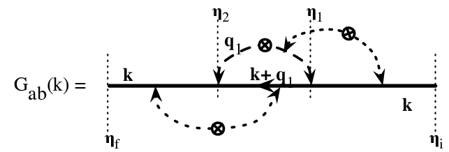
Figure 7: Large 𝐤{\bf k}, 𝐪1{\bf q}_{1} regularization of the one-loop diagram of the two-point propagator by higher order loops corrections in the high-kk limit. The main loop (in dashed line) is to be computed when 𝐪{\bf q} is in the UV domain.

The alternative prescription we propose is based on the following observation regarding the renormalization of the one-loop result: let us consider the diagram on Fig. 7 where the intermediate times η1′\eta^{\prime}_{1} and η2′\eta^{\prime}_{2} are fixed and the value of 𝐪1{\bf q}_{1} is also fixed such that its norm is large. The crucial observation we now make is that this object is then nothing but Γ(3)​(𝐪1,−𝐪1,𝐤,ηf,ηi)\Gamma^{(3)}({\bf q}_{1},-{\bf q}_{1},{\bf k},{\eta_{f}},{\eta_{i}}), where the three incoming modes from the initial conditions correspond to the two dashed lines (joined at the initial power spectrum, i.e. the ⊗\otimes symbol) and the rightmost kk-mode. But we now have a good understanding of its renormalization properties, given by Eq. (39). This equation tells us that we know how to resum all its loop corrections (some of which are represented by dotted loops in Fig. 7) in the large q1q_{1} and kk limit. Because it corresponds to the effects of long wavemodes, let us call this the infra-red (IR) correction. The expression we find is an application of the general result for multi-point propagator and it leads to a simple exp(−k2σdispl.2/2)\exp(-k^{2}{\sigma^{2}_{\rm displ.}}/2) factor. It is important to note that it is independent of q1q_{1} (and intermediate times η1\eta_{1} and η2\eta_{2}). We still have to perform the integral η1\eta_{1} and η2\eta_{2} and then over q1q_{1}. For the latter however we have to bear in mind that it cannot run over all possible values: it has to avoid its IR part. We can then split this integral into 2 parts, one IR, for which this result is not valid, and one UV for which it applies. Then the value of that set of diagrams would be

δGa+=e3​ηfa(I​R)(k)+e3​ηfa(U​V)(k)exp(−k2σdispl.2/2).\delta G_{a+}=e^{3\eta}f_{a}^{(IR)}(k)+e^{3\eta}f_{a}^{(UV)}(k)\exp\left(-k^{2}{\sigma^{2}_{\rm displ.}}/2\right). (45)

We then note that the first term is simply the first (non trivial) term of the usual IR resummation of diagrams, exp(−k2σdispl.2/2)\exp(-k^{2}{\sigma^{2}_{\rm displ.}}/2). We are then let to simply set

fa(I​R)​(k)\displaystyle f_{a}^{(IR)}(k) =\displaystyle= −12​k2​σdispl.2.\displaystyle-\frac{1}{2}k^{2}{\sigma^{2}_{\rm displ.}}. (46)
fa(U​V)​(k)\displaystyle f_{a}^{(UV)}(k) =\displaystyle= fa​(k)−fa(I​R)​(k).\displaystyle f_{a}(k)-f_{a}^{(IR)}(k). (47)

This identification leads to the following form,

Ga+reg=eη+δGa+=eη(1+e2​ηfa(k)+k2σdispl.2/2)exp(−k2σdispl.2/2)G_{a+}^{{\rm reg}}=e^{\eta}+\delta G_{a+}=e^{\eta}\left(1+e^{2\eta}f_{a}(k)+k^{2}{\sigma^{2}_{\rm displ.}}/2\right)\exp\left(-k^{2}{\sigma^{2}_{\rm displ.}}/2\right) (48)

for a “regularized” propagator which compared to the expression (44) amounts to replacing

exp⁡(e2​η​fa​(k)+k2​σdispl.2/2)→(1+e2​η​fa​(k)+k2​σdispl.2/2).\exp\left(e^{2\eta}f_{a}(k)+k^{2}{\sigma^{2}_{\rm displ.}}/2\right)\rightarrow(1+e^{2\eta}f_{a}(k)+k^{2}{\sigma^{2}_{\rm displ.}}/2). (49)

Note that these quantities are both finite at large kk. In Fig. 8, we compare these two prescriptions for the density and velocity fields at z=0z=0 for a Λ\Lambda-CDM cosmology. They are virtually indistinguishable when one considers the propagator shape. They significantly depart from one another only for k≃1​h−1​Mpck\simeq 1\,h^{-1}\,{\rm Mpc}, as shown on the right panel, that is at scales where the exponential damping is already extremely strong.

Refer to captionRefer to caption
Figure 8: Comparison of prescriptions for exponentiation schemes for the density (black upper lines) and velocity (brown lower lines) fields. The thin solid lines correspond to the RPT prescription, the thick dashed lines to this work. The left panel shows the propagators, the right corresponds to the propagator when they are divided by the global damping factor exp(−k2σdispl.2/2)\exp(-k^{2}{\sigma^{2}_{\rm displ.}}/2). The computations are made for z=0z=0 and for a Λ\Lambda-CDM cosmology (see Section V for details).

IV.2 The general prescription

Since the resummation properties of the Γ\Gamma functions preserve the topology and the intermediate time structure, the whole procedure applies to the full time dependence of the one-loop term. The integral splitting can then be done more generally and one gets,

Ga​breg​(k,ηf,ηi)\displaystyle G_{ab}^{{\rm reg}}(k,{\eta_{f}},{\eta_{i}}) =\displaystyle= [ga​b​(ηf,ηi)+δ​Ga​b1−loop​(k,ηf,ηi)+12​k2​σdispl.2​(ηf,ηi)​ga​b]​exp⁡(−k2​σdispl.2​(ηf,ηi)2).\displaystyle\left[g_{ab}({\eta_{f}},{\eta_{i}})+\delta G_{ab}^{{\rm 1-loop}}(k,{\eta_{f}},{\eta_{i}})+\frac{1}{2}k^{2}{\sigma^{2}_{\rm displ.}}({\eta_{f}},{\eta_{i}})g_{ab}\right]\exp\left(-\frac{k^{2}{\sigma^{2}_{\rm displ.}}({\eta_{f}},{\eta_{i}})}{2}\right). (50)

The relation with the RPT proposed forms given by Eqs. (38) is here more complicated. It is clear however that both propositions agree at the one-loop correction level and both propositions exhibit the same high-kk behavior.

One important aspect of this construction, which will be exploited in the following, is that it can obviously be extended to multipoint propagators,

Γa​b1​…​bpreg​(𝐤1,…,𝐤p,ηf,ηi)\displaystyle\Gamma^{{\rm reg}}_{ab_{1}\dots b_{p}}({\bf k}_{1},\dots,{\bf k}_{p},{\eta_{f}},{\eta_{i}}) =\displaystyle= [Γa​b1​…​bptree(𝐤1,…,𝐤p,ηf,ηi)+δΓa​b1​…​bp1−loop(𝐤1,…,𝐤p,ηf,ηi)+\displaystyle\left[\Gamma^{{\rm tree}}_{ab_{1}\dots b_{p}}({\bf k}_{1},\dots,{\bf k}_{p},{\eta_{f}},{\eta_{i}})+\delta\Gamma^{{\rm 1-loop}}_{ab_{1}\dots b_{p}}({\bf k}_{1},\dots,{\bf k}_{p},{\eta_{f}},{\eta_{i}})+\right. (51)
+12k2σdispl.2(ηf,ηi)Γa​b1​…​bptree(𝐤1,…,𝐤p,ηf,ηi)]exp(−k2​σdispl.2​(ηf,ηi)2)\displaystyle\hskip-56.9055pt\left.+\frac{1}{2}k^{2}{\sigma^{2}_{\rm displ.}}({\eta_{f}},{\eta_{i}})\Gamma^{{\rm tree}}_{ab_{1}\dots b_{p}}({\bf k}_{1},\dots,{\bf k}_{p},{\eta_{f}},{\eta_{i}})\right]\exp\left(-\frac{k^{2}{\sigma^{2}_{\rm displ.}}({\eta_{f}},{\eta_{i}})}{2}\right)

where k=|𝐤1+⋯+𝐤p|k=|{\bf k}_{1}+\dots+{\bf k}_{p}|. By construction this form is such that it has both the correct one-loop correction and the correct large-kk behavior. One can also remark that, unlike the RPT interpolation proposal where the matching is done in the “basis” given by density and velocity fields, the resulting form here is independent on the basis chosen to represent the cosmic fluids. This may not be an important difference for the CDM-only case but could be of importance when one wishes to extend the field content to other degrees of freedom (e.g. the case where one has in addition baryons, massive neutrinos, extra fields in the context of modified gravity theories, etc.)

Finally, another important advantage of this construction is that it can be pursued to any order in loop corrections in a rather straightforward way,

Γa​b1​…​bpreg=[Γa​b1​…​bptree+δΓa​b1​…​bp1−loop+12k2σdispl.2Γa​b1​…​bptree+δΓa​b1​…​bp2−loop+c.t.]exp(−k2​σdispl.22)\Gamma^{{\rm reg}}_{ab_{1}\dots b_{p}}=\left[\Gamma^{{\rm tree}}_{ab_{1}\dots b_{p}}+\delta\Gamma^{{\rm 1-loop}}_{ab_{1}\dots b_{p}}+\frac{1}{2}k^{2}{\sigma^{2}_{\rm displ.}}\Gamma^{{\rm tree}}_{ab_{1}\dots b_{p}}+\delta\Gamma^{{\rm 2-loop}}_{ab_{1}\dots b_{p}}+{\rm c.t.}\right]\exp\left(-\frac{k^{2}{\sigma^{2}_{\rm displ.}}}{2}\right) (52)

where c.t.{\rm c.t.} is a counter-term such that the 2-loop expression of the reg. expression is exact,

c.t.=−12​(k2​σdispl.22)2​Γa​b1​…​bptree+k2​σdispl.22​δ​Γa​b1​…​bp1−loop{\rm c.t.}=-\frac{1}{2}\left(\frac{k^{2}{\sigma^{2}_{\rm displ.}}}{2}\right)^{2}\Gamma^{{\rm tree}}_{ab_{1}\dots b_{p}}+\frac{k^{2}{\sigma^{2}_{\rm displ.}}}{2}\ \delta\Gamma^{{\rm 1-loop}}_{ab_{1}\dots b_{p}} (53)
Refer to captionRefer to captionRefer to captionRefer to caption
Figure 9: The shape of the Γ(2)\Gamma^{(2)} propagator for “equilateral” (k1=k2=k3=kk_{1}=k_{2}=k_{3}=k, top left), “colinear” (k1=k2=k/2k_{1}=k_{2}=k/2 ; k3=kk_{3}=k, top right), “anti-colinear” (k1=2​kk_{1}=2k ; k2=k3=kk_{2}=k_{3}=k, bottom left) and “squeezed” (k1=k2=4​kk_{1}=k_{2}=4k ; k3=kk_{3}=k, bottom right). The long dashed (blue) lines correspond to the simple exponential cut-off obtained in the high-k limit, Eq. (40), the short dashed (violet) lines are the tree plus one-loop order results and the solid (brown) line correspond to the interpolation scheme proposed this paper. These comparisons are made for a power spectrum corresponding to Λ−\Lambda-CDM model at z=0z=0.

Let us now illustrate this with some examples. The resulting interpolation scheme for Γ(2)\Gamma^{(2)} for specific geometries is shown in Fig. 9 for its late time behavior, showing that the interpolation is rather smooth. In particular it can handle the fact that tree-order and one-loop corrections have different signs. This is the case illustrated in the lower right panel in Fig. 9.

IV.3 The case of Non-Gaussian initial conditions

Refer to caption
Figure 10: Dominant complementary diagrams contributing to the one-point propagator in case of PNGs. They make intervene the primordial bispectrum Ba​b​c​(q1,q2,q3)B_{abc}(q_{1},q_{2},q_{3}). For models of cosmological interest they are of the order of the 2-loop contributions. When those diagrams are computed in the eikonal approximation, that is when the vertices are approximated by their high kk limit they all vanish for parity reasons. They do not so in general.

The case of PNGs can similarly be taken into account. In this case the damping factor is changed in order to take into account the higher order cumulants of the 1D displacement field as given in Eq. (30). Still it is possible to apply the same regularization scheme except that the counter terms have to be recomputed.

Novel two-loop order terms, depicted on Fig. 10, are due to the primordial bispectrum. In the eikonal approximation (e.g. when the vertex values are computed for qi≪kq_{i}\ll k), these diagrams vanish however. They therefore do not have counter terms in the regularization scheme we propose. Differences in the counter terms appear only at the three-loop order. It corresponds to the fact that the damping factor given by Eq. (30) is not sensitive to the primordial bispectrum, but it is to the primordial trispectrum.

V Comparison with numerical simulations

Refer to captionRefer to captionRefer to captionRefer to caption
Figure 11: Comparison of the proposed interpolation scheme against measurements of the two-point density propagator in numerical simulations at z=0z=0. Solid line is the prediction from Eq. (51) including the only most growing mode into Γ(2)​tree\Gamma^{(2){\rm tree}} and δ​Γ(2)​1−loop\delta\Gamma^{(2){\rm 1-loop}} after it is corrected for binning as discussed in the text; the dashed line is when the binning is not taken into account and the dotted line is the prediction when the one-loop correction is not taken into account. Symbols with error bars are the corresponding measurements in 50 runs of Lbox=1280​h−1L_{{\rm box}}=1280h^{-1} Mpc each. Different panels corresponds to different wave-vector configurations (or “triangle shapes”) as detailed in the y-axis labels (and main text). The results are plotted as a function of k=k3k=k_{3}.

As the prescription we are advocating here does not give significant differences for the two-point propagator (already studied in [12]) we focus our analysis in the three-point propagator.

As shown in the previous paragraph the prescriptions in Eqs. (51, 52) give non-trivial behaviors for the three-point propagator. These prescriptions can be compared against measurements in numerical simulations provided one can measure cross-bispectra between initial conditions δ0​(𝐤)\delta_{0}({\bf k}) and the final density fields δ⁡(𝐤,η)\delta({\bf k},\eta). The estimator for the three-point propagator was introduced in [10];

Γδ(2)​(k1,k2,k3)=12​P0​(k1)​P0​(k2)​1N​∑𝐤i​𝐤j∑𝐤lδ⁡(𝐤l,s)×δ0​(−𝐤i)​δ0​(−𝐤i),\Gamma^{(2)}_{\delta}(k_{1},k_{2},k_{3})=\frac{1}{2P_{0}(k_{1})P_{0}(k_{2})}\frac{1}{N}\sum_{{\bf k}_{i}{\bf k}_{j}}\sum_{{\bf k}_{l}}\delta({\bf k}_{l},s)\times\delta_{0}(-{\bf k}_{i})\delta_{0}(-{\bf k}_{i}), (54)

where the sum runs over Fourier modes 𝐤i{\bf k}_{i} in the |𝐤1||{\bf k}_{1}| bin, 𝐤j{\bf k}_{j} in the |𝐤2||{\bf k}_{2}| bin and 𝐤l{\bf k}_{l} in a bin |𝐤3||{\bf k}_{3}| such that |𝐤1−𝐤2|≤|𝐤3|≤𝐤1+𝐤2|{\bf k}_{1}-{\bf k}_{2}|\leq|{\bf k}_{3}|\leq{\bf k}_{1}+{\bf k}_{2}, and NN is the number of terms in the triple sum. Equation (54) is valid for initial conditions set in growing mode for which the only measurable quantity is the contraction Γa​b1​b2​ub1​ub2\Gamma_{ab_{1}b_{2}}u_{b_{1}}u_{b_{2}} with u=(1,1)u=(1,1) (and a=1=δa=1=\delta in our case). In addition it assumes Gaussian initial conditions, see [11] otherwise. We note that a similar expression holds for the velocity divergence propagator (i.e. a=2a=2), but its study is beyond the scope of this paper.

We used Eq. (54) to measure the three-point propagator in a set of 5050 N-body simulations, each containing Np​a​r=6403N_{par}=640^{3} particles within a comoving box-size of side Lb​o​x=1280​h−1​MpcL_{box}=1280h^{-1}{\rm Mpc}. The total comoving volume of our simulations is approximately 105​(h−1​Gpc)3105~(h^{-1}{\rm Gpc})^{3}. Cosmological parameters were chosen as Ωm=0.27\Omega_{m}=0.27, ΩΛ=0.73\Omega_{\Lambda}=0.73, Ωb=0.046\Omega_{b}=0.046 and h=0.72h=0.72, together with scalar spectral index ns=1n_{s}=1 and normalization σ8=0.9\sigma_{8}=0.9. The simulations were run using Gadget2 [20] with initial conditions set at zi=49z_{i}=49 using 2nd order Lagrangian Perturbation Theory (2LPT) [17, 21].

Before comparing theoretical predictions and numerical results it is important to account for binning effects since correlations of modes within bins implicitly change the shape of the predicted high-order propagators. Hence we will proceed by computing the predictions for binned modes. This is easily accomplished as follows. Let us denote by an overline the bin average, e.g.

Γ¯(2)​(k1,k2,k3)=1Nbin​P¯​(k1)​P¯​(k2)​∫ℬ1d3​𝐪1​∫ℬ2d3​𝐪2​∫ℬ3d3​𝐪3​P​(q1)​P​(q2)​Γ(2)​(q1,q2,q3)​δD​(𝐪3−𝐪1−𝐪2)\overline{\Gamma}^{(2)}(k_{1},k_{2},k_{3})=\frac{1}{N_{{\rm bin}}\overline{P}(k_{1})\overline{P}(k_{2})}\int_{{\cal B}_{1}}{\rm d}^{3}{\bf q}_{1}\int_{{\cal B}_{2}}{\rm d}^{3}{\bf q}_{2}\int_{{\cal B}_{3}}{\rm d}^{3}{\bf q}_{3}\,P(q_{1})\,P(q_{2})\,\Gamma^{(2)}(q_{1},q_{2},q_{3})\delta_{\rm D}({\bf q}_{3}-{\bf q}_{1}-{\bf q}_{2}) (55)

where 𝐪i{\bf q}_{i} is in bin ℬi={ki−δ​k/2,ki+δ​k/2}{\cal B}_{i}=\{k_{i}-\delta k/2,k_{i}+\delta k/2\} and NbinN_{{\rm bin}} is the normalization

Nbin=∫ℬ1d3​𝐪1​∫ℬ2d3​𝐪2​∫ℬ3d3​𝐪3​δD​(𝐪3−𝐪1−𝐪2),N_{{\rm bin}}=\int_{{\cal B}_{1}}{\rm d}^{3}{\bf q}_{1}\int_{{\cal B}_{2}}{\rm d}^{3}{\bf q}_{2}\int_{{\cal B}_{3}}{\rm d}^{3}{\bf q}_{3}\,\delta_{\rm D}({\bf q}_{3}-{\bf q}_{1}-{\bf q}_{2}), (56)

and

P¯​(ki)=∫ℬid3​𝐪i​P​(qi)/∫ℬid3​𝐪i.\overline{P}(k_{i})=\int_{{\cal B}_{i}}{\rm d}^{3}{\bf q}_{i}P(q_{i})/\int_{{\cal B}_{i}}{\rm d}^{3}{\bf q}_{i}. (57)

Then writing the Dirac δ\delta-function as δD(𝐤)=∫d3​𝐮(2​π)3exp(−i𝐤.𝐮)\delta_{\rm D}({\bf k})=\int\frac{{\rm d}^{3}{\bf u}}{(2\pi)^{3}}\exp(-{\rm i}{\bf k}.{\bf u}) we finally have,

Γ¯(2)​(k1,k2,k3)=32​πNbin​∫0∞u2​𝑑u​∫ℬ1q12​j0​(q1​u)​d​q1​∫ℬ2q22​j0​(q2​u)​d​q2​∫ℬ3q32​j0​(q3​u)​d​q3​Γ(2)​(q1,q2,q3)\overline{\Gamma}^{(2)}(k_{1},k_{2},k_{3})=\frac{32\pi}{N_{{\rm bin}}}\int_{0}^{\infty}u^{2}du\int_{{\cal B}_{1}}q_{1}^{2}\,j_{0}(q_{1}u)dq_{1}\int_{{\cal B}_{2}}q_{2}^{2}\,j_{0}(q_{2}u)dq_{2}\int_{{\cal B}_{3}}q_{3}^{2}\,j_{0}(q_{3}u)dq_{3}\ \Gamma^{(2)}(q_{1},q_{2},q_{3}) (58)

with Nbin≈8​π2​k1​k2​k3​(δ​k)3N_{{\rm bin}}\approx 8\pi^{2}k_{1}k_{2}k_{3}(\delta k)^{3}. This expression, where Γ(2)\Gamma^{(2)} is the model prediction from Eq. (51), is the one we use to compare with measurements obtained in numerical simulations. Notice that we are now using three wave-modes as arguments with 𝐤3=𝐤1+𝐤2{\bf k}_{3}={\bf k}_{1}+{\bf k}_{2} being the “outgoing” momenta. More precisely, in our computations we choose the central bin value to be ki=4​i×2​π/Lboxk_{i}=4\,i\times 2\pi/L_{{\rm box}} and the bin width to be fixed and given by δ​k=4×2​π/Lbox\delta k=4\times 2\pi/L_{{\rm box}}. Specific geometries, i.e. ratio of wave modes, are then defined from the central values of the bins.

Those comparisons are shown in Fig. 11 for four different shapes, “almost squeezed” (k1=k/4k_{1}=k/4 ; k2=k3=kk_{2}=k_{3}=k), “elongated” (k1=k/2k_{1}=k/2 ; k2=k3=kk_{2}=k_{3}=k), “equilateral” (where k1=k2=k3=kk_{1}=k_{2}=k_{3}=k) and “colinear” (k1=k2=k/2k_{1}=k_{2}=k/2 ; k3=kk_{3}=k). (Note that these configurations are not the same as in Fig. 9. This is due to the fact that the “anti-colinear” and “almost squeezed” configurations presented there exhibited too large signal-to-noise ratios). Remarkably all measured configurations show a very good agreement between the numerical results (points with error bars) and the proposed prescription (solid lines). The dashed lines show the prediction before the binning corrections. The latter can be quite large specifically at large scale (as expected) and furthermore in some configurations one-loop term corrections significantly improves the predictions when compared to the numerical results. One can also note that the size of the error bars change from configuration to configuration. This is due to the fact that, for a given k3k_{3} the number of available modes in all three bins vary strongly.

Overall, these results indicate that the proposed interpolation scheme works remarkably well when compared to measurements in simulations in an extended kk-range, which in turns is a very important step towards the accurate modeling of polyspectra.

VI Application: calculating the bispectrum

We are interested in the computation of Ba​b​c​(𝐤1,𝐤2,𝐤3)B_{abc}({\bf k}_{1},{\bf k}_{2},{\bf k}_{3}), the bispectrum of the components a,b,ca,b,c of the cosmic fluids,

⟨Ψa​(𝐤1,η)​Ψb​(𝐤2,η)​Ψc​(𝐤3,η)⟩=δD​(𝐤1+𝐤2+𝐤3)​Ba​b​c​(𝐤1,𝐤2,𝐤3,η)\big<\Psi_{a}({\bf k}_{1},\eta)\Psi_{b}({\bf k}_{2},\eta)\Psi_{c}({\bf k}_{3},\eta)\big>=\delta_{\rm D}({\bf k}_{1}+{\bf k}_{2}+{\bf k}_{3})\,B_{abc}({\bf k}_{1},{\bf k}_{2},{\bf k}_{3},\eta) (59)

Such bispectra can be computed from a resummation of product of Γ\Gamma functions. This is an extension of (25) and this is illustrated in Fig. 12. In particular if one wants to incorporate all one-loop effects one should include three types of diagrams: the first one involves the one-loop correction of the propagators, the second, third and fourth correspond to intrinsic one-loop contribution to the bispectra.

Refer to caption
Figure 12: The contributions to the bispectrum up to one loop order. In the first diagram the expressions of Γ(2)\Gamma^{(2)} and Γ(1)\Gamma^{(1)} should incorporate their own one loop correction ; they are computed using formulae (51) at one loop order. In the other 3 diagrams, the propagators correspond to their regularized tree order expressions; they are computed using formulae (40) . There is thus no need at this order to include their one-loop correction, in particular to Γ(3)\Gamma^{(3)}.

More precisely, for growing mode initial conditions, the bispectrum takes the form,

Ba​b​c​(𝐤1,𝐤2,𝐤3,η)\displaystyle B_{abc}({\bf k}_{1},{\bf k}_{2},{\bf k}_{3},\eta) =\displaystyle= 2​Γa++(2)​1−loop​(𝐤2,𝐤3,η)​Gb+1−loop​(𝐤2,η)​Gc+1−loop​(𝐤3,η)​P0​(k2)​P0​(k3)+sym.(2​terms)\displaystyle 2\,\Gamma^{(2){\rm 1-loop}}_{a++}({\bf k}_{2},{\bf k}_{3},\eta)G^{{\rm 1-loop}}_{b+}({\bf k}_{2},\eta)G^{{\rm 1-loop}}_{c+}({\bf k}_{3},\eta)P_{0}(k_{2})P_{0}(k_{3})+{\rm sym.}\ {\rm(2\ terms)} (60)
+\displaystyle+ 8​δD​(𝐤1+𝐪2−𝐪3)​δD​(𝐤2+𝐪3−𝐪1)​δD​(𝐤3+𝐪1+𝐪2)​P0​(q1)​P0​(q2)​P0​(q3)\displaystyle 8\,\delta_{\rm D}({\bf k}_{1}+{\bf q}_{2}-{\bf q}_{3})\,\delta_{\rm D}({\bf k}_{2}+{\bf q}_{3}-{\bf q}_{1})\,\delta_{\rm D}({\bf k}_{3}+{\bf q}_{1}+{\bf q}_{2})\,P_{0}(q_{1})\,P_{0}(q_{2})\,P_{0}(q_{3})
×Γa++(2)​tree​(𝐪3,−𝐪2,η)​Γb++(2)​tree​(𝐪1,−𝐪3,η)​Γc++(2)​tree​(𝐪2,−𝐪1,η)+sym.(2​terms)\displaystyle\hskip 14.22636pt\times\,\Gamma^{(2)\,{\rm tree}}_{a++}({\bf q}_{3},-{\bf q}_{2},\eta)\,\Gamma^{(2)\,{\rm tree}}_{b++}({\bf q}_{1},-{\bf q}_{3},\eta)\,\Gamma^{(2)\,{\rm tree}}_{c++}({\bf q}_{2},-{\bf q}_{1},\eta)+{\rm sym.}\ {\rm(2\ terms)}
+\displaystyle+ 12​Γa+++(3)​tree​(−𝐤2+𝐪,−𝐪,−𝐤3,η)​Γb++(2)​tree​(𝐤2−𝐪,𝐪,η)​Gc+tree​(𝐤3,η)\displaystyle 12\,\Gamma^{(3)\,{\rm tree}}_{a+++}(-{\bf k}_{2}+{\bf q},-{\bf q},-{\bf k}_{3},\eta)\,\Gamma^{(2)\,{\rm tree}}_{b++}({\bf k}_{2}-{\bf q},{\bf q},\eta)\,G^{{\rm tree}}_{c+}({\bf k}_{3},\eta)
×P0​(|𝐤2−𝐪|)​P0​(q)​P0​(k3)+sym.(2​terms)\displaystyle\hskip 14.22636pt\times\,P_{0}(|{\bf k}_{2}-{\bf q}|)\,P_{0}(q)\,P_{0}(k_{3})+{\rm sym.}\ {\rm(2\ terms)}

where all the propagators are computed using their regularized form, whether it is at tree order as in (40) or including one-loop correction as in (51). Integrals over the wavevectors 𝐪1{\bf q}_{1}, 𝐪2{\bf q}_{2} and 𝐪3{\bf q}_{3} when present are implicit, and the symmetric terms are obtained by a simultaneous permutation of the indices a​b​cabc and the wave modes 𝐤1{\bf k}_{1}, 𝐤2{\bf k}_{2} and 𝐤3{\bf k}_{3}. Note that in this formulation the Γ(p)\Gamma^{(p)} functions are assumed to be symmetric functions of their arguments. Because of that the last 2 diagrams that appear in Fig. 12 are automatically included.

For its practical evaluation the non trivial part is the one-loop expression of the Γa++(2)\Gamma_{a++}^{(2)} propagators. Its properties were discussed in [10]. We give in the appendix their actual values for both the density and the velocity fields. They are the crucial ingredient to use to compute the bispectrum at one-loop order.

Refer to captionRefer to captionRefer to caption
Figure 13: The shape of the density bispectrum, B111​(k1,k2,k3)B_{111}(k_{1},k_{2},k_{3}), as a function of scale for different configurations of the wavevectors. The (gray) dotted line is the standard tree order prediction for the bispectrum and the (gray) dot-dashed the standard one-loop result; the (green) short dashed line corresponds to the first contribution in the diagrammatic expansion of Fig. 12, the (red) long dashed line to the 2 others and the solid line the resulting reconstructed bispectrum. The first panel shows k3​B​(k,k,k)k^{3}B(k,k,k), e.g. equilateral configuration. The second corresponds to a lightly squeezed configuration, k3​B​(k/2,k,k)k^{3}B(k/2,k,k), and the last to a flatten configuration, k3​B​(2​k,k,k)k^{3}B(2k,k,k). The predictions are made for z=0.5z=0.5.
Refer to caption
Figure 14: The reduced bispectrum as a function of the relative angle between the wave-vectors θ\theta for k1=0.1​hk_{1}=0.1h/Mpc and k2=0.2​hk_{2}=0.2h/Mpc. Lines follow the same convention as in Fig. 13.

We present in Figs. 13 and 14 the resulting shape of the density bispectrum for a standard Λ\LambdaCDM model at z=0.5z=0.5. Figure 13 shows the scale dependence of the bispectrum (multiplied by k3k^{3} to make it less scale dependent). It makes clear that the contribution of the first diagram and that of the 3 others correspond to different scales, each producing one bump at different scales. This is reminiscent to what the RPT calculations give for the power spectrum [2].

In turn, Fig 14 explores the resulting angular dependence of the reduced bispectrum. Here we plot

Q⁡(k1,k2,k3)=1P0​(k1)​P0​(k2)+P0​(k2)​P0​(k3)+P0​(k3)​P0​(k1)​B111​(𝐤1,𝐤2,𝐤3)Q(k_{1},k_{2},k_{3})=\frac{1}{P_{0}(k_{1})P_{0}(k_{2})+P_{0}(k_{2})P_{0}(k_{3})+P_{0}(k_{3})P_{0}(k_{1})}B_{111}({\bf k}_{1},{\bf k}_{2},{\bf k}_{3}) (61)

where the expression of the power spectrum is kept at linear order. The result is expressed for fixed values of k1=0.1​hk_{1}=0.1\,h/Mpc and k2=0.2​hk_{2}=0.2\,h/Mpc and as a function of their relative angle, θ\theta, so that k32=k12+k22+2​k1​k2​cos⁡θk_{3}^{2}=k_{1}^{2}+k_{2}^{2}+2k_{1}k_{2}\cos\theta. The plot compares the naked “tree” order result (dotted line) with our prediction or the perturbative calculations (same convention as in Fig. 13). Detailed comparisons of such predictions with NN-body results is left for future studies.

VII Conclusions

In this paper we propose a systematic interpolation scheme that aims at describing the (multi-point) propagators in such a way that their expressions interpolate between their perturbation theory forms - to any loop order - and their large-kk behavior obtained from non-perturbative re-summations. This scheme is based on a separation of scales between the long wave-modes, whose effects are fully resumed and lead to the large-kk behavior, and the short wave-modes that are fully taken into account in the perturbation theory treatment. Our prescription is different from the exponentiation scheme proposed in [12] but departs from it only very weakly. Our new prescription however is very general and can be used for any loop order calculations and for any propagator. Furthermore, this construction is totally unambiguous. We note that it can even be used in the context of primordial non-Gaussianities although new terms arise only at two loop order.

As the construction proposed here has a very general range of application, it should in principle be tested for a large variety of quantities, from two-point and multi-point propagators of the density field to the ones for the velocity field. We proposed here some comparisons with N-body results for the quantities that are of most interest for the use of the multi-point propagators in the context of the Γ\Gamma-expansion applied to the calculation of the density power spectrum. Because of the property we mentioned in the previous paragraph, this prescription for the two-point propagator is found to give very accurate results for the two-point propagator. We leave for further studies the impact of two-loop effects. In this work we further check the validity of our prescription against numerical results for the one-loop level of the density three-point propagator. These comparisons are presented in Fig. 11. We found that it gives a satisfactory form for a large range of configurations, i.e. interpolating the low-kk one-loop result with the high-kk exponential decay, even when the signs of tree order and one-loop forms differ.

In the context of the Γ\Gamma-expansion approach this construction therefore provides us with the necessary recipes for constructing poly-spectra incorporating any order of perturbation theory results. In coming papers we will explicitly compare predictions of the Γ\Gamma-expansion for the power spectra with numerical simulations when higher order PT loop corrections are included. These prescriptions provide a good opportunity for giving the explicit form of the bispectra in the context of the Γ\Gamma-expansion. The explicit mathematical forms are given in Section VI when bispectra are computed up to one-loop order. Such expressions make use in particular of the three-point propagators at one-loop order whose explicit forms are given in the appendix. We found in particular that the bispectra terms can be separated in a tree order contribution and coupling terms contributions that contribute at different scales, i.e. in subsequent bumps, in a similar way to the power spectrum. Comparison of the proposed forms for the bispectrum with NN-body results is however left for further studies.

We finally note that such a construction is restricted here to the case of a single pressure-less fluid. Whether it could be used in cases the fluid content of the universe is richer (with extra degrees of freedom carried by baryons, see [22, 13], massive neutrinos, dark energy components, see [23, 24], etc.) is still largely an open issue. Results obtained in [13] however suggest that the effects of adiabatic long wavelength modes can be resummed and therefore could be incorporated in a large variety of cases.

Acknowledgements.
We thank the Programme National de Cosmologie et Galaxies for their support. M.C. acknowledges support by the Spanish Ministerio de Ciencia e Innovacion (MICINN), project AYA2009-13936, Consolider-Ingenio CSD2007- 00060, European Commission Marie Curie Initial Training Network CosmoComp (PITN-GA-2009-238356), research project 2009-SGR-1398 from Generalitat de Catalunya and the Juan de la Cierva MICINN program. R.S. was partially supported by grants NSF AST-1109432 and NASA NNA10A171G.

References

  • [1] F. Bernardeau, S. Colombi, E. Gaztañaga, and R. Scoccimarro, Phys. Rep. 367, 1 (2002).
  • [2] M. Crocce and R. Scoccimarro, Phys. Rev. D 73, 063519 (2006a), eprint astro-ph/0509418.
  • [3] M. Pietroni, Journal of Cosmology and Astro-Particle Physics 10, 36 (2008), eprint 0806.0971.
  • [4] T. Hiramatsu and A. Taruya, Phys. Rev. D 79, 103526 (2009), eprint 0902.3772.
  • [5] A. Taruya and T. Hiramatsu, Astrophys. J.  674, 617 (2008), eprint 0708.1367.
  • [6] T. Matsubara, Phys. Rev. D 77, 063530 (2008), eprint 0711.2521.
  • [7] F. Bernardeau and P. Valageas, Phys. Rev. D 78, 083503 (2008), eprint 0805.0805.
  • [8] T. Okamura, A. Taruya, and T. Matsubara, Journal of Cosmology and Astro-Particle Physics 8, 12 (2011), eprint 1105.1491.
  • [9] T. Matsubara, Phys. Rev. D 83, 083518 (2011), eprint 1102.4619.
  • [10] F. Bernardeau, M. Crocce, and R. Scoccimarro, Phys. Rev. D 78, 103521 (2008), eprint 0806.2334.
  • [11] F. Bernardeau, M. Crocce, and E. Sefusatti, Phys. Rev. D 82, 083507 (2010), eprint 1006.4656.
  • [12] M. Crocce and R. Scoccimarro, Phys. Rev. D 73, 063520 (2006b), eprint astro-ph/0509419.
  • [13] F. Bernardeau, N. Van de Rijt, and F. Vernizzi, ArXiv e-prints (2011), eprint 1109.3400.
  • [14] P. McDonald, ArXiv e-prints (2009), eprint 0910.1002.
  • [15] D. Baumann, A. Nicolis, L. Senatore, and M. Zaldarriaga, ArXiv e-prints (2010), eprint 1004.2488.
  • [16] M. Pietroni, G. Mangano, N. Saviano, and M. Viel, ArXiv e-prints (2011), eprint 1108.5203.
  • [17] R. Scoccimarro, Mon. Not. R. Astr. Soc. 299, 1097 (1998), eprint arXiv:astro-ph/9711187.
  • [18] R. Scoccimarro, in The Onset of Nonlinearity in Cosmology, edited by J. N. Fry, J. R. Buchler, and H. Kandrup (2001), vol. 927 of New York Academy Sciences Annals, pp. 13–+.
  • [19] S. Anselmi, S. Matarrese, and M. Pietroni, JCAP 6, 15 (2011), eprint 1011.4477.
  • [20] V. Springel, Mon. Not. R. Astr. Soc. 364, 1105 (2005), eprint arXiv:astro-ph/0505010.
  • [21] M. Crocce, S. Pueblas, and R. Scoccimarro, Mon. Not. R. Astr. Soc. 373, 369 (2006), eprint arXiv:astro-ph/0606505.
  • [22] G. Somogyi and R. E. Smith, Phys. Rev. D 81, 023524 (2010), eprint 0910.5220.
  • [23] F. Bernardeau and P. Brax, Journal of Cosmology and Astro-Particle Physics 6, 19 (2011), eprint 1102.1907.
  • [24] E. Sefusatti and F. Vernizzi, Journal of Cosmology and Astro-Particle Physics 3, 47 (2011), eprint 1101.1026.

Appendix A Explicit expression of the one-loop Γ(2)\Gamma^{(2)} propagators

We give here the explicit expressions of the late time component (most growing term) of the 1-loop expression of the three-point propagator (for growing mode initial conditions). The final result is obtained by the explicit integration over the wave mode qq depending on the linear power spectrum P0​(q)P_{0}(q),

Γ1++(2)​1−loop​(k1,k2,k3)=4​π​e4​η​∫q2​𝑑q​Γ1++(2)​1−loop​(k1,k2,k3,q)​P0​(q)\Gamma^{(2){\rm 1-loop}}_{1++}(k_{1},k_{2},k_{3})=4\pi e^{4\eta}\int q^{2}{\rm d}q\Gamma^{(2){\rm 1-loop}}_{1++}(k_{1},k_{2},k_{3},q)\,P_{0}(q) (62)

where the result is expressed in terms of the 3 norms, k1k_{1}, k2k_{2}, k3k_{3} so that k32=k12+k22+2​𝐤1.𝐤2k_{3}^{2}=k_{1}^{2}+k_{2}^{2}+2{\bf k}_{1}.{\bf k}_{2}. Note that these three norms obey the triangular inequality.

Note that Γi++(2)​1−loop​(k1,k2,k3,q)\Gamma^{(2){\rm 1-loop}}_{i++}(k_{1},k_{2},k_{3},q) obeys the following asymptotic behaviors,

Γi++(2)​1−loop​(k1,k2,k3,q)\displaystyle\Gamma^{(2){\rm 1-loop}}_{i++}(k_{1},k_{2},k_{3},q) →\displaystyle\to −k326​q2​Γi++(2)​tree​(k1,k2,k3),\displaystyle-\frac{k_{3}^{2}}{6q^{2}}\Gamma^{(2){\rm tree}}_{i++}(k_{1},k_{2},k_{3}), (63)

and q→0q\to 0. We also have

Γ1++(2)​1−loop​(𝐤1,𝐤2)\displaystyle\Gamma^{(2){\rm 1-loop}}_{1++}({\bf k}_{1},{\bf k}_{2}) →\displaystyle\to 𝐤1.𝐤22​k12​f​(k2),\displaystyle\frac{{\bf k}_{1}.{\bf k}_{2}}{2k_{1}^{2}}f(k_{2}), (64)
Γ2++(2)​1−loop​(𝐤1,𝐤2)\displaystyle\Gamma^{(2){\rm 1-loop}}_{2++}({\bf k}_{1},{\bf k}_{2}) →\displaystyle\to 𝐤1.𝐤22​k12​g​(k2),\displaystyle\frac{{\bf k}_{1}.{\bf k}_{2}}{2k_{1}^{2}}g(k_{2}), (65)

when 𝐤1→0{\bf k}_{1}\to 0 and where the functions f⁡(k)f(k) and g⁡(k)g(k) are defined in Eqs. (). These 2 asymptotic regimes can be used as internal checks.

The function Γ1++(2)​1−loop​(k1,k2,k3,q)\Gamma^{(2){\rm 1-loop}}_{1++}(k_{1},k_{2},k_{3},q) has been obtained after integration of the angular variable in the loop expressions. The result can be expressed in terms of the functions

ℒ⁡(k1)\displaystyle{\cal L}\left(k_{1}\right) =\displaystyle= log⁡(k1+q)2(k1−q)2\displaystyle\log\frac{(k_{1}+q)^{2}}{(k_{1}-q)^{2}} (66)
𝒲⁡(k1,k2,k3)\displaystyle{\cal W}\left(k_{1},k_{2},k_{3}\right) =\displaystyle= log⁡(−4​k32​q2−2​(k12−q2)​(k22−q2)−4​k3​q​(−k12−k22+k32)​q2+k12​k22+q4−4​k32​q2−2​(k12−q2)​(k22−q2)+4​k3​q​(−k12−k22+k32)​q2+k12​k22+q4)\displaystyle\log\left(\frac{-4k_{3}^{2}q^{2}-2\left(k_{1}^{2}-q^{2}\right)\left(k_{2}^{2}-q^{2}\right)-4k_{3}q\sqrt{\left(-k_{1}^{2}-k_{2}^{2}+k_{3}^{2}\right)q^{2}+k_{1}^{2}k_{2}^{2}+q^{4}}}{-4k_{3}^{2}q^{2}-2\left(k_{1}^{2}-q^{2}\right)\left(k_{2}^{2}-q^{2}\right)+4k_{3}q\sqrt{\left(-k_{1}^{2}-k_{2}^{2}+k_{3}^{2}\right)q^{2}+k_{1}^{2}k_{2}^{2}+q^{4}}}\right) (67)

and it reads,

Γ1++(2)​1−loop​(k1,k2,k3,q)=\displaystyle\Gamma^{(2){\rm 1-loop}}_{1++}(k_{1},k_{2},k_{3},q)=
k2​(k12−q2)2​(7​k32​q2+2​k34−9​q4)29568​k12​q5​q2​(k22−k32+q2)+k12​(k32−q2)​𝒲​(k1,k3,k2)+sym.(k1↔k2)\displaystyle\frac{k_{2}\left(k_{1}^{2}-q^{2}\right)^{2}\left(7k_{3}^{2}q^{2}+2k_{3}^{4}-9q^{4}\right)}{29568\ k_{1}^{2}q^{5}\sqrt{q^{2}\left(k_{2}^{2}-k_{3}^{2}+q^{2}\right)+k_{1}^{2}\left(k_{3}^{2}-q^{2}\right)}}\ {\cal W}\left(k_{1},k_{3},k_{2}\right)+{\rm sym.}{\rm\ (k_{1}\leftrightarrow k_{2})}
+3​k33​(k12−q2)2​(k22−q2)217248​k12​k22​q5​q2​(−k22+k32+q2)+k12​(k22−q2)​𝒲​(k1,k2,k3)\displaystyle+\frac{3k_{3}^{3}\left(k_{1}^{2}-q^{2}\right)^{2}\left(k_{2}^{2}-q^{2}\right)^{2}}{17248\ k_{1}^{2}k_{2}^{2}q^{5}\sqrt{q^{2}\left(-k_{2}^{2}+k_{3}^{2}+q^{2}\right)+k_{1}^{2}\left(k_{2}^{2}-q^{2}\right)}}\ {\cal W}\left(k_{1},k_{2},k_{3}\right)
−(k12−q2)21655808​k19​k22​q5[165(k22−k32)3q6−k110(582k22+791k32+1947q2)+\displaystyle-\frac{\left(k_{1}^{2}-q^{2}\right)^{2}}{1655808\ k_{1}^{9}k_{2}^{2}q^{5}}\ \left[165\left(k_{2}^{2}-k_{3}^{2}\right)^{3}q^{6}-k_{1}^{10}\left(582k_{2}^{2}+791k_{3}^{2}+1947q^{2}\right)+\right.
+k16​(−1113​k32​q4+179​k34​q2−3​k24​(211​k32+2155​q2)+k22​(758​k32​q2+390​k34−7284​q4)+492​k26+151​k36+219​q6)\displaystyle\hskip 14.22636pt\left.+k_{1}^{6}\left(-1113k_{3}^{2}q^{4}+179k_{3}^{4}q^{2}-3k_{2}^{4}\left(211k_{3}^{2}+2155q^{2}\right)+k_{2}^{2}\left(758k_{3}^{2}q^{2}+390k_{3}^{4}-7284q^{4}\right)+492k_{2}^{6}+151k_{3}^{6}+219q^{6}\right)\right.
+k18​(1787​k32​q2+k22​(2120​k32+6891​q2)+51​k24+601​k34+1689​q4)\displaystyle\hskip 14.22636pt\left.+k_{1}^{8}\left(1787k_{3}^{2}q^{2}+k_{2}^{2}\left(2120k_{3}^{2}+6891q^{2}\right)+51k_{2}^{4}+601k_{3}^{4}+1689q^{4}\right)\right.
+k14​q2​(405​k32​q4+k24​(7269​q2−1677​k32)−321​k34​q2+k22​(−4376​k32​q2+391​k34+471​q4)+1017​k26+269​k36)\displaystyle\hskip 14.22636pt\left.+k_{1}^{4}q^{2}\left(405k_{3}^{2}q^{4}+k_{2}^{4}\left(7269q^{2}-1677k_{3}^{2}\right)-321k_{3}^{4}q^{2}+k_{2}^{2}\left(-4376k_{3}^{2}q^{2}+391k_{3}^{4}+471q^{4}\right)+1017k_{2}^{6}+269k_{3}^{6}\right)\right.
−3(k22−k32)k12q4(k22(285q2−473k32)−17(9k32q2+5k34)+558k24)+39k112]ℒ(k1)+sym.(k1↔k2)\displaystyle\hskip 14.22636pt\left.-3\left(k_{2}^{2}-k_{3}^{2}\right)k_{1}^{2}q^{4}\left(k_{2}^{2}\left(285q^{2}-473k_{3}^{2}\right)-17\left(9k_{3}^{2}q^{2}+5k_{3}^{4}\right)+558k_{2}^{4}\right)+39k_{1}^{12}\right]\ {\cal L}\left(k_{1}\right)+{\rm sym.}{\rm\ (k_{1}\leftrightarrow k_{2})}
+(7​k32​q2+2​k34−9​q4)236544​k12​k22​k35​q5[−12(k12−k22)2q6−3(k12−k22)2(k12+k22)q4\displaystyle+\frac{\left(7k_{3}^{2}q^{2}+2k_{3}^{4}-9q^{4}\right)}{236544\ k_{1}^{2}k_{2}^{2}k_{3}^{5}q^{5}}\left[-12\left(k_{1}^{2}-k_{2}^{2}\right)^{2}q^{6}-3\left(k_{1}^{2}-k_{2}^{2}\right)^{2}\left(k_{1}^{2}+k_{2}^{2}\right)q^{4}\right.
−2​k310−15​(k12+k22)​k38+k36​(46​(k12+k22)​q2+16​(k12−k22)2−2​q4)\displaystyle\hskip 14.22636pt\left.-2k_{3}^{10}-15\left(k_{1}^{2}+k_{2}^{2}\right)k_{3}^{8}+k_{3}^{6}\left(46\left(k_{1}^{2}+k_{2}^{2}\right)q^{2}+16\left(k_{1}^{2}-k_{2}^{2}\right)^{2}-2q^{4}\right)\right.
+k34​(−47​(k12+k22)​q4−8​(7​k14−17​k22​k12+7​k24)​q2+(k12+k22)​(k14−10​k22​k12+k24)+4​q6)\displaystyle\hskip 14.22636pt\left.+k_{3}^{4}\left(-47\left(k_{1}^{2}+k_{2}^{2}\right)q^{4}-8\left(7k_{1}^{4}-17k_{2}^{2}k_{1}^{2}+7k_{2}^{4}\right)q^{2}+\left(k_{1}^{2}+k_{2}^{2}\right)\left(k_{1}^{4}-10k_{2}^{2}k_{1}^{2}+k_{2}^{4}\right)+4q^{6}\right)\right.
+k32(8(k12+k22)q6+(52k14−96k22k12+52k24)q4+2(k12−k22)2(k12+k22)q2)]ℒ(k3)\displaystyle\hskip 14.22636pt\left.+k_{3}^{2}\left(8\left(k_{1}^{2}+k_{2}^{2}\right)q^{6}+\left(52k_{1}^{4}-96k_{2}^{2}k_{1}^{2}+52k_{2}^{4}\right)q^{4}+2\left(k_{1}^{2}-k_{2}^{2}\right)^{2}\left(k_{1}^{2}+k_{2}^{2}\right)q^{2}\right)\right]{\cal L}\left(k_{3}\right)
+16209280​q4​k18​k28​k34{420k16k26k312\displaystyle+\frac{1}{{6209280\ q^{4}k_{1}^{8}k_{2}^{8}k_{3}^{4}}}\left\{420k_{1}^{6}k_{2}^{6}k_{3}^{12}\right.
+[−2475(k16+k26)q8+300k12k22(k14+k24)q6+9090k14k24(k12+k22)q4\displaystyle\hskip 14.22636pt\left.+\left[-2475\left(k_{1}^{6}+k_{2}^{6}\right)q^{8}+300k_{1}^{2}k_{2}^{2}\left(k_{1}^{4}+k_{2}^{4}\right)q^{6}+9090k_{1}^{4}k_{2}^{4}\left(k_{1}^{2}+k_{2}^{2}\right)q^{4}\right.\right.
−68910k16k26q2+5415k16k26(k12+k22)]k310\displaystyle\hskip 28.45274pt\left.\left.-68910k_{1}^{6}k_{2}^{6}q^{2}+5415k_{1}^{6}k_{2}^{6}\left(k_{1}^{2}+k_{2}^{2}\right)\right]k_{3}^{10}\right.
+[135(55k18−51k22k16−51k26k12+55k28)q8−45k12k22(k12+k22)(663k14−811k22k12+663k24)q6\displaystyle\hskip 14.22636pt\left.+\left[135\left(55k_{1}^{8}-51k_{2}^{2}k_{1}^{6}-51k_{2}^{6}k_{1}^{2}+55k_{2}^{8}\right)q^{8}-45k_{1}^{2}k_{2}^{2}\left(k_{1}^{2}+k_{2}^{2}\right)\left(663k_{1}^{4}-811k_{2}^{2}k_{1}^{2}+663k_{2}^{4}\right)q^{6}\right.\right.
+(38925​k24​k18+9532​k26​k16+38925​k28​k14)​q4−120370​k16​k26​(k12+k22)​q2\displaystyle\hskip 28.45274pt\left.\left.+\left(38925k_{2}^{4}k_{1}^{8}+9532k_{2}^{6}k_{1}^{6}+38925k_{2}^{8}k_{1}^{4}\right)q^{4}-120370k_{1}^{6}k_{2}^{6}\left(k_{1}^{2}+k_{2}^{2}\right)q^{2}\right.\right.
+15k16k26(377k14+940k22k12+377k24)]k38\displaystyle\hskip 28.45274pt\left.\left.+15k_{1}^{6}k_{2}^{6}\left(377k_{1}^{4}+940k_{2}^{2}k_{1}^{2}+377k_{2}^{4}\right)\right]k_{3}^{8}\right.
+[−135(k12+k22)(55k18−201k22k16+156k24k14−201k26k12+55k28)q8\displaystyle\hskip 14.22636pt\left.+\left[-135\left(k_{1}^{2}+k_{2}^{2}\right)\left(55k_{1}^{8}-201k_{2}^{2}k_{1}^{6}+156k_{2}^{4}k_{1}^{4}-201k_{2}^{6}k_{1}^{2}+55k_{2}^{8}\right)q^{8}\right.\right.
+30​k12​k22​(1959​k18−3283​k22​k16−1907​k24​k14−3283​k26​k12+1959​k28)​q6\displaystyle\hskip 28.45274pt\left.\left.+30k_{1}^{2}k_{2}^{2}\left(1959k_{1}^{8}-3283k_{2}^{2}k_{1}^{6}-1907k_{2}^{4}k_{1}^{4}-3283k_{2}^{6}k_{1}^{2}+1959k_{2}^{8}\right)q^{6}\right.\right.
−2​k14​k24​(k12+k22)​(53220​k14−178337​k22​k12+53220​k24)​q4\displaystyle\hskip 28.45274pt\left.\left.-2k_{1}^{4}k_{2}^{4}\left(k_{1}^{2}+k_{2}^{2}\right)\left(53220k_{1}^{4}-178337k_{2}^{2}k_{1}^{2}+53220k_{2}^{4}\right)q^{4}\right.\right.
+10k16k26(22261k14−45566k22k12+22261k24)q2−15k16k26(k12+k22)(805k14−2306k22k12+805k24)]k36\displaystyle\hskip 28.45274pt\left.\left.+10k_{1}^{6}k_{2}^{6}\left(22261k_{1}^{4}-45566k_{2}^{2}k_{1}^{2}+22261k_{2}^{4}\right)q^{2}-15k_{1}^{6}k_{2}^{6}\left(k_{1}^{2}+k_{2}^{2}\right)\left(805k_{1}^{4}-2306k_{2}^{2}k_{1}^{2}+805k_{2}^{4}\right)\right]k_{3}^{6}\right.
+[45(55k112−285k22k110+157k24k18+230k26k16+157k28k14−285k210k12+55k212)q8\displaystyle\hskip 14.22636pt\left.+\left[45\left(55k_{1}^{12}-285k_{2}^{2}k_{1}^{10}+157k_{2}^{4}k_{1}^{8}+230k_{2}^{6}k_{1}^{6}+157k_{2}^{8}k_{1}^{4}-285k_{2}^{10}k_{1}^{2}+55k_{2}^{12}\right)q^{8}\right.\right.
−15​k12​k22​(k12+k22)​(1949​k18−10643​k22​k16+20573​k24​k14−10643​k26​k12+1949​k28)​q6\displaystyle\hskip 28.45274pt\left.\left.-15k_{1}^{2}k_{2}^{2}\left(k_{1}^{2}+k_{2}^{2}\right)\left(1949k_{1}^{8}-10643k_{2}^{2}k_{1}^{6}+20573k_{2}^{4}k_{1}^{4}-10643k_{2}^{6}k_{1}^{2}+1949k_{2}^{8}\right)q^{6}\right.\right.
+3​k14​k24​(19475​k18−139742​k22​k16+246974​k24​k14−139742​k26​k12+19475​k28)​q4\displaystyle\hskip 28.45274pt\left.\left.+3k_{1}^{4}k_{2}^{4}\left(19475k_{1}^{8}-139742k_{2}^{2}k_{1}^{6}+246974k_{2}^{4}k_{1}^{4}-139742k_{2}^{6}k_{1}^{2}+19475k_{2}^{8}\right)q^{4}\right.\right.
−30k16k26(k12+k22)(911k14−1570k22k12+911k24)q2+45k16k26(k12−k22)(13k14−4k22k12+13k24)2]k34\displaystyle\hskip 28.45274pt\left.\left.-30k_{1}^{6}k_{2}^{6}\left(k_{1}^{2}+k_{2}^{2}\right)\left(911k_{1}^{4}-1570k_{2}^{2}k_{1}^{2}+911k_{2}^{4}\right)q^{2}+45k_{1}^{6}k_{2}^{6}\left(k_{1}^{2}-k_{2}^{2}\right){}^{2}\left(13k_{1}^{4}-4k_{2}^{2}k_{1}^{2}+13k_{2}^{4}\right)\right]k_{3}^{4}\right.
+[7560​k16​k26​(k12+k22)​q8+1260​k16​k26​(43​k14−80​k22​k12+43​k24)​q6+3150​k16​k26​(k12−k22)2​(k12+k22)​q4]​k32\displaystyle\hskip 14.22636pt\left.+\left[7560k_{1}^{6}k_{2}^{6}\left(k_{1}^{2}+k_{2}^{2}\right)q^{8}+1260k_{1}^{6}k_{2}^{6}\left(43k_{1}^{4}-80k_{2}^{2}k_{1}^{2}+43k_{2}^{4}\right)q^{6}+3150k_{1}^{6}k_{2}^{6}\left(k_{1}^{2}-k_{2}^{2}\right)^{2}\left(k_{1}^{2}+k_{2}^{2}\right)q^{4}\right]k_{3}^{2}\right.
−11340q8k16k26(k12−k22)2−2835q6k16k26(k12−k22)2(k12+k22)}.\displaystyle\hskip 14.22636pt\left.-11340q^{8}k_{1}^{6}k_{2}^{6}\left(k_{1}^{2}-k_{2}^{2}\right)^{2}-2835q^{6}k_{1}^{6}k_{2}^{6}\left(k_{1}^{2}-k_{2}^{2}\right)^{2}\left(k_{1}^{2}+k_{2}^{2}\right)\right\}. (68)

It can be noted that the final expression is symmetric in k1k_{1} and k2k_{2}. The velocity component can be similarly constructed,

Γ2++(2)​1−loop​(k1,k2,k3,q)=\displaystyle\Gamma^{(2){\rm 1-loop}}_{2++}(k_{1},k_{2},k_{3},q)=
k2​(k12−q2)2​(−5​k32​q2+8​k34−3​q4)29568​k12​q5​q2​(k22−k32+q2)+k12​(k32−q2)​𝒲​(k1,k3,k2)+sym.(k1↔k2)\displaystyle\frac{k_{2}\left(k_{1}^{2}-q^{2}\right)^{2}\left(-5k_{3}^{2}q^{2}+8k_{3}^{4}-3q^{4}\right)}{29568\ k_{1}^{2}q^{5}\sqrt{q^{2}\left(k_{2}^{2}-k_{3}^{2}+q^{2}\right)+k_{1}^{2}\left(k_{3}^{2}-q^{2}\right)}}\ {\cal W}\left(k_{1},k_{3},k_{2}\right)+{\rm sym.}{\rm\ (k_{1}\leftrightarrow k_{2})}
+3​k33​(k12−q2)2​(k22−q2)24312​k12​k22​q5​q2​(−k22+k32+q2)+k12​(k22−q2)​𝒲​(k1,k2,k3)\displaystyle+\frac{3k_{3}^{3}\left(k_{1}^{2}-q^{2}\right)^{2}\left(k_{2}^{2}-q^{2}\right)^{2}}{4312\ k_{1}^{2}k_{2}^{2}q^{5}\sqrt{q^{2}\left(-k_{2}^{2}+k_{3}^{2}+q^{2}\right)+k_{1}^{2}\left(k_{2}^{2}-q^{2}\right)}}\ {\cal W}\left(k_{1},k_{2},k_{3}\right)
−(k12−q2)21655808​k19​k22​q5[55(k22−k32)q63−k110(194k22+1921k32+649q2)+13k112\displaystyle-\frac{\left(k_{1}^{2}-q^{2}\right)^{2}}{1655808\ k_{1}^{9}k_{2}^{2}q^{5}}\ \left[55\left(k_{2}^{2}-k_{3}^{2}\right){}^{3}q^{6}-k_{1}^{10}\left(194k_{2}^{2}+1921k_{3}^{2}+649q^{2}\right)+13k_{1}^{12}\right.
+k16​(25​k32​q4−1759​k34​q2+k24​(801​k32−2155​q2)+k22​(−3414​k32​q2+306​k34−2428​q4)+164​k26+329​k36+73​q6)\displaystyle\hskip 14.22636pt\left.+k_{1}^{6}\left(25k_{3}^{2}q^{4}-1759k_{3}^{4}q^{2}+k_{2}^{4}\left(801k_{3}^{2}-2155q^{2}\right)+k_{2}^{2}\left(-3414k_{3}^{2}q^{2}+306k_{3}^{4}-2428q^{4}\right)+164k_{2}^{6}+329k_{3}^{6}+73q^{6}\right)\right.
+k18​(2913​k32​q2+k22​(1176​k32+2297​q2)+17​k24+1579​k34+563​q4)\displaystyle\hskip 14.22636pt\left.+k_{1}^{8}\left(2913k_{3}^{2}q^{2}+k_{2}^{2}\left(1176k_{3}^{2}+2297q^{2}\right)+17k_{2}^{4}+1579k_{3}^{4}+563q^{4}\right)\right.
+k14​q2​(135​k32​q4+k24​(321​k32+2423​q2)+333​k34​q2+k22​(−784​k32​q2−1307​k34+157​q4)+339​k26+647​k36)\displaystyle\hskip 14.22636pt\left.+k_{1}^{4}q^{2}\left(135k_{3}^{2}q^{4}+k_{2}^{4}\left(321k_{3}^{2}+2423q^{2}\right)+333k_{3}^{4}q^{2}+k_{2}^{2}\left(-784k_{3}^{2}q^{2}-1307k_{3}^{4}+157q^{4}\right)+339k_{2}^{6}+647k_{3}^{6}\right)\right.
−3(k22−k32)k12q4(k22(121k32+95q2)−51k32q2+186k24−307k34)]ℒ(k1)+sym.(k1↔k2)\displaystyle\hskip 14.22636pt\left.-3\left(k_{2}^{2}-k_{3}^{2}\right)k_{1}^{2}q^{4}\left(k_{2}^{2}\left(121k_{3}^{2}+95q^{2}\right)-51k_{3}^{2}q^{2}+186k_{2}^{4}-307k_{3}^{4}\right)\right]\ {\cal L}\left(k_{1}\right)+{\rm sym.}{\rm\ (k_{1}\leftrightarrow k_{2})}
+(−5​k32​q2+8​k34−3​q4)236544​k12​k22​k35​q5[−12(k12−k22)2q6−3(k12−k22)2(k12+k22)q4\displaystyle+\frac{\left(-5k_{3}^{2}q^{2}+8k_{3}^{4}-3q^{4}\right)}{236544\ k_{1}^{2}k_{2}^{2}k_{3}^{5}q^{5}}\left[-12\left(k_{1}^{2}-k_{2}^{2}\right)^{2}q^{6}-3\left(k_{1}^{2}-k_{2}^{2}\right)^{2}\left(k_{1}^{2}+k_{2}^{2}\right)q^{4}\right.
−2​k310−15​(k12+k22)​k38+k36​(46​(k12+k22)​q2+16​(k12−k22)2−2​q4)\displaystyle\hskip 14.22636pt\left.-2k_{3}^{10}-15\left(k_{1}^{2}+k_{2}^{2}\right)k_{3}^{8}+k_{3}^{6}\left(46\left(k_{1}^{2}+k_{2}^{2}\right)q^{2}+16\left(k_{1}^{2}-k_{2}^{2}\right)^{2}-2q^{4}\right)\right.
+k34​(−47​(k12+k22)​q4−8​(7​k14−17​k22​k12+7​k24)​q2+(k12+k22)​(k14−10​k22​k12+k24)+4​q6)\displaystyle\hskip 14.22636pt\left.+k_{3}^{4}\left(-47\left(k_{1}^{2}+k_{2}^{2}\right)q^{4}-8\left(7k_{1}^{4}-17k_{2}^{2}k_{1}^{2}+7k_{2}^{4}\right)q^{2}+\left(k_{1}^{2}+k_{2}^{2}\right)\left(k_{1}^{4}-10k_{2}^{2}k_{1}^{2}+k_{2}^{4}\right)+4q^{6}\right)\right.
+k32(8(k12+k22)q6+(52k14−96k22k12+52k24)q4+2(k12−k22)2(k12+k22)q2)]ℒ(k3)\displaystyle\hskip 14.22636pt\left.+k_{3}^{2}\left(8\left(k_{1}^{2}+k_{2}^{2}\right)q^{6}+\left(52k_{1}^{4}-96k_{2}^{2}k_{1}^{2}+52k_{2}^{4}\right)q^{4}+2\left(k_{1}^{2}-k_{2}^{2}\right)^{2}\left(k_{1}^{2}+k_{2}^{2}\right)q^{2}\right)\right]{\cal L}\left(k_{3}\right)
+16209280​q4​k18​k28​k34{1680k16k26k312\displaystyle+\frac{1}{{6209280\ q^{4}k_{1}^{8}k_{2}^{8}k_{3}^{4}}}\left\{1680k_{1}^{6}k_{2}^{6}k_{3}^{12}\right.
+(−825​(k16+k26)​q8−12440​k12​k22​(k14+k24)​q6+32290​k14​k24​(k12+k22)​q4CLOSE\displaystyle\hskip 14.22636pt\left.+\left(-825\left(k_{1}^{6}+k_{2}^{6}\right)q^{8}-12440k_{1}^{2}k_{2}^{2}\left(k_{1}^{4}+k_{2}^{4}\right)q^{6}+32290k_{1}^{4}k_{2}^{4}\left(k_{1}^{2}+k_{2}^{2}\right)q^{4}\right.\right.
OPEN−133850​k16​k26​q2+17535​k16​k26​(k12+k22))​k310\displaystyle\hskip 28.45274pt\left.\left.-133850k_{1}^{6}k_{2}^{6}q^{2}+17535k_{1}^{6}k_{2}^{6}\left(k_{1}^{2}+k_{2}^{2}\right)\right)k_{3}^{10}\right.
+(45​(55​k18−51​k22​k16−51​k26​k12+55​k28)​q8+15​k12​k22​(k12+k22)​(1009​k14−421​k22​k12+1009​k24)​q6CLOSE\displaystyle\hskip 14.22636pt\left.+\left(45\left(55k_{1}^{8}-51k_{2}^{2}k_{1}^{6}-51k_{2}^{6}k_{1}^{2}+55k_{2}^{8}\right)q^{8}+15k_{1}^{2}k_{2}^{2}\left(k_{1}^{2}+k_{2}^{2}\right)\left(1009k_{1}^{4}-421k_{2}^{2}k_{1}^{2}+1009k_{2}^{4}\right)q^{6}\right.\right.
−k14​k24​(50385​k14+92816​k22​k12+50385​k24)​q4−81190​k16​k26​(k12+k22)​q2\displaystyle\hskip 28.45274pt\left.\left.-k_{1}^{4}k_{2}^{4}\left(50385k_{1}^{4}+92816k_{2}^{2}k_{1}^{2}+50385k_{2}^{4}\right)q^{4}-81190k_{1}^{6}k_{2}^{6}\left(k_{1}^{2}+k_{2}^{2}\right)q^{2}\right.\right.
OPEN+15​k16​k26​(683​k14+1252​k22​k12+683​k24))​k38\displaystyle\hskip 28.45274pt\left.\left.+15k_{1}^{6}k_{2}^{6}\left(683k_{1}^{4}+1252k_{2}^{2}k_{1}^{2}+683k_{2}^{4}\right)\right)k_{3}^{8}\right.
+(−45​(k12+k22)​(55​k18−201​k22​k16+156​k24​k14−201​k26​k12+55​k28)​q8CLOSE\displaystyle\hskip 14.22636pt\left.+\left(-45\left(k_{1}^{2}+k_{2}^{2}\right)\left(55k_{1}^{8}-201k_{2}^{2}k_{1}^{6}+156k_{2}^{4}k_{1}^{4}-201k_{2}^{6}k_{1}^{2}+55k_{2}^{8}\right)q^{8}\right.\right.
+30​k12​k22​(235​k18−757​k22​k16−137​k24​k14−757​k26​k12+235​k28)​q6\displaystyle\hskip 28.45274pt\left.\left.+30k_{1}^{2}k_{2}^{2}\left(235k_{1}^{8}-757k_{2}^{2}k_{1}^{6}-137k_{2}^{4}k_{1}^{4}-757k_{2}^{6}k_{1}^{2}+235k_{2}^{8}\right)q^{6}\right.\right.
−4​k14​k24​(k12+k22)​(345​k14+628​k22​k12+345​k24)​q4\displaystyle\hskip 28.45274pt\left.\left.-4k_{1}^{4}k_{2}^{4}\left(k_{1}^{2}+k_{2}^{2}\right)\left(345k_{1}^{4}+628k_{2}^{2}k_{1}^{2}+345k_{2}^{4}\right)q^{4}\right.\right.
OPEN+10​k16​k26​(24507​k14−50506​k22​k12+24507​k24)​q2−15​k16​k26​(k12+k22)​(1977​k14−4010​k22​k12+1977​k24))​k36\displaystyle\hskip 28.45274pt\left.\left.+10k_{1}^{6}k_{2}^{6}\left(24507k_{1}^{4}-50506k_{2}^{2}k_{1}^{2}+24507k_{2}^{4}\right)q^{2}-15k_{1}^{6}k_{2}^{6}\left(k_{1}^{2}+k_{2}^{2}\right)\left(1977k_{1}^{4}-4010k_{2}^{2}k_{1}^{2}+1977k_{2}^{4}\right)\right)k_{3}^{6}\right.
+(15​(55​k112−285​k22​k110+157​k24​k18+230​k26​k16+157​k28​k14−285​k210​k12+55​k212)​q8CLOSE\displaystyle\hskip 14.22636pt\left.+\left(15\left(55k_{1}^{12}-285k_{2}^{2}k_{1}^{10}+157k_{2}^{4}k_{1}^{8}+230k_{2}^{6}k_{1}^{6}+157k_{2}^{8}k_{1}^{4}-285k_{2}^{10}k_{1}^{2}+55k_{2}^{12}\right)q^{8}\right.\right.
−5​k12​k22​(k12+k22)​(1949​k18−10643​k22​k16+19341​k24​k14−10643​k26​k12+1949​k28)​q6\displaystyle\hskip 28.45274pt\left.\left.-5k_{1}^{2}k_{2}^{2}\left(k_{1}^{2}+k_{2}^{2}\right)\left(1949k_{1}^{8}-10643k_{2}^{2}k_{1}^{6}+19341k_{2}^{4}k_{1}^{4}-10643k_{2}^{6}k_{1}^{2}+1949k_{2}^{8}\right)q^{6}\right.\right.
+k14​k24​(19475​k18−93542​k22​k16+160734​k24​k14−93542​k26​k12+19475​k28)​q4\displaystyle\hskip 28.45274pt\left.\left.+k_{1}^{4}k_{2}^{4}\left(19475k_{1}^{8}-93542k_{2}^{2}k_{1}^{6}+160734k_{2}^{4}k_{1}^{4}-93542k_{2}^{6}k_{1}^{2}+19475k_{2}^{8}\right)q^{4}\right.\right.
−90k16k26(k12+k22)(67k14−106k22k12+67k24)q2+15k16k26(k12−k22)(13k14−4k22k12+13k24)2)k34\displaystyle\hskip 28.45274pt\left.\left.-90k_{1}^{6}k_{2}^{6}\left(k_{1}^{2}+k_{2}^{2}\right)\left(67k_{1}^{4}-106k_{2}^{2}k_{1}^{2}+67k_{2}^{4}\right)q^{2}+15k_{1}^{6}k_{2}^{6}\left(k_{1}^{2}-k_{2}^{2}\right){}^{2}\left(13k_{1}^{4}-4k_{2}^{2}k_{1}^{2}+13k_{2}^{4}\right)\right)k_{3}^{4}\right.
+(2520k16k26(k12+k22)q8+1260k16k26(7k14−12k22k12+7k24)q6−1260k16k26(k12−k22)(k12+k22)2q4)k32\displaystyle\hskip 14.22636pt\left.+\left(2520k_{1}^{6}k_{2}^{6}\left(k_{1}^{2}+k_{2}^{2}\right)q^{8}+1260k_{1}^{6}k_{2}^{6}\left(7k_{1}^{4}-12k_{2}^{2}k_{1}^{2}+7k_{2}^{4}\right)q^{6}-1260k_{1}^{6}k_{2}^{6}\left(k_{1}^{2}-k_{2}^{2}\right){}^{2}\left(k_{1}^{2}+k_{2}^{2}\right)q^{4}\right)k_{3}^{2}\right.
−3780q8k16k26(k12−k22)−2945q6k16k26(k12−k22)(k12+k22)2}.\displaystyle\hskip 14.22636pt\left.-3780q^{8}k_{1}^{6}k_{2}^{6}\left(k_{1}^{2}-k_{2}^{2}\right){}^{2}-945q^{6}k_{1}^{6}k_{2}^{6}\left(k_{1}^{2}-k_{2}^{2}\right){}^{2}\left(k_{1}^{2}+k_{2}^{2}\right)\right\}. (69)