跳到论文正文
W Papers独立论文阅读器 arXiv:1112.3455 论文正文 计算阅读时间 · 0%
引用这篇论文根据当前论文元数据生成,正式投稿前建议核对。


License: arXiv.org perpetual non-exclusive license
arXiv:1112.3455v3 [math.LO] 17 May 2013

Resource control and strong normalisation

S. Ghilezan ††thanks: Email:˜gsilvia@uns.ac.rs Affiliation: University of Novi Sad, Faculty of Technical Sciences, Serbia    J. Ivetić ††thanks: Email:˜jelenaivetic@uns.ac.rs Affiliation: University of Novi Sad, Faculty of Technical Sciences, Serbia    P. Lescanne ††thanks: Email:˜pierre.lescanne@ens-lyon.fr Affiliation: University of Lyon, École Normal Supérieure de Lyon, France    S. Likavec ††thanks: Email:˜likavec@di.unito.it Affiliation: Dipartimento di Informatica, Università di Torino, Italy
August 24, 2026
Abstract

We introduce the resource control cube, a system consisting of eight intuitionistic lambda calculi with either implicit or explicit control of resources and with either natural deduction or sequent calculus. The four calculi of the cube that correspond to natural deduction have been proposed by Kesner and Renaud and the four calculi that correspond to sequent lambda calculi are introduced in this paper. The presentation is parameterized with the set of resources (weakening or contraction), which enables a uniform treatment of the eight calculi of the cube. The simply typed resource control cube, on the one hand, expands the Curry-Howard correspondence to intuitionistic natural deduction and intuitionistic sequent logic with implicit or explicit structural rules and, on the other hand, is related to substructural logics.

We propose a general intersection type system for the resource control cube calculi. Our main contribution is a characterisation of strong normalisation of reductions in this cube. First, we prove that typeability implies strong normalisation in the “natural deduction base” of the cube by adapting the reducibility method. We then prove that typeability implies strong normalisation in the “sequent base” of the cube by using a combination of well-orders and a suitable embedding in the “natural deduction base”. Finally, we prove that strong normalisation implies typeability in the cube using head subject expansion. All proofs are general and can be made specific to each calculus of the cube by instantiating the set of resources.

Keywords: lambda calculus, sequent calculus, resource control, intersection types, strong normalisation

1998 ACM Subject Classification: F.4.1 [Mathematical Logic]: Lambda calculus and related systems, F.3.1 [Specifying and Verifying and Reasoning about Programs]: Logics of programs, F.3.2 [Semantics of Programming Languages]: Operational semantics, F.3.3 [Studies of Program Constructs]: Type structure

Introduction

Curry–Howard correspondence or formulae-as-types and proofs-as-programs paradigm [How80], establishes a fundamental connection between various logical and computational systems. Simply typed λ\lambda-calculus provides the computational interpretation of intuitionistic natural deduction where simplifying a proof corresponds to a program execution. The correspondence between sequent calculus derivations and natural deduction derivations is not a one-to-one map: several cut-free derivations correspond to one normal derivation [BG00]. Starting from Griffin’s extension of the Curry–Howard correspondence to classical logic [Gri90], this connection has been extended to other calculi and logical systems. For instance, Parigot’s λ​μ\lambda\mu-calculus [Par92] corresponds to classical natural deduction and as such inspired investigation into the relationship between classical logic and theories of control in programming languages [Par97, dG94, OS97, Bie98, AH03, HG08]. In the realm of sequent calculus, Herbelin’s λ¯\overline{\lambda}-calculus [Her95] and Espírito Santo’s λ𝖦𝗍𝗓\lambda^{\mathsf{Gtz}}-calculus [Esp07a] correspond to intuitionistic sequent calculus, whereas Barbanera and Berardi’s symmetric calculus [BB96] and Curien and Herbelin’s λ¯​μ​μ~\overline{\lambda}\mu\widetilde{\mu}-calculus [CH00] correspond to its classical variants. An extensive overview of this subject can be found in [SU06, GL09].

Our intention is to bring this correspondence to the calculi with control operators, namely erasure and duplication, which correspond to weakening and contraction on the logical side. The wish to control the use of variables in a λ\lambda-term can be traced back to Church [Chu41] who introduced the λ​I\lambda I-calculus. According to Church, the variables bound by λ\lambda abstraction should occur in the term at least once. More recently, following the ideas of linear logic [Gir87], van Oostrom [vO01] proposed to extend the λ\lambda-calculus, and Kesner and Lengrand [KL07] proposed to extend the λ\lambdax-calculus with explicit substitution, with operators to tightly control the use of variables (resources). Resource control in sequent calculus corresponding to classical logic was proposed in [Ž07]. Resource control both in λ\lambda-calculus and λ\lambdax-calculus is proposed in [KR09, KR11], whereas resource control for sequent λ\lambda-calculus is proposed in [GILŽ11, GILL11]. Like in the λ​I\lambda I-calculus, bound variables must still occur in the term, but if a variable xx is not used in a term MM this can be expressed by using the expression x⊙Mx\odot M where the operator ⊙\odot is called erasure (aka weakening). In this way, the term MM does not contain the variable xx, but the term x⊙Mx\odot M does. Similarly, a variable should not occur twice. If nevertheless, we want to have two positions for the same variable, we have to duplicate it explicitly, using fresh names. This is done by using the operator x<x1x2x<^{x_{1}}_{x_{2}}\ , called duplication (aka contraction) which creates two fresh variables x1x_{1} and x2x_{2}. Extending the classical λ\lambda-calculus and the sequent λ\lambda-calculus λ𝖦𝗍𝗓\lambda^{\mathsf{Gtz}} with explicit erasure and duplication provides the Curry–Howard correspondence for intuitionistic natural deduction and intuitionistic sequent calculus with explicit structural rules, as investigated in [KL07, KR09, KR11, GILŽ11]. The notation used in this paper is along the lines of [Ž07] and close to [vO01].

A different approach to the resource aware lambda calculus, motivated mostly by the development of the process calculi, was investigated by Boudol in [Bou93]. Instead of extending the syntax of λ\lambda-calculus with explicit resource operators, Boudol proposed a non-deterministic calculus with a generalised notion of application. In his work, a function is applied to a structure called a bag, having the form (N1m1​|…|​Nkmk)(N^{m_{1}}_{1}|...|N^{m_{k}}_{k}) in which Ni,i=1,…,kN_{i},\;i=1,...,k are resources and mi∈ℕ∪{∞},i=1,…,km_{i}\in\mathbb{N}\cup\{\infty\},\;i=1,...,k are multiplicities, representing the maximum possible number of the resource usage. In this framework, the usual application is written as M​N∞MN^{\infty}. The theory was further developed in [BCL99], connected to linear logic via differential λ\lambda-calculus in [ER03] and even typed with non-idempotent intersection types in [PR10].

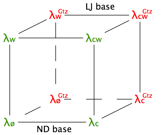
Our contribution is inspired by Kesner and Lengrand’s [KL07] and Kesner and Renaud’s [KR09, KR11] work on resource operators for λ\lambda-calculus. The linear λ​𝗅𝗑𝗋\lambda\mathsf{lxr} calculus of Kesner and Lengrand introduces operators for substitution, erasure and duplication, preserving at the same time strong normalisation, confluence and subject reduction property of its predecessor λ​𝗑{\lambda\mathsf{x}} [BR95]. This approach is then generalised in Kesner and Renaud’s Prismoid of Resources [KR09, KR11] by considering various combinations in which these three operators are made explicit or implicit. In this paper we introduce the notion of resource control cube, consisting of two systems λℛ\lambda_{\mathcal{R}} and λℛ𝖦𝗍𝗓\lambda^{\mathsf{Gtz}}_{\mathcal{R}}, which can be seen as two opposite sides of the cube (see Figure 1). In λℛ\lambda_{\mathcal{R}} we consider four calculi, each of which is obtained by making erasure (aka weakening) or duplication (aka contraction) explicit or implicit. In λℛ𝖦𝗍𝗓\lambda^{\mathsf{Gtz}}_{\mathcal{R}} we consider the four sequent style counterparts of the λℛ\lambda_{\mathcal{R}}-calculi. We will call the λℛ\lambda_{\mathcal{R}} system the natural deduction ND-base of the cube, and the λℛ𝖦𝗍𝗓\lambda^{\mathsf{Gtz}}_{\mathcal{R}} system the sequent LJ-base of the cube11 1 We are aware that our notation is not symmetric, since 𝖦𝗍𝗓\mathsf{Gtz} is specified explicitly for the LJ-base but 𝖭𝖣\mathsf{ND} is not for the ND-base. This was a conscious decision because ND-base contains ordinary λ\lambda-calculus where correspondence with natural deduction is not explicitly written.. Explicit control of erasure and duplication leads to decomposing of reduction steps into more atomic ones, thus revealing details of computation which are usually left implicit. Since erasing and duplicating of (sub)terms essentially changes the structure of a program, it is important to see how this mechanism really works and to be able to control this part of computation.
Refer to caption
Figure 1: Resource control cube

Let us turn our attention to type assignment systems for various term calculi. The basic type assignment system is the one with simple types in which the only forming operator is an arrow →\rightarrow. Among many extensions of this type assignment system, the one that characterises the largest class of terms, is the extension with intersection types, where a new type forming operator ∩\cap is introduced. The principal feature of this operator is the possibility to assign two different types to a certain term at the same time. The intersection types have been originally introduced in [CDC78, Sal78, CDC80, Pot80, CDCV80] in order to characterise termination properties of various term calculi [vB92, Gal98, Ghi96]. The extension of Curry–Howard correspondence to other formalisms brought the need for intersection types into many different settings [DGL08, Kik07, Mat00, Nee05].

We introduce the intersection types into all eight calculi of the resource control cube. Our intersection type assignment systems λℛ∩\lambda_{\mathcal{R}}\cap and λℛ𝖦𝗍𝗓∩\lambda^{\mathsf{Gtz}}_{\mathcal{R}}\cap integrate intersections into logical rules, thus preserving syntax-directedness of the systems. We assign a restricted form of intersection types to terms, namely strict types, therefore eliminating the need for pre-order on types. Using these intersection type assignment systems we manage to completely characterise strong normalisation in the cube by proving that terms in all calculi in both bases enjoy the strong normalisation property if and only if they are typeable. While this characterization is well-known for the pure λ\lambda-calculus and λ𝖦𝗍𝗓\lambda^{\mathsf{Gtz}}-calculus, it is a new result for the other six calculi of the cube. The paper proves the characterization in a modular way, presenting one uniform proof for the first four calculi in natural deduction style, and one uniform proof for the four sequent style calculi. Concerning the sequent calculus, to the best of our knowledge, there is no literature on explicit resource control operators for λ𝖦𝗍𝗓\lambda^{\mathsf{Gtz}}-calculus, nor on the connection to intersection types (except for the initial version of this work presented in [GILL11]).

The rest of the paper is organised as follows. In Section 1 we introduce the untyped resource control cube which consists of eight calculi λℛ\lambda_{\mathcal{R}} and λℛ𝖦𝗍𝗓\lambda^{\mathsf{Gtz}}_{\mathcal{R}} with different combinations of explicit/implicit control operators of weakening and contraction. Basic type assignment systems with simple types for these calculi are given in Section 2. Intersection type assignment systems with strict types are introduced in Section 3. By adapting the reducibility method to explicit resource control operators, we first prove that typeable terms are strongly normalising in λℛ\lambda_{\mathcal{R}}-calculi of the ND-base in Section 4. Next, we prove that typeability implies strong normalization in λℛ𝖦𝗍𝗓\lambda^{\mathsf{Gtz}}_{\mathcal{R}}-calculi of the LJ-base by using a combination of well-orders and a suitable embedding of λℛ𝖦𝗍𝗓\lambda^{\mathsf{Gtz}}_{\mathcal{R}}-terms into λℛ\lambda_{\mathcal{R}}-terms which preserves types and enables the simulation of all the reductions in λℛ𝖦𝗍𝗓\lambda^{\mathsf{Gtz}}_{\mathcal{R}}-calculi by the operational semantics of the λℛ\lambda_{\mathcal{R}}-calculi. Finally, in Section 5, we prove that strong normalisation implies typeability in both systems using head subject expansion. We conclude in Section 6.

1 Untyped resource control cube

1.1 Resource control lambda calculi λℛ\lambda_{\mathcal{R}}

In this section we present four calculi obtained by adding contraction and weakening to the λ\lambda-calculus either as explicit or implicit operators. We denote these four calculi by λℛ\lambda_{\mathcal{R}}, where ℛ⊆{𝖼,𝗐}\mathcal{R}\subseteq\{\mathsf{c},\mathsf{w}\} and 𝖼\mathsf{c}, 𝗐\mathsf{w} denote explicit contraction and weakening, respectively. The presented system operationally corresponds to the four calculi of the so-called implicit base of Kesner and Renaud’s prismoid [KR09], as will be showed in Section 1.2. We use a notation along the lines of [Ž07] and close to [vO01]. It is slightly modified w.r.t. [KR09] in order to emphasize the correspondence between these calculi and their sequent counterparts.22 2 Note that in [KR09], instead of considering the sequent counterparts, the authors consider the so called explicit base, i.e. the four corresponding calculi with explicit substitutions. For the convenience of the reader and to avoid repetition, we present all the calculi in a uniform way. This implies that some constructions or features are part of one calculus and not of the others. When a feature occurs in a calculus associated with the operator r∈ℛ\textsf{r}\in\mathcal{R} and is ignored elsewhere, we put this feature between brackets indexed by the symbol r. For instance, if we write [x∈Fv(f)]𝗐[x\in Fv(f)]_{\mathsf{w}}, this means that the condition x∈F​v​(f)x\in Fv(f) appears only in the calculus which contains explicit weakening, as seen from the index w.

In order to define the terms of the calculus, we introduce a syntactic category called pre-terms. A pre-term can be a variable, an abstraction, an application, a contraction or a weakening. The abstract syntax of the λℛ\lambda_{\mathcal{R}} pre-terms is given by the following:

Pre-termsf:⁣:=x|λx.f|ff|x<x1x2f|x⊙f\begin{array}[]{lcrcl}\textsf{Pre-terms}&&f&::=&x\,|\,\lambda x.f\,|\,ff\,|\,x<^{x_{1}}_{x_{2}}f\,|\,x\odot f\\ \end{array}

where xx ranges over a denumerable set of term variables

The list of free variables of a pre-term ff, denoted by F​v​[f]Fv[f], is defined as follows (where l,ml,m denotes appending two lists and l∖xl\setminus x denotes removing all occurrences of an element from a list):

Fv[x]=x;Fv[λx.f]=Fv[f]∖x;Fv[fg]=Fv[f],Fv[g];[F​v​[x⊙f]=x,F​v​[f]]𝗐;[Fv[x<x1x2f]={F​v​[f],x1∉F​v​[f]​and;x2∉F​v​[f]x,(F​v​[f]∖{x1,x2}),x1∈F​v​[f]​or​x2∈F​v​[f]]𝖼\begin{array}[]{c}Fv[x]=x;\quad Fv[\lambda x.f]=Fv[f]\setminus x;\quad Fv[fg]=Fv[f],Fv[g];\\ \left[Fv[x\odot f]=x,Fv[f]\right]_{\mathsf{w}};\\ \left[Fv[x<^{x_{1}}_{x_{2}}f]=\left\{\begin{array}[]{rl}Fv[f],&x_{1}\notin Fv[f]\;\;\mbox{and};\;x_{2}\notin Fv[f]\\ x,(Fv[f]\setminus\{x_{1},x_{2}\}),&x_{1}\in Fv[f]\;\;\mbox{or}\;\;x_{2}\in Fv[f]\end{array}\right.\right]_{\mathsf{c}}\end{array}

The set of free variables, denoted by F​v​(f)Fv(f), is extracted out of the list F​v​[f]Fv[f], by un-ordering the list and removing multiple occurrences of each variable, if any. The set of bound variables of a pre-term ff, denoted by B​v​(f)Bv(f), contains all variables of ff that are not free in it, i.e. B​v​(f)=V​a​r​(f)∖F​v​(f)Bv(f)=Var(f)\setminus Fv(f). In x<x1x2fx<^{x_{1}}_{x_{2}}f, the duplication binds the variables x1x_{1} and x2x_{2} in ff and introduces a fresh variable xx if at least one of x1,x2x_{1},x_{2} is free in ff. In x⊙fx\odot f, the variable xx is free. In order to avoid parentheses, we let the scope of all binders extend to the right as much as possible.

The sets of λℛ\lambda_{\mathcal{R}}-terms, denoted by Λℛ\Lambda_{\mathcal{R}}, are subsets of the set of pre-terms and are defined by the inference rules given in Figure 2. In the reminder of the paper, we will use M,N,P​…M,N,P... to denote terms. We also use the notation X⊙MX\odot M for x1⊙…​xn⊙Mx_{1}\odot...\;x_{n}\odot M and X<YZMX<^{Y}_{Z}M for x1<y1z1…xn<ynznMx_{1}<^{y_{1}}_{z_{1}}...\;x_{n}<^{y_{n}}_{z_{n}}M, where XX, YY and ZZ are lists of size nn, consisting of all distinct variables x1,…,xn,y1,…,yn,z1,…,znx_{1},...,x_{n},y_{1},...,y_{n},z_{1},...,z_{n}. If n=0n=0, i.e., if XX is the empty list, then X⊙M=X<YZM=MX\odot M=X<^{Y}_{Z}M=M. In particular, given a term NN, we use a specific notation: Fv[N]<F​V​N2F​v​(N1)M[N/x1,N/x2]Fv[N]<^{Fv(N_{1})}_{FV{N_{2}}}M[N/x_{1},N/x_{2}]. Assume that NN has the list F​v​(N)=(z1,…,zp)Fv(N)=(z_{1},...,z_{p}) as free variables. We write NN as N⁡(z1,…,zp)N(z_{1},...,z_{p}) and N1N_{1} and N2N_{2}, as the term in which the variables have been renamed with fresh variables. I.e., N1=N⁡(z1,1,…​z1,p)N_{1}=N(z_{1,1},...z_{1,p}) and N2=N⁡(z2,1,…​z2,p)N_{2}=N(z_{2,1},...z_{2,p}).

Fv[N]<F​V​N2F​v​(N1)M[N/x1,N/x2]Fv[N]<^{Fv(N_{1})}_{FV{N_{2}}}M[N/x_{1},N/x_{2}]

is by definition:

z1<z2,1z1,1…zp<z2,pz1,pM[N(z1,1,…z1,p)/x1][N(z2,1,…z2,p)/x2].z_{1}<^{z_{1,1}}_{z_{2,1}}...z_{p}<^{z_{1,p}}_{z_{2,p}}\,M[N(z_{1,1},...z_{1,p})/x_{1}][N(z_{2,1},...z_{2,p})/x_{2}].

Note that due to the equivalence relation defined in Figure 5, we can use these notations also for a set of triple of variables, all distinct.

(v​a​r)x∈Λℛ‾f∈Λℛ[x∈Fv(f)]𝗐(a​b​s)λ​x.f∈Λℛ‾f∈Λℛg∈Λℛ[Fv(f)∩Fv(g)=∅]𝖼(a​p​p)f​g∈Λℛ‾f∈Λℛ​x∉F​v​(f)(𝗐∈ℛ)​(e​r​a)x⊙f∈Λℛ‾f∈Λℛ​x1≠x2​x∉F​v​(f)∖{x1,x2}​[x1,x2∈F​v​(f)]𝗐(𝖼∈ℛ)​(d​u​p)x<x1x2f∈Λℛ‾\begin{array}[]{c}\\ x\in\Lambda_{\mathcal{R}}\\ \\ \begin{array}[]{c@{\qquad\qquad}c}\lambda x.f\in\Lambda_{\mathcal{R}}f\in\Lambda_{\mathcal{R}}\;\;[x\in Fv(f)]_{\mathsf{w}}&fg\in\Lambda_{\mathcal{R}}f\in\Lambda_{\mathcal{R}}\;\;g\in\Lambda_{\mathcal{R}}\;\;[Fv(f)\cap Fv(g)=\emptyset]_{\mathsf{c}}\end{array}\\ \\ \begin{array}[]{c}x\odot f\in\Lambda_{\mathcal{R}}f\in\Lambda_{\mathcal{R}}\;\;x\notin Fv(f)\end{array}\\ \\ \begin{array}[]{c}x<^{x_{1}}_{x_{2}}f\in\Lambda_{\mathcal{R}}f\in\Lambda_{\mathcal{R}}\;\;x_{1}\neq x_{2}\;\;x\notin Fv(f)\setminus\{x_{1},x_{2}\}\;\;[x_{1},x_{2}\in Fv(f)]_{\mathsf{w}}\end{array}\\ \\ \end{array}

Figure 2: λℛ\lambda_{\mathcal{R}}-terms
Example 1

Pre-terms λ​x.y\lambda x.y and y<y1y2xy<^{y_{1}}_{y_{2}}x are λℛ\lambda_{\mathcal{R}}-terms only if 𝗐∉ℛ\mathsf{w}\notin\mathcal{R}. Similarly, pre-terms λ​x.x​x\lambda x.xx and x⊙λ​y.y​yx\odot\lambda y.yy are λℛ\lambda_{\mathcal{R}}-terms only if 𝖼∉ℛ\mathsf{c}\notin\mathcal{R}.

In what follows we use Barendregt’s convention [Bar84] for variables: in the same context a variable cannot be both free and bound. This applies to binders like λ​x.M\lambda x.M which binds xx in MM, x<x1x2Mx<^{x_{1}}_{x_{2}}M which binds x1x_{1} and x2x_{2} in MM, and also to the implicit substitution M⁡[N/x]M[N/x] which can be seen as a binder for xx in MM.

Implicit substitution M⁡[N/x]M[N/x], where x∉B​v​(M)x\notin Bv(M), is defined in Figure 3. In this definition, the following additional assumptions must hold:

[Fv(M)∩Fv(N)=∅]𝖼,[x∈Fv(M)]𝗐[Fv(M)\cap Fv(N)=\emptyset]_{\mathsf{c}},\quad\quad[x\in Fv(M)]_{\mathsf{w}}

otherwise the substitution result would not be a well-formed term. In the same definition, terms N1N_{1} and N2N_{2} are obtained from NN by renaming all free variables in NN by fresh variables, and M⁡[N1/x1,N2/x2]M[N_{1}/x_{1},N_{2}/x_{2}] denotes parallel substitution.33 3 Note that the terms N1N_{1} and N2N_{2} do not have any free variables in common hence, it is not a problem to perform the substitution in parallel. Notice that substitution is created only in (β)(\beta)-reduction, yielding that NN is not any term, but the part of the term (λx.M)N(\lambda x.M)N, therefore Barendregt’s convention applies to it. For that reason we don’t need side conditions like y∉F​v​(N)y\notin Fv(N) in the definition of (λy.M)[N/x](\lambda y.M)[N/x].

x⁡[N/x]≜N(y⊙M)​[N/x]≜{y}∖F​v​(N)⊙M⁡[N/x],x≠yy⁡[N/x]≜y,x≠y(x⊙M)​[N/x]≜F​v​(N)∖F​v​(M)⊙M(λy.M)[N/x]≜λ​y.M⁡[N/x],x≠y(y<y1y2M)[N/x]≜y<y1y2M[N/x],x≠y(M​P)​[N/x]≜M⁡[N/x]​P​[N/x](x<x1x2M)[N/x]≜Fv[N]<F​v​[N1]F​v​[N2]M[N1/x1,N2/x2]\begin{array}[]{rclrcl}\\ x[N/x]&\triangleq&N&(y\odot M)[N/x]&\triangleq&\{y\}\setminus Fv(N)\odot M[N/x],\;\;x\neq y\\ y[N/x]&\triangleq&y,\;\;x\not=y&(x\odot M)[N/x]&\triangleq&Fv(N)\setminus Fv(M)\odot M\\ (\lambda y.M)[N/x]&\triangleq&\lambda y.M[N/x],\;\;x\neq y&(y<^{y_{1}}_{y_{2}}M)[N/x]&\triangleq&y<^{y_{1}}_{y_{2}}M[N/x],\;\;x\neq y\\ (MP)[N/x]&\triangleq&M[N/x]P[N/x]&(x<^{x_{1}}_{x_{2}}M)[N/x]&\triangleq&Fv[N]<^{Fv[N_{1}]}_{Fv[N_{2}]}M[N_{1}/x_{1},N_{2}/x_{2}]\\ \\ \end{array}

Figure 3: Substitution in λℛ\lambda_{\mathcal{R}}-calculi

In the following proposition, we prove that the substitution is well-defined.

Proposition 1

If M,N∈ΛℛM,N\in\Lambda_{\mathcal{R}} and x∉B​v​(M)x\notin Bv(M), then M⁡[N/x]∈ΛℛM[N/x]\in\Lambda_{\mathcal{R}}, provided that [Fv(M)∩Fv(N)=∅]𝖼[Fv(M)\cap Fv(N)=\emptyset]_{\mathsf{c}} and [x∈Fv(M)]𝗐[x\in Fv(M)]_{\mathsf{w}}.

Proof: Proposition if proved together with auxiliary statement:
If M,N1,N2∈ΛℛM,N_{1},N_{2}\in\Lambda_{\mathcal{R}}, 𝖼∈ℛ\mathsf{c}\in\mathcal{R}, F​v​(N1)∩F​v​(N2)=F​v​(N1)∩F​v​(M)=F​v​(N2)∩F​v​(M)=∅Fv(N_{1})\cap Fv(N_{2})=Fv(N_{1})\cap Fv(M)=Fv(N_{2})\cap Fv(M)=\emptyset, x1∉N2x_{1}\notin N_{2} and x2∉N1x_{2}\notin N_{1}, then M⁡[N1/x1,N2/x2]∈ΛℛM[N_{1}/x_{1},N_{2}/x_{2}]\in\Lambda_{\mathcal{R}}. □\Box

The operational semantics for four calculi that form the “natural deduction base” of the resource control cube are given in Figures 4 and 5. Reduction rules of λℛ\lambda_{\mathcal{R}}-calculi are given in Figure 4, whereas equivalences in are given in Figure 5. Reduction rules specific for each calculus are given in Figure 6.

(β)(λx.M)N→M⁡[N/x](γ0)x<x1x2y→yy≠x1,x2(γ′0)x<x1x2x1→x(γ1)x<x1x2(λy.M)→λy.x<x1x2M(γ2)x<x1x2(MN)→(x<x1x2M)N,ifx1,x2∉Fv(N)(γ3)x<x1x2(MN)→M(x<x1x2N),ifx1,x2∉Fv(M)(ω1)λ​x.(y⊙M)→y⊙(λx.M),x≠y(ω2)(x⊙M)​N→{x}∖F​v​(N)⊙(M​N)(ω3)M⁡(x⊙N)→{x}∖F​v​(M)⊙(M​N)(γ​ω1)x<x1x2(y⊙M)→y⊙(x<x1x2M),y≠x1,x2(γ​ω2)x<x1x2(x1⊙M)→M⁡[x/x2]\begin{array}[]{rrcl}\\ (\beta)&(\lambda x.M)N&\rightarrow&M[N/x]\\[5.69054pt] (\gamma_{0})&x<^{x_{1}}_{x_{2}}y&\rightarrow&y\quad y\not=x_{1},x_{2}\\ (\gamma^{\;\;{}^{\prime}}_{0})&x<^{x_{1}}_{x_{2}}x_{1}&\rightarrow&x\\ (\gamma_{1})&x<^{x_{1}}_{x_{2}}(\lambda y.M)&\rightarrow&\lambda y.x<^{x_{1}}_{x_{2}}M\\ (\gamma_{2})&x<^{x_{1}}_{x_{2}}(MN)&\rightarrow&(x<^{x_{1}}_{x_{2}}M)N,\;\mbox{if}\;x_{1},x_{2}\notin Fv(N)\\ (\gamma_{3})&x<^{x_{1}}_{x_{2}}(MN)&\rightarrow&M(x<^{x_{1}}_{x_{2}}N),\;\mbox{if}\;x_{1},x_{2}\notin Fv(M)\\[5.69054pt] (\omega_{1})&\lambda x.(y\odot M)&\rightarrow&y\odot(\lambda x.M),\;x\neq y\\ (\omega_{2})&(x\odot M)N&\rightarrow&\{x\}\setminus Fv(N)\odot(MN)\\ (\omega_{3})&M(x\odot N)&\rightarrow&\{x\}\setminus Fv(M)\odot(MN)\\[5.69054pt] (\gamma\omega_{1})&x<^{x_{1}}_{x_{2}}(y\odot M)&\rightarrow&y\odot(x<^{x_{1}}_{x_{2}}M),\;y\neq x_{1},x_{2}\\ (\gamma\omega_{2})&x<^{x_{1}}_{x_{2}}(x_{1}\odot M)&\rightarrow&M[x/x_{2}]\\[5.69054pt] \\ \end{array}

Figure 4: Reduction rules of λℛ\lambda_{\mathcal{R}}-calculi

(ϵ1)x⊙(y⊙M)≡y⊙(x⊙M)(ϵ2)x<x1x2M≡x<x2x1M(ϵ3)x<yz(y<uvM)≡x<yu(y<zvM)(ϵ4)x<x1x2(y<y1y2M)≡y<y1y2(x<x1x2M),x≠y1,y2,y≠x1,x2\begin{array}[]{lrcl}\\ (\epsilon_{1})&x\odot(y\odot M)&\equiv&y\odot(x\odot M)\\ (\epsilon_{2})&x<^{x_{1}}_{x_{2}}M&\equiv&x<^{x_{2}}_{x_{1}}M\\ (\epsilon_{3})&x<^{y}_{z}(y<^{u}_{v}M)&\equiv&x<^{y}_{u}(y<^{z}_{v}M)\\ (\epsilon_{4})&x<^{x_{1}}_{x_{2}}(y<^{y_{1}}_{y_{2}}M)&\equiv&y<^{y_{1}}_{y_{2}}(x<^{x_{1}}_{x_{2}}M),\;\;x\neq y_{1},y_{2},\;y\neq x_{1},x_{2}\\ \\ \end{array}

Figure 5: Equivalences in λℛ\lambda_{\mathcal{R}}-calculi
λℛ\lambda_{\mathcal{R}}-calculi reduction rules equivalences
λ∅\lambda_{\emptyset} β\beta
λ𝖼\lambda_{\mathsf{c}} β\beta, γ0\gamma_{0}, γ′0\gamma^{\;\;{}^{\prime}}_{0}, γ1,γ2,γ3\gamma_{1},\gamma_{2},\gamma_{3} ϵ2,ϵ3,ϵ4\epsilon_{2},\epsilon_{3},\epsilon_{4}
λ𝗐\lambda_{\mathsf{w}} β\beta, ω1,ω2,ω3\omega_{1},\omega_{2},\omega_{3} ϵ1\epsilon_{1}
λ𝖼𝗐\lambda_{\mathsf{c}\mathsf{w}} β\beta, γ1,γ2,γ3\gamma_{1},\gamma_{2},\gamma_{3}, ω1,ω2,ω3\omega_{1},\omega_{2},\omega_{3}, γ​ω1\gamma\omega_{1}, γ​ω2\gamma\omega_{2} ϵ1,ϵ2,ϵ3,ϵ4\epsilon_{1},\epsilon_{2},\epsilon_{3},\epsilon_{4}
Figure 6: ND base of the resource control cube

Which reductions in which system?

Generally speaking the reduction rules can be divided into four groups. The main computational step is β\beta reduction. The group of (γ)(\gamma) reductions exists only in the two calculi that contain contraction (i.e., if 𝖼∈ℛ\mathsf{c}\in\mathcal{R}). These rules perform propagation of contraction into the expression. Similarly, (ω)(\omega) reductions belong only to the two calculi containing weakening (i.e., if 𝗐∈ℛ\mathsf{w}\in\mathcal{R}). Their role is to extract weakening out of expressions. This discipline allows us to optimize the computation by delaying duplication of terms on the one hand, and by performing erasure of terms as soon as possible on the other. Finally, the rules in (γ​ω)(\gamma\omega) group explain the interaction between explicit resource operators that are of different nature, hence these rules exist only if ℛ={𝖼,𝗐}\mathcal{R}=\{\mathsf{c},\mathsf{w}\}. The rules (γ0)(\gamma_{0}) and (γ0′)(\gamma^{\;\;{}^{\prime}}_{0})44 4 The rules (γ0)(\gamma_{0}) and (γ0′)(\gamma^{\;\;{}^{\prime}}_{0}) correspond to the 𝖢𝖦𝖼\mathsf{CGc} rule in [KR09]. exist only if ℛ={𝖼}\mathcal{R}=\{\mathsf{c}\} and they erase meaningless contractions.

Remark 1

Notice the asymmetry between the reduction rules of the calculi λ𝖼\lambda_{\mathsf{c}} and λ𝗐\lambda_{\mathsf{w}}, namely in λ𝗐\lambda_{\mathsf{w}} there is no counterpart of the (γ0)(\gamma_{0}) and (γ0′)(\gamma^{\;\;{}^{\prime}}_{0}) reductions of λ𝖼\lambda_{\mathsf{c}}. The reason can be tracked back to the definition of λℛ\lambda_{\mathcal{R}}-terms in Figure  2, where the definition of the weakening operator x⊙fx\odot f does not depend on the presence of the explicit contraction. It would be possible to define weakening where the condition x∉F​v​(f)x\notin Fv(f) is not required if the contraction is implicit. In that case, terms like x⊙x⊙Mx\odot x\odot M would exist, and the reduction (ω0):x⊙M→M,if​x∈F​v​(M)(\omega_{0}):x\odot M\rightarrow M,\;\mbox{if}\;x\in Fv(M) would erase this redundant weakening. The typing rule for this weakening would require multiset treatment of the bases Γ\Gamma, which is out of the scope of this paper.

Example 2 ((λx.x(x⊙y))z(\lambda x.x(x\odot y))z)

The notation (x⊙M)​N→{x}∖F​v​(N)⊙M​N(x\odot M)N\rightarrow\{x\}\setminus Fv(N)\odot MN is a shorthand for two rules:

(x⊙M)​N\displaystyle(x\odot M)N →\displaystyle\rightarrow x⊙M​Nif ​x∉F​V​(N)\displaystyle x\odot MN\quad\textrm{if~}x\notin FV(N)
(x⊙M)​N\displaystyle(x\odot M)N →\displaystyle\rightarrow M​Nif ​x∈F​V​(N)\displaystyle{MN}\quad\textrm{if~}x\in FV(N)

Similarly (y⊙M)​[N/x]≜{y}∖F​v​(N)⊙M⁡[N/x](y\odot M)[N/x]\triangleq\{y\}\setminus Fv(N)\odot M[N/x] is a shorthand for

(y⊙M)​[N/x]\displaystyle(y\odot M)[N/x] ≜\displaystyle\triangleq y⊙M⁡[N/x],if ​x∉F​V​(N)\displaystyle y\odot M[N/x],\textrm{if~}x\notin FV(N)
(y⊙M)​[N/x]\displaystyle(y\odot M)[N/x] ≜\displaystyle\triangleq M⁡[N/x],if ​x∈F​V​(N)\displaystyle{M[N/x]},\textrm{if~}x\in FV(N)

Let us illustrate the subtlety of rules (ω1)(\omega_{1}) and (ω2)(\omega_{2}) dealing with ⊙\odot on an example in which 𝗐∈ℛ\mathsf{w}\in\mathcal{R}.

(λx.x(x⊙y))z\displaystyle(\lambda x.x(x\odot y))z →  β\displaystyle\mathrel{{\textstyle\mathop{\hbox to10.1pt{\hfil\rightarrowfill\hfil}}\limits^{\hbox{$\scriptstyle\;{\beta}\;$}}_{\hbox{$\scriptstyle\;{}\;$}}}} (x​(x⊙y))​[z/x]\displaystyle(x(x\odot y))[z/x]
=\displaystyle= z⁡(z⊙y)\displaystyle z(z\odot y)
→  ω3\displaystyle\mathrel{{\textstyle\mathop{\hbox to20.1pt{\hfil\rightarrowfill\hfil}}\limits^{\hbox{$\scriptstyle\;{\omega_{3}}\;$}}_{\hbox{$\scriptstyle\;{}\;$}}}} z​y.\displaystyle zy.

But we get also:

(λx.x(x⊙y))z\displaystyle(\lambda x.x(x\odot y))z →  ω3\displaystyle\mathrel{{\textstyle\mathop{\hbox to20.1pt{\hfil\rightarrowfill\hfil}}\limits^{\hbox{$\scriptstyle\;{\omega_{3}}\;$}}_{\hbox{$\scriptstyle\;{}\;$}}}} (λ.xy)z\displaystyle(\lambda.xy)z
→  β\displaystyle\mathrel{{\textstyle\mathop{\hbox to10.1pt{\hfil\rightarrowfill\hfil}}\limits^{\hbox{$\scriptstyle\;{\beta}\;$}}_{\hbox{$\scriptstyle\;{}\;$}}}} z​y\displaystyle zy

which is not surprising since λℛ\lambda_{\mathcal{R}} is confluent.

1.2 The comparison of the resource control cube and the prismoid of resources

In this subsection, we compare the two corresponding substructures of the resource control cube and the prismoid of resources, namely N​DND-base of the cube and implicit base of the prismoid.

First, we will focus on differences between the particular elements of the two systems, and after that we will prove that they are operationally equivalent. For the sake of uniformity, we will use our notation to write also the terms of the prismoid.

The first difference is in the definition of free variables of the cube (F​v​(M)Fv(M)), free variables of the prismoid (f​v​(M)fv(M)) and positive free variables of the prismoid (f​v+​(M)fv^{+}(M)). The relation among the three is f​v+​(M)⊆F​v​(M)⊆f​v​(M)fv^{+}(M)\subseteq Fv(M)\subseteq fv(M), which will be illustrated by the following example.

Example 3

Let M≡x<x1x2x1<x3x4yM\equiv x<^{x_{1}}_{x_{2}}x_{1}<^{x_{3}}_{x_{4}}y, which is a (well-formed) term when ℛ={𝖼}\mathcal{R}=\{\mathsf{c}\}. F​v​(M)={y}Fv(M)=\{y\} and f​v+​(M)={y}fv^{+}(M)=\{y\}, while f​v​(M)={x,y}fv(M)=\{x,y\}. Further, let N≡x<x1x2x1<x3x4x2⊙x3⊙x4⊙yN\equiv x<^{x_{1}}_{x_{2}}x_{1}<^{x_{3}}_{x_{4}}x_{2}\odot x_{3}\odot x_{4}\odot y, which is a (well-formed) term when ℛ={𝖼,𝗐}\mathcal{R}=\{\mathsf{c},\mathsf{w}\}. Now, F​v​(N)={x,y}Fv(N)=\{x,y\} and f​v​(N)={x,y}fv(N)=\{x,y\}, while f​v+​(N)={y}fv^{+}(N)=\{y\}.

The next difference is in the notion of substitution of the cube (M⁡[N/x]M[N/x]) and the corresponding notion in the prismoid’s implicit base (M​{N/x}M\{N/x\}). We will distinguish cases for the particular subclasses of terms.

  • •

    In the case of λ𝖼\lambda_{\mathsf{c}}-terms, the substitutions differ when M≡x<x1x2M1M\equiv x<^{x_{1}}_{x_{2}}M_{1}.
    Let M≡x<x1x2yM\equiv x<^{x_{1}}_{x_{2}}y. Then, in the cube

    (x<x2x1y)[N/x]≜Fv(N)<F​v​(N2)F​v​(N1)y[N1/x1,N2/x2]=Fv(N)<F​v​(N2)F​v​(N1)y(x<^{x_{1}}_{x_{2}}y)[N/x]\;\triangleq\;Fv(N)<^{Fv(N_{1})}_{Fv(N_{2})}y[N_{1}/x_{1},N_{2}/x_{2}]\;=\;Fv(N)<^{Fv(N_{1})}_{Fv(N_{2})}y.

    On the other side, in the prismoid, since x∉fv+(x<x2x1y)x\notin fv^{+}(x<^{x_{1}}_{x_{2}}y) and 𝗐∉ℬ\mathsf{w}\notin\mathcal{B}, we have:

    (x<x2x1y){N/x}:=delx(x<x2x1y)=y(x<^{x_{1}}_{x_{2}}y)\{N/x\}\;:=\;del_{x}(x<^{x_{1}}_{x_{2}}y)\;=\;y.

    Since Fv(N)<F​v​(N2)F​v​(N1)yFv(N)<^{Fv(N_{1})}_{Fv(N_{2})}y reduces to yy by several (γ0)(\gamma_{0}) reductions, we conclude that in this case substitution in the cube is ”smaller” then the one in the prismoid.
    Now, let M≡x<x1x2x1yM\equiv x<^{x_{1}}_{x_{2}}x_{1}y. Then, in the cube

    (x<x2x1x1y)[N/x]≜Fv(N)<F​v​(N2)F​v​(N1)(x1y)[N1/x1,N2/x2]=Fv(N)<F​v​(N2)F​v​(N1)(N1y)(x<^{x_{1}}_{x_{2}}x_{1}y)[N/x]\;\triangleq\;Fv(N)<^{Fv(N_{1})}_{Fv(N_{2})}(x_{1}y)[N_{1}/x_{1},N_{2}/x_{2}]\;=\;Fv(N)<^{Fv(N_{1})}_{Fv(N_{2})}(N_{1}y).

    In the prismoid, since x∈fv+(x<x2x1x1y)x\in fv^{+}(x<^{x_{1}}_{x_{2}}x_{1}y) (more precisely |x<x1x2x1y|x+=1|x<^{x_{1}}_{x_{2}}x_{1}y|_{x}^{+}=1), we have:

    (x<x2x1x1y){N/x}:=delx(x<x2x1x1y){{N/x}}=fv(N)<f​v​(N2)f​v​(N1)(x1y)N1/x1N2/x2=fv(N)<f​v​(N2)f​v​(N1)(N1y)(x<^{x_{1}}_{x_{2}}x_{1}y)\{N/x\}\;:=\;del_{x}(x<^{x_{1}}_{x_{2}}x_{1}y)\{\{N/x\}\}\;=\;fv(N)<^{fv(N_{1})}_{fv(N_{2})}(x_{1}y){N_{1}/x_{1}}{N_{2}/x_{2}}\;=\;fv(N)<^{fv(N_{1})}_{fv(N_{2})}(N_{1}y).

    Now, since we already showed that F​v​(N)⊆f​v​(N)Fv(N)\subseteq fv(N), there are cases where the result of the substitution in the prismoid has more contractions then the corresponding one in the cube. To be completely precise, let N≡z<z′z′′wN\equiv z<^{z^{\prime}}_{z^{\prime\prime}}w (yielding that N1≡z1<z′z′′w1N_{1}\equiv z_{1}<^{z^{\prime}}_{z^{\prime\prime}}w_{1} and N2≡z2<z′z′′w2N_{2}\equiv z_{2}<^{z^{\prime}}_{z^{\prime\prime}}w_{2}). Now, in the cube F​v​(N)={w}Fv(N)=\{w\}, while in the prismoid f​v​(N)={z,w}fv(N)=\{z,w\}. So,

    (x<x2x1x1y)[z<z′′z′w/x]≜w<w2w1((z1<z′′z′w1)y)(x<^{x_{1}}_{x_{2}}x_{1}y)[z<^{z^{\prime}}_{z^{\prime\prime}}w/x]\;\triangleq\;w<^{w_{1}}_{w_{2}}((z_{1}<^{z^{\prime}}_{z^{\prime\prime}}w_{1})y),

    while on the other side

    (x<x2x1x1y){N/x}:=z<z2z1w<w2w1((z1<z′′z′w1)y)(x<^{x_{1}}_{x_{2}}x_{1}y)\{N/x\}\;:=\;z<^{z_{1}}_{z_{2}}w<^{w_{1}}_{w_{2}}((z_{1}<^{z^{\prime}}_{z^{\prime\prime}}w_{1})y).

    But the latter reduces to the former term by one C​GcCG_{c} reduction, hence in this case we conclude that substitution in the prismoid is ”smaller” then the one in the cube.

  • •

    In the case of λ𝗐\lambda_{\mathsf{w}}-terms, the substitutions differ when M≡λ​y.M1M\equiv\lambda y.M_{1}.
    Let |M1|x+≥2|M_{1}|^{+}_{x}\geq 2, for example M≡λ​y.((x⊙y)​x)​xM\equiv\lambda y.((x\odot y)x)x. Then, in the cube:

    (λy.((x⊙y)x)x)[N/x]≜λy.((Fv(N)∖Fv(y)⊙y)N)N(\lambda y.((x\odot y)x)x)[N/x]\;\triangleq\;\lambda y.((Fv(N)\setminus Fv(y)\odot y)N)N,

    while in the prismoid:

    (λy.((x⊙y)x)x){N/x}:=((λy.((x⊙y)z)x){N/z}){N/x}=(delz(λy.((x⊙y)z)x){{N/z}}){N/x}=(λy.((x⊙y)N)x){N/x}=delx(λy.((x⊙y)N)x){{N/x}}=(λy.(yN)x){{N/x}}=((λy.y)N)N(\lambda y.((x\odot y)x)x)\{N/x\}\;:=\;((\lambda y.((x\odot y)z)x)\{N/z\})\{N/x\}\;=\;(\mathrm{del}_{z}(\lambda y.((x\odot y)z)x)\{\{N/z\}\})\{N/x\}\;=\;(\lambda y.((x\odot y)N)x)\{N/x\}\;=\mathrm{del}_{x}(\lambda y.((x\odot y)N)x)\{\{N/x\}\}\;=(\lambda y.(yN)x)\{\{N/x\}\}\;=\;((\lambda y.y)N)N.

    So, in the prismoid, we do not substitute for the variable that is introduced by weakening (those non-positive occurrences of a variable are deleted during substitution execution, using OPENdelx)\mathrm{del}_{x}) operator). Therefore, the result of the substitution in the cube can have some extra weakenings comparing to the corresponding term in the prismoid. But, λ​y.((F​v​(N)∖F​v​(y)⊙y)​N)​N\lambda y.((Fv(N)\setminus Fv(y)\odot y)N)N reduces to ((λy.y)N)N((\lambda y.y)N)N by a number of (ω2)(\omega_{2}) reductions55 5 In the analogous case M≡λ​y.(x⁡(x⊙y))​xM\equiv\lambda y.(x(x\odot y))x we would use (ω3)(\omega_{3}) reductions for the same purpose. Again, we conclude that the substitution in the cube is ”smaller” in this case.

  • •

    In the case of λ∅\lambda_{\emptyset} and λ𝖼𝗐\lambda_{\mathsf{c}\mathsf{w}} terms substitutions do not differ.

From the analysis presented above, we can conclude that although substitution definitions in particular cases differ, two systems work equally when we look the whole operational semantics, i.e. substitution + reductions + equivalencies.

1.3 Resource control sequent lambda calculi λℛ𝖦𝗍𝗓\lambda^{\mathsf{Gtz}}_{\mathcal{R}}

An attempt of creating the sequent-style λ\lambda-calculus (i.e., the system corresponding to the Gentzen’s L​JLJ system) was proposed by Barendregt and Ghilezan in [BG00] by keeping the original syntax of λ\lambda-calculus and changing the type assignment rules in accordance with the inference rules of L​JLJ. The obtained simply typed λ​L​J\lambda LJ-calculus, although useful for giving a new simpler proof of the Cut-elimination theorem, was not in one-to-one correspondence with L​JLJ.

Herbelin realised that, in order to achieve such a correspondence, significant changes in syntax should be made. In [Her95], he proposed λ¯\overline{\lambda}-calculus with explicit substitution, a new syntactic construct called a list and new operators for creating and manipulating the lists. The role of the lists was to overcome the key difference between natural deduction and sequent calculi, namely the associativity of applications. While in ordinary λ\lambda-calculus applications are left-associated, i.e., (λx.M)N1N2…Nk≡((((λx.M)N1)N2)…)Nk(\lambda x.M)N_{1}N_{2}...N_{k}\equiv((((\lambda x.M)N_{1})N_{2})...)N_{k}, in λ¯\overline{\lambda}-calculus the application is right-associated, i.e., (λx.M)[N1,N2,…,Nk]≡(λx.M)(N1(N2…(Nk−1Nk)))(\lambda x.M)[N_{1},N_{2},...,N_{k}]\equiv(\lambda x.M)(N_{1}(N_{2}...(N_{k-1}N_{k}))). The λ¯\overline{\lambda}-calculus was the first formal calculus whose simply typed version extended the Curry-Howard correspondence to the intuitionistic sequent calculus, more precisely, its cut-free restriction L​J​Tc​fLJT^{cf}.

Relying on Herbelin’s work, Espírito Santo and Pinto developed λJ​m\lambda^{Jm}-calculus with generalised multiary application [EP03] and later λ𝖦𝗍𝗓\lambda^{\mathsf{Gtz}}-calculus [Esp07a], the calculus that fully corresponds to Gentzen’s L​JLJ. In the λ𝖦𝗍𝗓\lambda^{\mathsf{Gtz}}-calculus one can also distinguish two kinds of expressions, namely terms and contexts, the later being the generalisation of the lists from the λ¯\overline{\lambda}-calculus.

In this section we present the syntax and the operational semantics of the four sequent calculi with explicit or implicit resource control, denoted by λℛ𝖦𝗍𝗓\lambda^{\mathsf{Gtz}}_{\mathcal{R}}, where ℛ⊆{𝖼,𝗐}\mathcal{R}\subseteq\{\mathsf{c},\mathsf{w}\} and 𝖼\mathsf{c}, 𝗐\mathsf{w} denote explicit contraction and weakening, respectively. These four calculi are sequent counterparts of the four resource control calculi λℛ\lambda_{\mathcal{R}} presented above, and represent extensions of Espírito Santo’s λ𝖦𝗍𝗓\lambda^{\mathsf{Gtz}}-calculus.

The abstract syntax of the λℛ𝖦𝗍𝗓\lambda^{\mathsf{Gtz}}_{\mathcal{R}} pre-expressions is the following:

Pre-termsf:⁣:=x|λx.f|fc|x<x1x2f|x⊙fPre-contextsc:⁣:=x^.f|f::c|x⊙c|x<x1x2c\begin{array}[]{lcrcl}\textrm{Pre-terms}&&f&::=&x\,|\,\lambda x.f\,|\,fc\,|\,x<^{x_{1}}_{x_{2}}f\,|\,x\odot f\\ \textrm{Pre-contexts}&&c&::=&\widehat{x}.f\,|\,f::c\,|\,x\odot c\,|\,x<^{x_{1}}_{x_{2}}c\end{array}

where x,x1,…,y,…x,x_{1},\ldots,y,\ldots range over a denumerable set of term variables.

A pre-term can be a variable, an abstraction, a cut (an application), a contraction or a weakening. Note that the application is of the form f​cfc. A pre-context is one of the following features: a selection x^.f\widehat{x}.f, which turns a term into a context by choosing an active variable; a context constructor f::cf::c (usually called cons) which expands a context by introducing a term into the left-most position; a weakening on a pre-context or a contraction on a pre-context. Pre-terms and pre-contexts are together referred to as pre-expressions and will be ranged over by EE. Pre-contexts x⊙cx\odot c and x<x1x2cx<^{x_{1}}_{x_{2}}c behave exactly like the corresponding pre-terms x⊙fx\odot f and x<x1x2fx<^{x_{1}}_{x_{2}}f in the untyped calculi, so they will not be treated separately.

The set of free variables of a pre-expression EE, denoted by F​v​(E)Fv(E), is defined as follows:

Fv(x)=x;Fv(λx.f)=Fv(f)∖{x};Fv(fc)=Fv(f)∪Fv(c);Fv(x^.f)=Fv(f)∖{x};Fv(f::c)=Fv(f)∪Fv(c);[Fv(x⊙E)={x}∪Fv(E)]𝗐;[Fv(x<x1x2E)={F​v​(E),{x1,x2}∩F​v​(E)=∅{x}∪F​v​(E)∖{x1,x2},{x1,x2}∩F​v​(E)≠∅]𝖼.\begin{array}[]{c}Fv(x)=x;\quad Fv(\lambda x.f)=Fv(f)\setminus\{x\};\quad Fv(fc)=Fv(f)\cup Fv(c);\\ Fv(\widehat{x}.f)=Fv(f)\setminus\{x\};\quad Fv(f::c)=Fv(f)\cup Fv(c);\\ \left[Fv(x\odot E)=\{x\}\cup Fv(E)\right]_{\mathsf{w}};\\ \left[Fv(x<^{x_{1}}_{x_{2}}E)=\left\{\begin{array}[]{rl}Fv(E),&\{x_{1},x_{2}\}\cap Fv(E)=\emptyset\\ \{x\}\cup Fv(E)\setminus\{x_{1},x_{2}\},&\{x_{1},x_{2}\}\cap Fv(E)\neq\emptyset\end{array}\right.\right]_{\mathsf{c}}.\end{array}

The sets of λℛ𝖦𝗍𝗓\lambda^{\mathsf{Gtz}}_{\mathcal{R}}-expressions Λℛ𝖦𝗍𝗓=Tℛ𝖦𝗍𝗓∪Kℛ𝖦𝗍𝗓\Lambda^{\mathsf{Gtz}}_{\mathcal{R}}=\mathrm{T}^{\mathsf{Gtz}}_{\mathcal{R}}\cup\mathrm{K}^{\mathsf{Gtz}}_{\mathcal{R}} (where Tℛ𝖦𝗍𝗓\mathrm{T}^{\mathsf{Gtz}}_{\mathcal{R}} are the sets of λℛ𝖦𝗍𝗓\lambda^{\mathsf{Gtz}}_{\mathcal{R}}-terms and Kℛ𝖦𝗍𝗓\mathrm{K}^{\mathsf{Gtz}}_{\mathcal{R}} are the sets of λℛ𝖦𝗍𝗓\lambda^{\mathsf{Gtz}}_{\mathcal{R}}-contexts) are the subsets of the set of pre-expressions, defined by the inference rules given in Figure 7.

We denote terms by t,u,v​…t,u,v..., contexts by k,k′,…k,k^{\prime},... and expressions by e,e′e,e^{\prime}.

x∈Tℛ𝖦𝗍𝗓‾f∈T𝖦𝗍𝗓ℛ[x∈Fv(f)]𝗐λ​x.f∈Tℛ𝖦𝗍𝗓‾f∈T𝖦𝗍𝗓ℛc∈K𝖦𝗍𝗓ℛ[Fv(f)∩Fv(c)=∅]𝖼f​c∈Tℛ𝖦𝗍𝗓‾f∈T𝖦𝗍𝗓ℛ[x∈Fv(f)]𝗐x^.f∈Kℛ𝖦𝗍𝗓‾f∈T𝖦𝗍𝗓ℛc∈K𝖦𝗍𝗓ℛ[Fv(f)∩Fv(c)=∅]𝖼f::c∈Kℛ𝖦𝗍𝗓‾f∈Tℛ𝖦𝗍𝗓​x∉F​v​(f)(𝗐∈ℛ)x⊙f∈Tℛ𝖦𝗍𝗓‾c∈Kℛ𝖦𝗍𝗓​x∉F​v​(c)(𝗐∈ℛ)x⊙c∈Kℛ𝖦𝗍𝗓‾f∈Tℛ𝖦𝗍𝗓​x1≠x2​x∉F​v​(f)∖{x1,x2}​[x1,x2∈F​v​(f)]𝗐(𝖼∈ℛ)x<x1x2f∈T𝖦𝗍𝗓ℛ‾c∈Kℛ𝖦𝗍𝗓​x1≠x2​x∉F​v​(c)∖{x1,x2}​[x1,x2∈F​v​(c)]𝗐(𝖼∈ℛ)x<x1x2c∈K𝖦𝗍𝗓ℛ‾\begin{array}[]{c}\\ x\in\mathrm{T}^{\mathsf{Gtz}}_{\mathcal{R}}\\ \\ \begin{array}[]{c@{\qquad\qquad}c}\lambda x.f\in\mathrm{T}^{\mathsf{Gtz}}_{\mathcal{R}}f\in\mathrm{T}^{\mathsf{Gtz}}_{\mathcal{R}}\;\;[x\in Fv(f)]_{\mathsf{w}}&fc\in\mathrm{T}^{\mathsf{Gtz}}_{\mathcal{R}}f\in\mathrm{T}^{\mathsf{Gtz}}_{\mathcal{R}}\;\;c\in\mathrm{K}^{\mathsf{Gtz}}_{\mathcal{R}}\;\;[Fv(f)\cap Fv(c)=\emptyset]_{\mathsf{c}}\end{array}\\ \\ \begin{array}[]{c@{\qquad}c}\widehat{x}.f\in\mathrm{K}^{\mathsf{Gtz}}_{\mathcal{R}}f\in\mathrm{T}^{\mathsf{Gtz}}_{\mathcal{R}}\;\;\;[x\in Fv(f)]_{\mathsf{w}}&f::c\in\mathrm{K}^{\mathsf{Gtz}}_{\mathcal{R}}f\in\mathrm{T}^{\mathsf{Gtz}}_{\mathcal{R}}\;\;\;c\in\mathrm{K}^{\mathsf{Gtz}}_{\mathcal{R}}\;\;\;[Fv(f)\cap Fv(c)=\emptyset]_{\mathsf{c}}\end{array}\\ \\ \begin{array}[]{c@{\qquad}c}x\odot f\in\mathrm{T}^{\mathsf{Gtz}}_{\mathcal{R}}f\in\mathrm{T}^{\mathsf{Gtz}}_{\mathcal{R}}\;\;x\notin Fv(f)&x\odot c\in\mathrm{K}^{\mathsf{Gtz}}_{\mathcal{R}}c\in\mathrm{K}^{\mathsf{Gtz}}_{\mathcal{R}}\;\;x\notin Fv(c)\end{array}\\ \\ \begin{array}[]{c}x<^{x_{1}}_{x_{2}}f\in\mathrm{T}^{\mathsf{Gtz}}_{\mathcal{R}}f\in\mathrm{T}^{\mathsf{Gtz}}_{\mathcal{R}}\;\;x_{1}\neq x_{2}\;\;x\notin Fv(f)\setminus\{x_{1},x_{2}\}\;\;[x_{1},x_{2}\in Fv(f)]_{\mathsf{w}}\end{array}\\ \\ \begin{array}[]{c}x<^{x_{1}}_{x_{2}}c\in\mathrm{K}^{\mathsf{Gtz}}_{\mathcal{R}}c\in\mathrm{K}^{\mathsf{Gtz}}_{\mathcal{R}}\;\;x_{1}\neq x_{2}\;\;x\notin Fv(c)\setminus\{x_{1},x_{2}\}\;\;[x_{1},x_{2}\in Fv(c)]_{\mathsf{w}}\\ \\ \end{array}\end{array}

Figure 7: λℛ𝖦𝗍𝗓\lambda^{\mathsf{Gtz}}_{\mathcal{R}}-expressions
Example 4
  • -

    λx.x(y::z^.z)\lambda x.x(y::\widehat{z}.z) belongs to all four sets Λ∅𝖦𝗍𝗓\Lambda^{\mathsf{Gtz}}_{\emptyset}, Λ𝖼𝖦𝗍𝗓\Lambda^{\mathsf{Gtz}}_{\mathsf{c}}, Λ𝗐𝖦𝗍𝗓\Lambda^{\mathsf{Gtz}}_{\mathsf{w}} and Λ𝖼𝗐𝖦𝗍𝗓\Lambda^{\mathsf{Gtz}}_{\mathsf{c}\mathsf{w}};

  • -

    λx.w(y::z^.z)\lambda x.w(y::\widehat{z}.z) belongs to Λ∅𝖦𝗍𝗓\Lambda^{\mathsf{Gtz}}_{\emptyset} and Λ𝖼𝖦𝗍𝗓\Lambda^{\mathsf{Gtz}}_{\mathsf{c}};

  • -

    λx.x(x::z^.z)\lambda x.x(x::\widehat{z}.z) belongs to Λ∅𝖦𝗍𝗓\Lambda^{\mathsf{Gtz}}_{\emptyset} and Λ𝗐𝖦𝗍𝗓\Lambda^{\mathsf{Gtz}}_{\mathsf{w}};

  • -

    λx.y(y::z^.z)\lambda x.y(y::\widehat{z}.z) belongs only to the Λ∅𝖦𝗍𝗓\Lambda^{\mathsf{Gtz}}_{\emptyset};

  • -

    λx.x⊙y(y::z^.z)\lambda x.x\odot y(y::\widehat{z}.z) belongs only to Λ𝗐𝖦𝗍𝗓\Lambda^{\mathsf{Gtz}}_{\mathsf{w}};

  • -

    λx.y<y2y1y1(y2::z^.z)\lambda x.y<^{y_{1}}_{y_{2}}y_{1}(y_{2}::\widehat{z}.z) belongs only to Λ𝖼𝖦𝗍𝗓\Lambda^{\mathsf{Gtz}}_{\mathsf{c}};

  • -

    λx.x⊙y<y2y1y1(y2::z^.z)\lambda x.x\odot y<^{y_{1}}_{y_{2}}y_{1}(y_{2}::\widehat{z}.z) belongs only to Λ𝖼𝗐𝖦𝗍𝗓\Lambda^{\mathsf{Gtz}}_{\mathsf{c}\mathsf{w}}.

The inductive definition of the meta operator of implicit substitution e⁡[t/x]e[t/x], representing the substitution of free variables, is given in Figure 8. In this definition, in case 𝖼∈ℛ\mathsf{c}\in\mathcal{R}, the following condition must be satisfied:

F​v​(e)∩F​v​(t)=∅,Fv(e)\cap Fv(t)=\emptyset,

otherwise the substitution result would not be a well-formed term. In the same definition, terms t1t_{1} and t2t_{2} are obtained from tt by renaming all free variables in tt by fresh variables.

x⁡[t/x]≜ty⁡[t/x]≜y(λy.v)[t/x]≜λ​y.v⁡[t/x],x≠y(y⊙e)​[t/x]≜{y}∖F​v​(t)⊙e⁡[t/x],x≠y(v​k)​[t/x]≜v⁡[t/x]​k​[t/x](x⊙e)​[t/x]≜F​v​(t)∖F​v​(e)⊙e(v::k)[t/x]≜v⁡[t/x]::k⁡[t/x](y<y1y2e)[t/x]≜y<y1y2e[t/x],x≠y(y^.v)[t/x]≜y^.v⁡[t/x](x<x1x2e)[t/x]≜Fv(t)<F​v​(t1)F​v​(t2)e[t1/x1][t2/x2]\begin{array}[]{rclrcl}\\ x[t/x]&\triangleq&t&y[t/x]&\triangleq&y\\ (\lambda y.v)[t/x]&\triangleq&\lambda y.v[t/x],\;\;x\neq y&(y\odot e)[t/x]&\triangleq&\{y\}\setminus Fv(t)\odot e[t/x],\;\;x\neq y\\ (vk)[t/x]&\triangleq&v[t/x]\,k[t/x]&(x\odot e)[t/x]&\triangleq&Fv(t)\setminus Fv(e)\odot e\\ (v::k)[t/x]&\triangleq&v[t/x]::k[t/x]&(y<^{y_{1}}_{y_{2}}e)[t/x]&\triangleq&y<^{y_{1}}_{y_{2}}e[t/x],\;\;x\neq y\\ (\widehat{y}.v)[t/x]&\triangleq&\widehat{y}.v[t/x]&(x<^{x_{1}}_{x_{2}}e)[t/x]&\triangleq&Fv(t)<^{Fv(t_{1})}_{Fv(t_{2})}e[t_{1}/x_{1}][t_{2}/x_{2}]\\ \\ \end{array}

Figure 8: Substitution in λℛ𝖦𝗍𝗓\lambda^{\mathsf{Gtz}}_{\mathcal{R}}-calculi

The computation over the set of λℛ𝖦𝗍𝗓\lambda^{\mathsf{Gtz}}_{\mathcal{R}}-expressions reflects the cut-elimination process, and manages the explicit/implicit resource control operators. Four groups of reductions in λℛ𝖦𝗍𝗓\lambda^{\mathsf{Gtz}}_{\mathcal{R}}-calculi are given in Figure 9, while the equivalences are given in Figure 10. Reduction rules and equivalences specific to each of the four term calculi forming the “LJ base” of the resource control cube are given in Figure 11.

(β)(λx.t)(u::k)→u(x^.tk)(σ)t(x^.v)→v⁡[t/x](π)(t​k)​k′→t⁡(k​@​k′)(μ)x^.x​k→k(γ0)x<x1x2y→yy≠x1,x2(γ′0)x<x1x2x1→x(γ1)x<x1x2(λy.t)→λy.x<x1x2t(γ2)x<x1x2(tk)→(x<x1x2t)k,ifx1,x2∉Fv(k)(γ3)x<x1x2(tk)→t(x<x1x2k),ifx1,x2∉Fv(t)(γ4)x<x1x2(y^.t)→y^.(x<x1x2t)(γ5)x<x1x2(t::k)→(x<x1x2t)::k,ifx1,x2∉Fv(k)(γ6)x<x1x2(t::k)→t::(x<x1x2k),ifx1,x2∉Fv(t)(ω1)λ​x.(y⊙t)→y⊙(λx.t),x≠y(ω2)(x⊙t)​k→{x}∖F​v​(k)⊙(t​k)(ω3)t⁡(x⊙k)→{x}∖F​v​(t)⊙(t​k)(ω4)x^.(y⊙t)→y⊙(x^.t),x≠y(ω5)(x⊙t)::k→{x}∖Fv(k)⊙(t::k)(ω6)t::(x⊙k)→{x}∖Fv(t)⊙(t::k)(γ​ω1)x<x1x2(y⊙e)→y⊙(x<x1x2e)x1≠y≠x2(γ​ω2)x<x1x2(x1⊙e)→e⁡[x/x2]\begin{array}[]{rrcl}\\ (\beta)&(\lambda x.t)(u::k)&\rightarrow&u(\widehat{x}.tk)\\ (\sigma)&t(\widehat{x}.v)&\rightarrow&v[t/x]\\ (\pi)&(tk)k^{\prime}&\rightarrow&t(k@k^{\prime})\\ (\mu)&\widehat{x}.xk&\rightarrow&k\\[5.69054pt] (\gamma_{0})&x<^{x_{1}}_{x_{2}}y&\rightarrow&y\quad y\not=x_{1},x_{2}\\ (\gamma^{\;\;{}^{\prime}}_{0})&x<^{x_{1}}_{x_{2}}x_{1}&\rightarrow&x\\ (\gamma_{1})&x<^{x_{1}}_{x_{2}}(\lambda y.t)&\rightarrow&\lambda y.x<^{x_{1}}_{x_{2}}t\\ (\gamma_{2})&x<^{x_{1}}_{x_{2}}(tk)&\rightarrow&(x<^{x_{1}}_{x_{2}}t)k,\;\;\mbox{if}\;x_{1},x_{2}\notin Fv(k)\\ (\gamma_{3})&x<^{x_{1}}_{x_{2}}(tk)&\rightarrow&t(x<^{x_{1}}_{x_{2}}k),\;\;\mbox{if}\;x_{1},x_{2}\notin Fv(t)\\ (\gamma_{4})&x<^{x_{1}}_{x_{2}}(\widehat{y}.t)&\rightarrow&\widehat{y}.(x<^{x_{1}}_{x_{2}}t)\\ (\gamma_{5})&x<^{x_{1}}_{x_{2}}(t::k)&\rightarrow&(x<^{x_{1}}_{x_{2}}t)::k,\;\;\mbox{if}\;x_{1},x_{2}\notin Fv(k)\\ (\gamma_{6})&x<^{x_{1}}_{x_{2}}(t::k)&\rightarrow&t::(x<^{x_{1}}_{x_{2}}k),\;\;\mbox{if}\;x_{1},x_{2}\notin Fv(t)\\[5.69054pt] (\omega_{1})&\lambda x.(y\odot t)&\rightarrow&y\odot(\lambda x.t),\;\;x\neq y\\ (\omega_{2})&(x\odot t)k&\rightarrow&\{x\}\setminus Fv(k)\odot(tk)\\ (\omega_{3})&t(x\odot k)&\rightarrow&\{x\}\setminus Fv(t)\odot(tk)\\ (\omega_{4})&\widehat{x}.(y\odot t)&\rightarrow&y\odot(\widehat{x}.t),\;\;x\neq y\\ (\omega_{5})&(x\odot t)::k&\rightarrow&\{x\}\setminus Fv(k)\odot(t::k)\\ (\omega_{6})&t::(x\odot k)&\rightarrow&\{x\}\setminus Fv(t)\odot(t::k)\\[5.69054pt] (\gamma\omega_{1})&x<^{x_{1}}_{x_{2}}(y\odot e)&\rightarrow&y\odot(x<^{x_{1}}_{x_{2}}e)\qquad x_{1}\neq y\neq x_{2}\\ (\gamma\omega_{2})&x<^{x_{1}}_{x_{2}}(x_{1}\odot e)&\rightarrow&e[x/x_{2}]\\ \\ \end{array}

Figure 9: Reduction rules of λℛ𝖦𝗍𝗓\lambda^{\mathsf{Gtz}}_{\mathcal{R}}-calculi

(ϵ1)x⊙(y⊙e)≡y⊙(x⊙e)(ϵ2)x<x1x2e≡x<x2x1e(ϵ3)x<yz(y<uve)≡x<yu(y<zve)(ϵ4)x<x1x2(y<y1y2e)≡y<y1y2(x<x1x2e),x≠y1,y2,y≠x1,x2\begin{array}[]{lrcl}\\ (\epsilon_{1})&x\odot(y\odot e)&\equiv&y\odot(x\odot e)\\ (\epsilon_{2})&x<^{x_{1}}_{x_{2}}e&\equiv&x<^{x_{2}}_{x_{1}}e\\ (\epsilon_{3})&x<^{y}_{z}(y<^{u}_{v}e)&\equiv&x<^{y}_{u}(y<^{z}_{v}e)\\ (\epsilon_{4})&x<^{x_{1}}_{x_{2}}(y<^{y_{1}}_{y_{2}}e)&\equiv&y<^{y_{1}}_{y_{2}}(x<^{x_{1}}_{x_{2}}e),\;\;x\neq y_{1},y_{2},\;y\neq x_{1},x_{2}\\ \\ \end{array}

Figure 10: Equivalences in λℛ𝖦𝗍𝗓\lambda^{\mathsf{Gtz}}_{\mathcal{R}}-calculi
λℛ𝖦𝗍𝗓\lambda^{\mathsf{Gtz}}_{\mathcal{R}}-calculi reduction rules equivalences
λ∅𝖦𝗍𝗓\lambda^{\mathsf{Gtz}}_{\emptyset} β\beta, π\pi, σ\sigma, μ\mu
λ𝖼𝖦𝗍𝗓\lambda^{\mathsf{Gtz}}_{\mathsf{c}} β\beta, π\pi, σ\sigma, μ\mu, γ0\gamma_{0} - γ6\gamma_{6} ϵ2,ϵ3,ϵ4\epsilon_{2},\epsilon_{3},\epsilon_{4}
λ𝗐𝖦𝗍𝗓\lambda^{\mathsf{Gtz}}_{\mathsf{w}} β\beta, π\pi, σ\sigma, μ\mu, ω1\omega_{1} - ω6\omega_{6} ϵ1\epsilon_{1}
λ𝖼𝗐𝖦𝗍𝗓\lambda^{\mathsf{Gtz}}_{\mathsf{c}\mathsf{w}} β\beta, π\pi, σ\sigma, μ\mu, γ1\gamma_{1} - γ6\gamma_{6}, ω1\omega_{1} - ω6\omega_{6}, γ​ω1\gamma\omega_{1}, γ​ω2\gamma\omega_{2} ϵ1\epsilon_{1} - ϵ4\epsilon_{4}
Figure 11: LJ base of the resource control cube

The first group consists of (β)(\beta), (π)(\pi), (σ)(\sigma) and (μ)(\mu) reductions that exist in all four λℛ𝖦𝗍𝗓\lambda^{\mathsf{Gtz}}_{\mathcal{R}}-calculi. (β)(\beta) reduction is the main computational step. In particular (β\beta) creates a potential substitution, which is made actual by (σ)(\sigma). In that sense, substitutions are controlled (i.e. can be delayed) although they are implicit. Note that this feature is not present in λℛ\lambda_{\mathcal{R}}-calculi since it is a consequence of the existence of contexts. For more details see [Esp07b]. Combination (β)+(σ)(\beta)+(\sigma) is the traditional (β)(\beta) in λ\lambda-calculus. Rule (π)(\pi) simplifies the head of a cut (tt is the head of t​ktk). Rule (μ)(\mu) erases the sequence made of a trivial cut (a cut is trivial if its head is a variable) followed by the selection of the same variable. (μ\mu) is therefore a kind of garbage collection.

In (π)(\pi) rule, the meta-operator @@, called append, joins two contexts and is defined as:

(x^.t)@k′=x^.t​k′(u::k)@k′=u::(k​@​k′)(x⊙k)​@​k′=x⊙(k​@​k′)(x<yzk)@k′=x<yz(k@k′).\begin{array}[]{rclcrcl}(\widehat{x}.t)@k^{\prime}&=&\widehat{x}.tk^{\prime}&&(u::k)@k^{\prime}&=&u::(k@k^{\prime})\\ (x\odot k)@k^{\prime}&=&x\odot(k@k^{\prime})&&(x<^{y}_{z}k)@k^{\prime}&=&x<^{y}_{z}(k@k^{\prime}).\end{array}

If 𝖼∈ℛ\mathsf{c}\in\mathcal{R}, the group (γ)(\gamma) in λℛ𝖦𝗍𝗓\lambda^{\mathsf{Gtz}}_{\mathcal{R}} has three new reductions which handle the interaction between contraction and selection and context construction. If 𝗐∈ℛ\mathsf{w}\in\mathcal{R}, the group (ω)(\omega) in λℛ𝖦𝗍𝗓\lambda^{\mathsf{Gtz}}_{\mathcal{R}} has three new reductions which handle the interaction between weakening and selection and context construction. Finally, the group (γ​ω)(\gamma\omega) in λℛ𝖦𝗍𝗓\lambda^{\mathsf{Gtz}}_{\mathcal{R}} has two new rules which handle in contexts the interaction between explicit resource operators of several nature.

We have presented the syntax and the reduction rules of λℛ𝖦𝗍𝗓\lambda^{\mathsf{Gtz}}_{\mathcal{R}}, ℛ⊆{𝖼,𝗐}\mathcal{R}\subseteq\{\mathsf{c},\mathsf{w}\}, a family of four intuitionistic sequent term calculi obtained by instantiating ℛ\mathcal{R}. ℛ=∅\mathcal{R}=\emptyset gives the well-known lambda Gentzen calculus λ𝖦𝗍𝗓\lambda^{\mathsf{Gtz}}, proposed by Espírito Santo [Esp07a], whose simply typed version corresponds to the intuitionistic sequent calculus with cut and implicit structural rules, through the Curry-Howard correspondence. ℛ={𝖼,𝗐}\mathcal{R}=\{\mathsf{c},\mathsf{w}\}, gives the resource control lambda Gentzen calculus, λ®𝖦𝗍𝗓\lambda_{\circledR}^{\mathsf{Gtz}}, whose call-by-value version was proposed and investigated in  [GILŽ11]. Simply typed λ®𝖦𝗍𝗓\lambda_{\circledR}^{\mathsf{Gtz}} extends the Curry-Howard correspondence to the intuitionistic sequent calculus with explicit structural rules, namely weakening and contraction. Finally, ℛ={𝖼}\mathcal{R}=\{\mathsf{c}\} and ℛ={𝗐}\mathcal{R}=\{\mathsf{w}\} give two new calculi, namely λ𝖼𝖦𝗍𝗓\lambda^{\mathsf{Gtz}}_{\mathsf{c}} and λ𝗐𝖦𝗍𝗓\lambda^{\mathsf{Gtz}}_{\mathsf{w}}. Those calculi could be related to substructural logics, as this will be elaborated in the sequel.

1.4 Strong normalisation and substitution

Since the definition of substitution in λℛ\lambda_{\mathcal{R}} and in λℛ𝖦𝗍𝗓\lambda^{\mathsf{Gtz}}_{\mathcal{R}} is not classical, it is worth proving that if a term in which other terms have been substituted is strongly normalising, the term itself is strongly normalising. First let us prove a substitution lemma. Before we need another lemma on substitutions.

Lemma 1

If x∉F​v​(M)x\notin Fv(M) then M⁡[N/x]=MM[N/x]=M.

Proof: The proof woks by induction after noticing that only definitions:

(y⊙M)​[N/x]\displaystyle(y\odot M)[N/x] ≜\displaystyle\triangleq {y}∖F​v​(N)⊙M⁡[N/x],x≠y\displaystyle\{y\}\setminus Fv(N)\odot M[N/x],\;\;x\neq y
(y<y2y1M)[N/x]\displaystyle(y<^{y_{1}}_{y_{2}}M)[N/x] ≜\displaystyle\triangleq y<y2y1M[N/x],x≠y\displaystyle y<^{y_{1}}_{y_{2}}M[N/x],\;\;x\neq y

apply for weakening and contraction. □\Box

Lemma 2 (Substitution Lemma)

M⁡[N/x]​[P/y]=M⁡[P/y]​[N⁡[P/y]/x]M[N/x][P/y]=M[P/y][N[P/y]/x].

Proof: Notice first the traditional convention that x∉F​v​(N)x\notin Fv(N), x∉F​v​(P)x\notin Fv(P) and y∉F​v​(P)y\notin Fv(P), which plays obviously an essential role in the proof.

The proof is by induction on the structure of the terms and most of the cases are classical in λ\lambda-calculus. We are going only to consider the cases which are specific to λℛ\lambda_{\mathcal{R}}.

  • •

    M≡z⊙QM\equiv z\odot Q with xx, yy and zz all different and z∈F​v​(N)z\in Fv(N). Then

    (z⊙Q)​[N/x]​[P/y]\displaystyle(z\odot Q)[N/x][P/y] =\displaystyle= Q​[N/x]​[P/y]\displaystyle Q[N/x][P/y]
    =\displaystyle= Q⁡[P/y]​[N⁡[P/y]/x]by induction\displaystyle Q[P/y][N[P/y]/x]\qquad\textrm{by induction}
    =\displaystyle= z⊙(Q⁡[P/y])​[N⁡[P/y]/x]\displaystyle z\odot(Q[P/y])[N[P/y]/x]
    =\displaystyle= (z⊙Q)​[P/y]​[N⁡[P/y]/x]\displaystyle(z\odot Q)[P/y][N[P/y]/x]
  • •

    M≡z⊙QM\equiv z\odot Q with xx, yy and zz all different, z∉F​v​(N)z\notin Fv(N) and z∈F​v​(P)z\in Fv(P). Then

    (z⊙Q)​[N/x]​[P/y]\displaystyle(z\odot Q)[N/x][P/y] =\displaystyle= (z⊙Q⁡[N/x])​[P/y]\displaystyle(z\odot Q[N/x])[P/y]
    =\displaystyle= Q​[N/x]​[P/y]\displaystyle Q[N/x][P/y]
    =\displaystyle= Q⁡[P/y]​[N⁡[P/y]/x]\displaystyle Q[P/y][N[P/y]/x]
    =\displaystyle= z⊙(Q⁡[P/y])​[N⁡[P/y]/x]by induction\displaystyle z\odot(Q[P/y])[N[P/y]/x]\qquad\textrm{by induction}
    =\displaystyle= (z⊙Q)​[P/y]​[N⁡[P/y]/x]\displaystyle(z\odot Q)[P/y][N[P/y]/x]
  • •

    M≡z⊙QM\equiv z\odot Q with xx, yy and zz all different, z∉F​v​(N)z\notin Fv(N) and z∉F​v​(P)z\notin Fv(P). Then

    (z⊙Q)​[N/x]​[P/y]\displaystyle(z\odot Q)[N/x][P/y] =\displaystyle= (z⊙Q⁡[N/x])​[P/y]\displaystyle(z\odot Q[N/x])[P/y]
    =\displaystyle= z⊙(Q⁡[N/x]​[P/y])\displaystyle z\odot(Q[N/x][P/y])
    =\displaystyle= z⊙(Q⁡[P/y]​[N⁡[P/y]/x])\displaystyle z\odot(Q[P/y][N[P/y]/x])
    =\displaystyle= z⊙(Q⁡[P/y])​[N⁡[P/y]/x]by induction\displaystyle z\odot(Q[P/y])[N[P/y]/x]\qquad\textrm{by induction}
    =\displaystyle= (z⊙Q)​[P/y]​[N⁡[P/y]/x]\displaystyle(z\odot Q)[P/y][N[P/y]/x]
  • •

    M≡x⊙QM\equiv x\odot Q.

    (x⊙Q)​[P/y]​[N⁡[P/y]/x]\displaystyle(x\odot Q)[P/y][N[P/y]/x] =\displaystyle= (x⊙Q⁡[P/y])​[N⁡[P/y]/x]\displaystyle(x\odot Q[P/y])[N[P/y]/x]
    =\displaystyle= (F​v​(N⁡[P/y])∖F​v​(Q⁡[P/y]))⊙(Q⁡[P/y])\displaystyle(Fv(N[P/y])\setminus Fv(Q[P/y]))\odot(Q[P/y])
    =\displaystyle= (F​v​(N)∪F​v​(P)∖y∖F​v​(Q)∪F​v​(P)∖y)⊙(Q⁡[P/y])\displaystyle(Fv(N)\cup Fv(P)\setminus y\setminus Fv(Q)\cup Fv(P)\setminus y)\odot(Q[P/y])
    =\displaystyle= F​v​(N)∖F​v​(Q)⊙(Q⁡[P/y])\displaystyle Fv(N)\setminus Fv(Q)\odot(Q[P/y])
    =\displaystyle= (F​v​(N)∖F​v​(Q)⊙Q)​[P/y]because ​x∉F​v​(N)\displaystyle(Fv(N)\setminus Fv(Q)\odot Q)[P/y]\qquad\textrm{because~}x\notin Fv(N)
    =\displaystyle= (x⊙Q)​[N/x]​[P/y]\displaystyle(x\odot Q)[N/x][P/y]
  • •

    M≡y⊙QM\equiv y\odot Q.

    (y⊙Q)​[P/y]​[N⁡[P/y]/x]\displaystyle(y\odot Q)[P/y][N[P/y]/x] =\displaystyle= ((F​v​(P)∖F​v​(Q))⊙Q)​[N⁡[P/y]/x]\displaystyle((Fv(P)\setminus Fv(Q))\odot Q)[N[P/y]/x]
    =\displaystyle= (F​v​(P)∖F​v​(Q))⊙(Q⁡[N⁡[P/y]/x])\displaystyle(Fv(P)\setminus Fv(Q))\odot(Q[N[P/y]/x])
    =\displaystyle= (F​v​(P)∖F​v​(Q))⊙(Q⁡[P/y]​[N⁡[P/y]/x])by Lemma 1 since ​y∉F​v​(Q)\displaystyle(Fv(P)\setminus Fv(Q))\odot(Q[P/y][N[P/y]/x])\qquad\textrm{by Lemma~\ref{lem:xnotfree} since~}y\notin Fv(Q)
    =\displaystyle= (Fv(P)∖Fv(Q))⊙(Q[N/x][P/y])by induction\displaystyle(Fv(P)\setminus Fv(Q))\odot(Q[N/x][P/y])\qquad\textrm{by induction}
    =\displaystyle= (y⊙Q)​[N/x]​[P/y]\displaystyle(y\odot Q)[N/x][P/y]
  • •

    M≡z<z1z2QM\equiv z<^{z_{1}}_{z_{2}}Q with zz, xx and yy all different and different of z1z_{1} and z2z_{2} by convention on bound variables.

    (z<z2z1Q)[P/y][N[P/y]/x]\displaystyle(z<^{z_{1}}_{z_{2}}Q)[P/y][N[P/y]/x] =\displaystyle= (z<z2z1Q[P/y])[N[P/y]/x]\displaystyle(z<^{z_{1}}_{z_{2}}Q[P/y])[N[P/y]/x]
    =\displaystyle= z<z2z1(Q[P/y][N[P/y]/x])\displaystyle z<^{z_{1}}_{z_{2}}(Q[P/y][N[P/y]/x])
    =\displaystyle= z<z2z1(Q[N/x][P/y])by induction\displaystyle z<^{z_{1}}_{z_{2}}(Q[N/x][P/y])\qquad\textrm{by induction}
    =\displaystyle= (z<z2z1Q[N/x])[P/y]\displaystyle(z<^{z_{1}}_{z_{2}}Q[N/x])[P/y]
    =\displaystyle= (z<z2z1Q)[N/x][P/y].\displaystyle(z<^{z_{1}}_{z_{2}}Q)[N/x][P/y].
  • •

    M≡x<x1x2QM\equiv x<^{x_{1}}_{x_{2}}Q.

    (x<x2x1Q)[N/x][P/y]\displaystyle(x<^{x_{1}}_{x_{2}}Q)[N/x][P/y] =\displaystyle= (Fv(N)<F​v​(N2)F​v​(N1)Q)[N1/x2][N2/x2])[P/y]\displaystyle(Fv(N)<^{Fv(N_{1})}_{Fv(N_{2})}Q)[N_{1}/x_{2}][N_{2}/x_{2}])[P/y]
    =\displaystyle= Fv(N)<F​v​(N2)F​v​(N1)(Q[N1/x1][N2/x2])[P/y])\displaystyle Fv(N)<^{Fv(N_{1})}_{Fv(N_{2})}(Q[N_{1}/x_{1}][N_{2}/x_{2}])[P/y])
    =\displaystyle= Fv(N)<F​v​(N2)F​v​(N1)(Q[P/y][N1[P/y]/x1][N2[P/y]/x2])by induction\displaystyle Fv(N)<^{Fv(N_{1})}_{Fv(N_{2})}(Q[P/y][N_{1}[P/y]/x_{1}][N_{2}[P/y]/x_{2}])\qquad\textrm{by induction}
    =\displaystyle= (x<x2x1Q)[P/y][N[P/y]/x].\displaystyle(x<^{x_{1}}_{x_{2}}Q)[P/y][N[P/y]/x].
  • •

    M≡y<y1y2QM\equiv y<^{y_{1}}_{y_{2}}Q.

    (y<y2y1Q)[N/x][P/y]\displaystyle(y<^{y_{1}}_{y_{2}}Q)[N/x][P/y] =\displaystyle= (y<y2y1Q[N/x])[P/y]\displaystyle(y<^{y_{1}}_{y_{2}}Q[N/x])[P/y]
    =\displaystyle= Fv(P)<F​v​(P2)F​v​(P1)(Q[N/x][P1/y1][P2/y2])\displaystyle Fv(P)<^{Fv(P_{1})}_{Fv(P_{2})}(Q[N/x][P_{1}/y_{1}][P_{2}/y_{2}])
    =\displaystyle= Fv(P)<F​v​(P2)F​v​(P1)(Q[P1/y1][P2/y2][N[P1/y1][P2/y2]/x])\displaystyle Fv(P)<^{Fv(P_{1})}_{Fv(P_{2})}(Q[P_{1}/y_{1}][P_{2}/y_{2}][N[P_{1}/y_{1}][P_{2}/y_{2}]/x])
        by induction
    =\displaystyle= (y<y2y1Q)[P/y][N[P/y]/y].\displaystyle(y<^{y_{1}}_{y_{2}}Q)[P/y][N[P/y]/y].

□\Box

Recall the concept of strong normalisation.

Definition 1

A λℛ\lambda_{\mathcal{R}}-term MM is called strongly normalising if and only if all reduction sequences starting with MM terminate. By a reduction sequence we mean a sequence of terms (Mi)i≥0(M_{i})_{i\geq 0} such that Mi→Mi+1M_{i}\rightarrow M_{i+1} or Mi≡Mi+1M_{i}\equiv M_{i+1}. We denote the set of all strongly normalising λℛ\lambda_{\mathcal{R}}-terms with 𝒮​𝒩ℛ\mathcal{SN}_{\mathcal{R}} and the set of all closed strongly normalising λℛ\lambda_{\mathcal{R}}-terms with 𝒮​𝒩ℛ∘\mathcal{SN}_{\mathcal{R}}^{\circ}.

Proposition 2

If M⁡[N/x]∈𝒮​𝒩ℛM[N/x]\in\mathcal{SN}_{\mathcal{R}} then M∈𝒮​𝒩ℛM\in\mathcal{SN}_{\mathcal{R}}.

Proof: The proof works by induction on the lexicographic product  →  λℛ×⊇\mathrel{{\textstyle\mathop{\hbox to25.1pt{\hfil\rightarrowfill\hfil}}\limits^{\hbox{$\scriptstyle\;{\lambda_{\mathcal{R}}}\;$}}_{\hbox{$\scriptstyle\;{}\;$}}}}\times\supseteq i.e., on the reduction by λℛ\lambda_{\mathcal{R}} followed by the subterm relation. More precisely given a MM assume M⁡[N/x]∈𝒮​𝒩ℛM[N/x]\in\mathcal{SN}_{\mathcal{R}} and assume the lemma holds when the term is a contracted of M⁡[N/x]∈𝒮​𝒩ℛM[N/x]\in\mathcal{SN}_{\mathcal{R}} or a subterm of MM and prove that M∈𝒮​𝒩ℛM\in\mathcal{SN}_{\mathcal{R}}.

  • •

    If M≡xM\equiv x or M≡yM\equiv y, the result is trivial.

  • •

    If M≡λ​y.PM\equiv\lambda y.P, then λ​y.(P⁡[N/x])∈𝒮​𝒩ℛ\lambda y.(P[N/x])\in\mathcal{SN}_{\mathcal{R}}, therefore P⁡[N/x]∈𝒮​𝒩ℛP[N/x]\in\mathcal{SN}_{\mathcal{R}} and by induction P∈𝒮​𝒩ℛP\in\mathcal{SN}_{\mathcal{R}} and since abstraction creates no redex, λ​y.P∈𝒮​𝒩ℛ\lambda y.P\in\mathcal{SN}_{\mathcal{R}}.

  • •

    If M≡(M​P)​[N/x]M\equiv(MP)[N/x]. Since (M​P)​[N/x]=M⁡[N/x]​P​[N/x](MP)[N/x]=M[N/x]\,P[N/x], we get that M∈𝒮​𝒩ℛM\in\mathcal{SN}_{\mathcal{R}} and P∈𝒮​𝒩ℛ{P\in\mathcal{SN}_{\mathcal{R}}} by induction. If M≢λ​y.QM\not\equiv\lambda y.Q, M​P∈𝒮​𝒩ℛM\,P\in\mathcal{SN}_{\mathcal{R}}. If M≡λ​y.QM\equiv\lambda y.Q. We know that

    (λy.Q)P[N/x]=(λy.Q[N/x])P[N/x](\lambda y.Q)P[N/x]=(\lambda y.Q[N/x])\,P[N/x]

    which reduces to Q⁡[N/x]​[P⁡[N/x]/y]Q[N/x][P[N/x]/y], which is equal to Q​[P/y]​[N/x]Q[P/y][N/x], by the substitution lemma and which in 𝒮​𝒩ℛ\mathcal{SN}_{\mathcal{R}} by induction.

  • •

    If M≡y⊙PM\equiv y\odot P and y∈F​v​(N)y\in Fv(N), then (y⊙P)​[N/x]=P⁡[N/x](y\odot P)[N/x]=P[N/x] (see discussion in Example 2). By induction P∈𝒮​𝒩ℛP\in\mathcal{SN}_{\mathcal{R}}. Since no rule applies on the top of y⊙Py\odot P, we conclude that y⊙P∈𝒮​𝒩ℛy\odot P\in\mathcal{SN}_{\mathcal{R}}.

  • •

    If M≡y⊙PM\equiv y\odot P and y∉F​v​(N)y\notin Fv(N), then (y⊙P)​[N/x]=y⊙(P⁡[N/x])(y\odot P)[N/x]=y\odot(P[N/x]). y⊙(P⁡[N/x])∈𝒮​𝒩ℛy\odot(P[N/x])\in\mathcal{SN}_{\mathcal{R}} implies that P⁡[N/x]P[N/x], then by induction P∈𝒮​𝒩ℛP\in\mathcal{SN}_{\mathcal{R}} and since no rule applies on the top of y⊙Py\odot P, we conclude that y⊙P∈𝒮​𝒩ℛy\odot P\in\mathcal{SN}_{\mathcal{R}}.

  • •

    If M≡x⊙PM\equiv x\odot P, then (x⊙P)​[N/x]=F​v​(N)∖F​v​(P)⊙P(x\odot P)[N/x]=Fv(N)\setminus Fv(P)\odot P. If F​v​(N)∖F​v​(P)⊙P∈𝒮​𝒩ℛFv(N)\setminus Fv(P)\odot P\in\mathcal{SN}_{\mathcal{R}} then P∈𝒮​𝒩ℛP\in\mathcal{SN}_{\mathcal{R}}, and like before, since no rule applies on the top of x⊙Px\odot P, we conclude that x⊙P∈𝒮​𝒩ℛ{x\odot P\in\mathcal{SN}_{\mathcal{R}}}.

  • •

    If M≡y<y1y2PM\equiv y<^{y_{1}}_{y_{2}}P with x≠yx\neq y, then y<y2y1(P[N/x])∈𝒮𝒩ℛy<^{y_{1}}_{y_{2}}(P[N/x])\in\mathcal{SN}_{\mathcal{R}} and P⁡[N/x]∈𝒮​𝒩ℛP[N/x]\in\mathcal{SN}_{\mathcal{R}} as well. By induction P∈𝒮​𝒩ℛP\in\mathcal{SN}_{\mathcal{R}}. To conclude that y<y1y2P∈𝒮𝒩ℛy<^{y_{1}}_{y_{2}}P\in\mathcal{SN}_{\mathcal{R}} we have to analyse all the cases where one of the rules (γ)(\gamma) applies. Consider only two cases:

    • –

      P≡R​SP\equiv RS and x1,x2∉F​V​(S)x_{1},x_{2}\notin FV(S), then (γ2)(\gamma_{2}) applies. Therefore M[N/x]≡y<y2y1(R[N/x]S[N/x])∈𝒮𝒩ℛM[N/x]\equiv y<^{y_{1}}_{y_{2}}(R[N/x]S[N/x])\in\mathcal{SN}_{\mathcal{R}}. On the top y<y2y1(R[N/x]S[N/x])y<^{y_{1}}_{y_{2}}(R[N/x]S[N/x]) reduces to (y<y2y1R[N/x])S[N/x]=(y<y2y1R)[N/x]S[N/x]=((y<y2y1R)S)[N/x](y<^{y_{1}}_{y_{2}}R[N/x])\,S[N/x]=(y<^{y_{1}}_{y_{2}}R)[N/x]\,S[N/x]=((y<^{y_{1}}_{y_{2}}R)S)[N/x]. By induction (y<y2y1R)S∈𝒮𝒩ℛ(y<^{y_{1}}_{y_{2}}R)S\in\mathcal{SN}_{\mathcal{R}}. Hence ∈𝒮​𝒩ℛ\in\mathcal{SN}_{\mathcal{R}} since all its reducts are in 𝒮​𝒩ℛ\mathcal{SN}_{\mathcal{R}}.

    • –

      P≡y1⊙RP\equiv y_{1}\odot R then (γ​ω2)(\gamma\omega_{2}) applies. Therefore M[N/x]≡y<y2y1y1⊙R[N/x]∈𝒮𝒩ℛM[N/x]\equiv y<^{y_{1}}_{y_{2}}y_{1}\odot R[N/x]\in\mathcal{SN}_{\mathcal{R}}. Then R⁡[N/x]∈𝒮​𝒩ℛ{R}[N/x]\in\mathcal{SN}_{\mathcal{R}} and by induction R∈𝒮​𝒩ℛR\in\mathcal{SN}_{\mathcal{R}} Let us prove that the head reduce of M=y<y1y2y1⊙RM=y<^{y_{1}}_{y_{2}}y_{1}\odot R is in 𝒮​𝒩ℛ\mathcal{SN}_{\mathcal{R}}. By (γ​ω2)(\gamma\omega_{2}) we get R⁡[y/y2]R[y/y_{2}] which is in 𝒮​𝒩ℛ\mathcal{SN}_{\mathcal{R}} as just a renaming of RR.

□\Box

2 Simple types for resource control cube

In this section we summarise the type assignment systems that assign simple types to all eight calculi of the resource control cube in a uniform way. Simple types for λ𝖦𝗍𝗓\lambda^{\mathsf{Gtz}}-calculus were introduced by Espírito Santo in [Esp07a]. As far as resource control calculi are concerned, simple types were introduced to λ​𝗅𝗑𝗋\lambda\mathsf{lxr}-calculus by Kesner and Lengrand in [KL07] and to resource control lambda Gentzen calculus λ®𝖦𝗍𝗓\lambda_{\circledR}^{\mathsf{Gtz}} in [GILŽ11]. The syntax of types is defined as follows:

Simple Typesα,β::=p|α→β\textrm{Simple Types}\qquad\alpha,\beta\;\;::=\;\;p\mid\alpha\to\beta

where pp ranges over an enumerable set of type atoms and α→β\alpha\to\beta are arrow types. We denote types by α,β,γ​…\alpha,\beta,\gamma....

Definition 2
  • (i)

    A basic type assignment is an expression of the form x:αx:\alpha, where xx is a term variable and α\alpha is a type.

  • (ii)

    A basis Γ\Gamma is a set {x1:α1,…,xn:αn}\{x_{1}:\alpha_{1},\ldots,x_{n}:\alpha_{n}\} of basic type assignments, where all term variables are different. D​o​m​(Γ)={x1,…,xn}Dom(\Gamma)=\{x_{1},\ldots,x_{n}\}.

  • (iii)

    A basis extension Γ,x:α\Gamma,x:\alpha denotes the set Γ∪{x:α}\Gamma\cup\{x:\alpha\}, where x∉D​o​m​(Γ).x\not\in Dom(\Gamma). Γ,Δ\Gamma,\Delta represents the disjoint union of the two bases Γ\Gamma and Δ\Delta.

  • (iv)

    Γ∪𝖼Δ\Gamma\cup_{\mathsf{c}}\Delta denotes the standard union of the bases, if 𝖼∉ℛ\mathsf{c}\notin\mathcal{R}, and the disjoint union, if 𝖼∈ℛ\mathsf{c}\in\mathcal{R}.

The type assignment systems λℛ→\lambda_{\mathcal{R}}\!\!\!\to for the natural deduction base (ND-base) of the resource control cube are given in Figure 12.

𝗐∉ℛ(A​xi​w)Γ,x:α⊢ℛx:α‾𝗐∈ℛ(A​xe​w)x:α⊢ℛx:α‾Γ,x:α⊢ℛM:β(→R)Γ⊢ℛλx.M:α→β‾Γ⊢ℛM:α→β Δ⊢ℛN:β(→E)Γ∪𝖼Δ⊢ℛMN:β‾Γ,x:α,y:α⊢ℛM:β 𝖼∈ℛ(C​o​n​t)Γ,z:α⊢ℛz<xyM:β‾Γ⊢ℛM:β 𝗐∈ℛ(W​e​a​k)Γ,x:α⊢ℛx⊙M:β‾\begin{array}[]{c}\\ \Gamma,x:\alpha\vdash_{\mathcal{R}}x:\alpha\mathsf{w}\notin\mathcal{R}\quad\quad x:\alpha\vdash_{\mathcal{R}}x:\alpha\mathsf{w}\in\mathcal{R}\\ \\ \Gamma\vdash_{\mathcal{R}}\lambda x.M:\alpha\to\beta\Gamma,x:\alpha\vdash_{\mathcal{R}}M:\beta\quad\quad\Gamma\cup_{\mathsf{c}}\Delta\vdash_{\mathcal{R}}MN:\beta\lx@proof@logical@and\Gamma\vdash_{\mathcal{R}}M:\alpha\to\beta\Delta\vdash_{\mathcal{R}}N:\beta\\ \\ \Gamma,z:\alpha\vdash_{\mathcal{R}}z<^{x}_{y}M:\beta\lx@proof@logical@and\Gamma,x:\alpha,y:\alpha\vdash_{\mathcal{R}}M:\beta\mathsf{c}\in\mathcal{R}\quad\quad\Gamma,x:\alpha\vdash_{\mathcal{R}}x\odot M:\beta\lx@proof@logical@and\Gamma\vdash_{\mathcal{R}}M:\beta\mathsf{w}\in\mathcal{R}\\ \\ \end{array}

Figure 12: λℛ→\lambda_{\mathcal{R}}\!\!\!\to: Simply typed λℛ\lambda_{\mathcal{R}}-calculi

The type assignment systems λℛ𝖦𝗍𝗓→\lambda^{\mathsf{Gtz}}_{\mathcal{R}}\!\!\!\to for the sequent base (LJ-base) of the resource control cube are given in Figure 13. In λℛ𝖦𝗍𝗓\lambda^{\mathsf{Gtz}}_{\mathcal{R}}, we distinguish two sorts of type assignments:

  • -

    Γ⊢t:α\Gamma\vdash t:\alpha for typing a term and

  • -

    Γ;β⊢k:α\Gamma;\beta\vdash k:\alpha, a type assignment for typing a context, with a stoup. β\beta is called the stoup.

The stoup is a specific place for the last base assignment. It occurs after a semi-colon. If we consider that the computation is implemented by (β)(\beta) and (σ)(\sigma), the formula in the stoup is where the computation actually takes place.

𝗐∉ℛ(A​xi​w)Γ,x:α⊢ℛx:α‾𝗐∈ℛ(A​xe​w)x:α⊢ℛx:α‾Γ,x:α⊢ℛt:β(→R)Γ⊢ℛλx.t:α→β‾Γ⊢ℛt:α Δ;β⊢ℛk:γ(→L)Γ∪𝖼Δ;α→β⊢ℛt::k:γ‾Γ,x:α⊢ℛt:β(S​e​l)Γ;α⊢ℛx^.t:β‾Γ⊢ℛt:α Δ;α⊢ℛk:β(C​u​t)Γ∪𝖼Δ⊢ℛtk:β‾Γ,x:α,y:α⊢ℛt:β 𝖼∈ℛ(C​o​n​tt)Γ,z:α⊢ℛz<xyt:β‾Γ⊢ℛt:β 𝗐∈ℛ(W​e​a​kt)Γ,x:α⊢ℛx⊙t:β‾Γ,x:α,y:α;β⊢ℛk:γ 𝖼∈ℛ(C​o​n​tk)Γ,z:α;β⊢ℛz<xyk:γ‾Γ;γ⊢ℛk:γ 𝗐∈ℛ(W​e​a​kk)Γ,x:α;β⊢ℛx⊙k:γ‾\begin{array}[]{c}\\ \Gamma,x:\alpha\vdash_{\mathcal{R}}x:\alpha\mathsf{w}\notin\mathcal{R}\quad\quad x:\alpha\vdash_{\mathcal{R}}x:\alpha\mathsf{w}\in\mathcal{R}\\ \\ \Gamma\vdash_{\mathcal{R}}\lambda x.t:\alpha\to\beta\Gamma,x:\alpha\vdash_{\mathcal{R}}t:\beta\quad\quad\Gamma\cup_{\mathsf{c}}\Delta;\alpha\to\beta\vdash_{\mathcal{R}}t::k:\gamma\lx@proof@logical@and\Gamma\vdash_{\mathcal{R}}t:\alpha\Delta;\beta\vdash_{\mathcal{R}}k:\gamma\\ \\ \Gamma;\alpha\vdash_{\mathcal{R}}\widehat{x}.t:\beta\Gamma,x:\alpha\ \vdash_{\mathcal{R}}t:\beta\quad\quad\Gamma\cup_{\mathsf{c}}\Delta\vdash_{\mathcal{R}}tk:\beta\lx@proof@logical@and\Gamma\vdash_{\mathcal{R}}t:\alpha\Delta;\alpha\vdash_{\mathcal{R}}k:\beta\\ \\ \Gamma,z:\alpha\vdash_{\mathcal{R}}z<^{x}_{y}t:\beta\lx@proof@logical@and\Gamma,x:\alpha,y:\alpha\vdash_{\mathcal{R}}t:\beta\mathsf{c}\in\mathcal{R}\quad\quad\Gamma,x:\alpha\vdash_{\mathcal{R}}x\odot t:\beta\lx@proof@logical@and\Gamma\vdash_{\mathcal{R}}t:\beta\mathsf{w}\in\mathcal{R}\\ \\ \Gamma,z:\alpha;\beta\vdash_{\mathcal{R}}z<^{x}_{y}k:\gamma\lx@proof@logical@and\Gamma,x:\alpha,y:\alpha;\beta\vdash_{\mathcal{R}}k:\gamma\mathsf{c}\in\mathcal{R}\quad\quad\Gamma,x:\alpha;\beta\vdash_{\mathcal{R}}x\odot k:\gamma\lx@proof@logical@and\Gamma;\gamma\vdash_{\mathcal{R}}k:\gamma\mathsf{w}\in\mathcal{R}\\ \\ \end{array}

Figure 13: λℛ𝖦𝗍𝗓→\lambda^{\mathsf{Gtz}}_{\mathcal{R}}\!\!\!\to: Simply typed λℛ𝖦𝗍𝗓\lambda^{\mathsf{Gtz}}_{\mathcal{R}}-calculi

Simply typed λℛ𝖦𝗍𝗓\lambda^{\mathsf{Gtz}}_{\mathcal{R}}-calculi implements intuitionistic sequent calculus cut elimination with implicit/explicit structural rules through the Curry-Howard correspondance. In particular, λ∅𝖦𝗍𝗓→\lambda^{\mathsf{Gtz}}_{\emptyset}\!\!\!\to and λ𝖼𝗐𝖦𝗍𝗓→\lambda^{\mathsf{Gtz}}_{\mathsf{c}\mathsf{w}}\!\!\!\to calculi correspond to the intuitionistic implicative fragments of Kleene’s systems G​3\mathrm{G}3 and G​1\mathrm{G}1 from [Kle52], respectively, except that the exchange rule is made implicit here. The exchange rule could be made explicit by considering the bases as lists instead of sets. The system λ𝖼𝖦𝗍𝗓→\lambda^{\mathsf{Gtz}}_{\mathsf{c}}\!\!\!\to corresponds to the intuitionistic sequent calculus with explicit contraction and implicit weakening, whereas the system λ𝗐𝖦𝗍𝗓→\lambda^{\mathsf{Gtz}}_{\mathsf{w}}\!\!\!\to corresponds to the intuitionistic sequent calculus with explicit weakening and implicit contraction.

Modifications of λℛ→\lambda_{\mathcal{R}}\!\!\!\to and λℛ𝖦𝗍𝗓→\lambda^{\mathsf{Gtz}}_{\mathcal{R}}\!\!\!\to systems could provide computational interpretations of substructural logics, different from the usual approach via linear logic. For instance, if one combines (A​xe​w)(Ax_{ew}) axiom and the other rules in 𝗐∉ℛ\mathsf{w}\notin\mathcal{R} modality, the resulting system would correspond to the logic without weakening i.e. to the variant of relevance logic. Similarly, if we use ∪𝖼\cup_{\mathsf{c}} as disjoint union together with the 𝖼∉ℛ\mathsf{c}\notin\mathcal{R} modality of the rest of the system, correspondence with the variant of the logic without contraction i.e. affine logic is obtained. The properties of these systems will not be investigated in this paper.

Although the systems λℛ→\lambda_{\mathcal{R}}\!\!\!\to and λℛ𝖦𝗍𝗓→\lambda^{\mathsf{Gtz}}_{\mathcal{R}}\!\!\!\to enjoy subject reduction and strong normalisation, they (as expected) do not assign types to all strongly normalising expressions, like λ​x.x​x\lambda x.xx and λx.x::x(y^.y)\lambda x.x::x(\hat{y}.y). This is the motivation for introducing intersection types in the next section.

3 Intersection types for resource control cube

In this section we introduce intersection type assignment which assign strict types to λℛ\lambda_{\mathcal{R}}-terms and λℛ𝖦𝗍𝗓\lambda^{\mathsf{Gtz}}_{\mathcal{R}}-expressions. Intersection types for the λ𝖦𝗍𝗓\lambda^{\mathsf{Gtz}}-calculus were introduced in [EGI08]. Strict types were proposed in [vB92] and already used in [EIL11] and [GILL11] for characterising of strong normalisation in λ𝖦𝗍𝗓\lambda^{\mathsf{Gtz}}-calculus and in λ®\lambda_{\circledR} and λ®𝖦𝗍𝗓\lambda_{\circledR}^{\mathsf{Gtz}}-calculi, respectively.

The syntax of types is defined as follows:

Strict Typesσ:⁣:=p|α→σTypesα:⁣:=∩niσi\begin{array}[]{lccl}\textrm{Strict Types}&\sigma&::=&p\mid\alpha\to\sigma\\ \textrm{Types}&\alpha&::=&\cap^{n}_{i}\sigma_{i}\end{array}

where pp ranges over a denumerable set of type atoms and ∩niσi=σ1∩…∩σn,n≥1\cap^{n}_{i}\sigma_{i}=\sigma_{1}\cap...\cap\sigma_{n},\;n\geq 1. We denote types by α,β,γ​…\alpha,\beta,\gamma..., strict types by σ,τ,ρ,υ​…\sigma,\tau,\rho,\upsilon... and the set of all types by 𝖳𝗒𝗉𝖾𝗌\mathsf{Types}. We assume that the intersection operator is idempotent, commutative and associative, and that it has priority over the arrow operator. Hence, we will omit parenthesis in expressions like (∩inτi)→σ(\cap^{n}_{i}\tau_{i})\to\sigma.

The definition of a basic type assignment, a basis and a basis extension is analogous to the one given in Section 2. The type assignments are of the form

x1:α1,…,xn:αn⊢M:σx_{1}:\alpha_{1},...,x_{n}:\alpha_{n}\vdash M:\sigma

so that only strict types are assigned to terms.

Definition 3
  • (i)

    A union of bases with intersection types is defined in the standard way:

    Γ⊔Δ={x:α|x:α∈Γ&x∉Dom(Δ)}∪{x:α|x:α∈Δ&x∉Dom(Γ)}∪{x:α∩β|x:α∈Γ&x:β∈Δ}.\begin{array}[]{lcl}\Gamma\sqcup\Delta&=&\{x:\alpha\;|\;x:\alpha\in\Gamma\;\&\;x\notin Dom(\Delta)\}\\ &\cup&\{x:\alpha\;|\;x:\alpha\in\Delta\;\&\;x\notin Dom(\Gamma)\}\\ &\cup&\{x:\alpha\cap\beta\;|\;x:\alpha\in\Gamma\;\&\;x:\beta\in\Delta\}.\end{array}
  • (ii)

    Γ⊔𝖼Δ\Gamma\sqcup_{\mathsf{c}}\Delta represents Γ⊔Δ\Gamma\sqcup\Delta, if 𝖼∉ℛ\mathsf{c}\notin\mathcal{R}, and the disjoint union Γ,Δ\Gamma,\Delta otherwise.

3.1 Intersection types for λℛ\lambda_{\mathcal{R}}

The type assignment systems λℛ∩\lambda_{\mathcal{R}}\cap for the natural deduction ND-base base of the resource control cube are given in Figure 14. The rules that correspond to each of the four λℛ∩\lambda_{\mathcal{R}}\cap-systems are given in Figure 15.

All systems are syntax-directed i.e. the intersection operator is incorporated into already existing rules of the simply-typed systems. Intersection elimination is managed by the axioms (A​xi​w)(Ax_{iw}), (A​xe​w)(Ax_{ew}) and the contraction rule (C​o​n​t)(Cont), whereas the intersection introduction is performed by the arrow elimination rule (→E)(\to_{E}). Notice that in the (→E)(\to_{E}) rule, D​o​m​(Δ1)=…=D​o​m​(Δn)Dom(\Delta_{1})=\ldots=Dom(\Delta_{n}). The explicit contraction is naturally connected to intersection, because if some data is used twice, once as data of type α\alpha and once as data of type β\beta, that data should be of type α∩β\alpha\cap\beta.

𝗐∉ℛ(A​xi​w)Γ,x:∩niσi⊢ℛx:σi‾𝗐∈ℛ(A​xe​w)x:∩niσi⊢ℛx:σi‾Γ,x:α⊢ℛM:σ(→I)Γ⊢ℛλx.M:α→σ‾Γ⊢ℛM:∩niτi→σ Δ1⊢ℛN:τ1 ... Δn⊢ℛN:τn(→E)Γ⊔𝖼(Δ1⊔…⊔Δn)⊢ℛMN:σ‾Γ,x:α,y:β⊢ℛM:σ 𝖼∈ℛ(C​o​n​t)Γ,z:α∩β⊢ℛz<xyM:σ‾Γ⊢ℛM:σ 𝗐∈ℛ(W​e​a​k)Γ,x:α⊢ℛx⊙M:σ‾\begin{array}[]{c}\\ \Gamma,x:\cap^{n}_{i}\sigma_{i}\vdash_{\mathcal{R}}x:\sigma_{i}\mathsf{w}\notin\mathcal{R}\quad\quad x:\cap^{n}_{i}\sigma_{i}\vdash_{\mathcal{R}}x:\sigma_{i}\mathsf{w}\in\mathcal{R}\\ \\ \Gamma\vdash_{\mathcal{R}}\lambda x.M:\alpha\to\sigma\Gamma,x:\alpha\vdash_{\mathcal{R}}M:\sigma\\ \\ \Gamma\sqcup_{\mathsf{c}}(\Delta_{1}\sqcup...\sqcup\Delta_{n})\vdash_{\mathcal{R}}MN:\sigma\lx@proof@logical@and\Gamma\vdash_{\mathcal{R}}M:\cap^{n}_{i}\tau_{i}\to\sigma\Delta_{1}\vdash_{\mathcal{R}}N:\tau_{1}...\Delta_{n}\vdash_{\mathcal{R}}N:\tau_{n}\\ \\ \Gamma,z:\alpha\cap\beta\vdash_{\mathcal{R}}z<^{x}_{y}M:\sigma\lx@proof@logical@and\Gamma,x:\alpha,y:\beta\vdash_{\mathcal{R}}M:\sigma\mathsf{c}\in\mathcal{R}\quad\quad\Gamma,x:\alpha\vdash_{\mathcal{R}}x\odot M:\sigma\lx@proof@logical@and\Gamma\vdash_{\mathcal{R}}M:\sigma\mathsf{w}\in\mathcal{R}\\ \\ \end{array}

Figure 14: λℛ∩\lambda_{\mathcal{R}}\cap: λℛ\lambda_{\mathcal{R}}-calculi with intersection types
λℛ∩\lambda_{\mathcal{R}}\cap-systems type assignment rules
λ∅∩\lambda_{\emptyset}\cap (A​xi​w)(Ax_{iw}), (→I)(\to_{I}), (→E)(\to_{E})
λ𝖼∩\lambda_{\mathsf{c}}\cap (A​xi​w)(Ax_{iw}), (→I)(\to_{I}), (→E)(\to_{E}), (C​o​n​t)(Cont)
λ𝗐∩\lambda_{\mathsf{w}}\cap (A​xe​w)(Ax_{ew}), (→I)(\to_{I}), (→E)(\to_{E}), (W​e​a​k)(Weak)
λ𝖼𝗐∩\lambda_{\mathsf{c}\mathsf{w}}\cap (A​xe​w)(Ax_{ew}), (→I)(\to_{I}), (→E)(\to_{E}), (C​o​n​t)(Cont), (W​e​a​k)(Weak)
Figure 15: Four ND intersection type systems

The proposed systems satisfy the following properties.

Proposition 3 (Generation lemma for λℛ∩\lambda_{\mathcal{R}}\cap)
  • (i)

    For 𝗐∉ℛ\mathsf{w}\notin\mathcal{R}: Γ⊢ℛx:τ\;\Gamma\vdash_{\mathcal{R}}x:\tau\;\; iff there exist σi,i=1,…,n\sigma_{i},i=1,\ldots,n such that x:τ∩(∩inσi)∈Γ.\;x:\tau\cap(\cap_{i}^{n}\sigma_{i})\in\Gamma.

  • (ii)

    For 𝗐∈ℛ\mathsf{w}\in\mathcal{R}: Γ⊢ℛx:τ\;\Gamma\vdash_{\mathcal{R}}x:\tau\;\; iff there exist σi,i=1,…,n\sigma_{i},i=1,\ldots,n such thatx:τ∩(∩inσi)=Γ.\;x:\tau\cap(\cap_{i}^{n}\sigma_{i})=\Gamma.

  • (iii)

    Γ⊢ℛλx.M:τ\Gamma\vdash_{\mathcal{R}}\lambda x.M:\tau\;\; iff there exist α\alpha and σ\sigma such that τ≡α→σ\;\tau\equiv\alpha\rightarrow\sigma\;\; and Γ,x:α⊢ℛM:σ.\;\Gamma,x:\alpha\vdash_{\mathcal{R}}M:\sigma.

  • (iv)

    Γ⊢ℛMN:σ\Gamma\vdash_{\mathcal{R}}MN:\sigma\;\; iff Γ=Γ′⊔𝖼Δ,Δ=Δ1⊔…⊔Δn\;\Gamma=\Gamma^{\prime}\sqcup_{\mathsf{c}}\Delta,\;\Delta=\Delta_{1}\sqcup\ldots\sqcup\Delta_{n} and there exist τi,i=1,…,n\tau_{i},\;i=1,\ldots,n such that Γ′⊢ℛM:∩inτi→σ\Gamma^{\prime}\vdash_{\mathcal{R}}M:\cap_{i}^{n}\tau_{i}\to\sigma and for all i∈{1,…,n}i\in\{1,\ldots,n\}, Δi⊢ℛN:τi.\;\Delta_{i}\vdash_{\mathcal{R}}N:\tau_{i}.

  • (v)

    Γ⊢ℛx⊙M:σ\Gamma\vdash_{\mathcal{R}}x\odot M:\sigma\;\; iff there exist Γ′,β\Gamma^{\prime},\beta such that Γ=Γ′,x:β\;\Gamma=\Gamma^{\prime},x:\beta and Γ′⊢ℛM:σ.\;\Gamma^{\prime}\vdash_{\mathcal{R}}M:\sigma.

  • (vi)

    Γ⊢ℛz<xyM:σ\Gamma\vdash_{\mathcal{R}}z<^{x}_{y}M:\sigma\;\; iff there exist Γ′,α,β\Gamma^{\prime},\alpha,\beta such that Γ=Γ′,z:α∩β\;\Gamma=\Gamma^{\prime},z:\alpha\cap\beta and
    Γ′,x:α,y:β⊢ℛM:σ.\;\Gamma^{\prime},x:\alpha,y:\beta\vdash_{\mathcal{R}}M:\sigma.

Proof: The proof is straightforward since all the rules are syntax-directed. □\Box

Proposition 4 (Substitution lemma for λℛ∩\lambda_{\mathcal{R}}\cap)

If Γ,x:∩inτi⊢ℛM:σ\;\Gamma,x:\cap_{i}^{n}\tau_{i}\vdash_{\mathcal{R}}M:\sigma\; and for all i∈{1,…,n}i\in\{1,\ldots,n\}, Δi⊢ℛN:τi\;\Delta_{i}\vdash_{\mathcal{R}}N:\tau_{i}, then Γ⊔𝖼(Δ1⊔…⊔Δn)⊢ℛM[N/x]:σ.\;\Gamma\sqcup_{\mathsf{c}}(\Delta_{1}\sqcup...\sqcup\Delta_{n})\vdash_{\mathcal{R}}M[N/x]:\sigma.

Proposition 5 (Subject equivalence for λℛ∩\lambda_{\mathcal{R}}\cap)

For every λℛ\lambda_{\mathcal{R}}-term MM: if Γ⊢ℛM:σ\;\Gamma\vdash_{\mathcal{R}}M:\sigma\; and M≡M′M\equiv M^{\prime}, then Γ⊢ℛM′:σ.\;\Gamma\vdash_{\mathcal{R}}M^{\prime}:\sigma.

Proposition 6 (Subject reduction for λℛ∩\lambda_{\mathcal{R}}\cap)

For every λℛ\lambda_{\mathcal{R}}-term MM: if Γ⊢ℛM:σ\;\Gamma\vdash_{\mathcal{R}}M:\sigma\; and M→M′M\to M^{\prime}, then Γ⊢ℛM′:σ.\;\Gamma\vdash_{\mathcal{R}}M^{\prime}:\sigma.

3.2 Intersection types for λℛ𝖦𝗍𝗓\lambda^{\mathsf{Gtz}}_{\mathcal{R}}

The type assignment systems λℛ𝖦𝗍𝗓∩\lambda^{\mathsf{Gtz}}_{\mathcal{R}}\cap for the sequent LJ-base base of the resource control cube are given in Figure 16. The rules that correspond to each of the four λℛ𝖦𝗍𝗓∩\lambda^{\mathsf{Gtz}}_{\mathcal{R}}\cap-systems are given in Figure 17.

As in λℛ∩\lambda_{\mathcal{R}}\cap, no new rules are added compared to λℛ𝖦𝗍𝗓→\lambda^{\mathsf{Gtz}}_{\mathcal{R}}\!\!\!\to in order to manage intersection. In the style of sequent calculus, left intersection introduction is managed by the axioms (A​xi​w)(Ax_{iw}), (A​xe​w)(Ax_{ew}) and the contraction rules (C​o​n​tt)(Cont_{t}) and (C​o​n​tk)(Cont_{k}), whereas the right intersection introduction is performed by the cut rule (C​u​t)(Cut) and left arrow introduction rule (→L)(\to_{L}). In these two rules D​o​m​(Γ1)=…=D​o​m​(Γn)Dom(\Gamma_{1})=\ldots=Dom(\Gamma_{n}).

In order to explain the rule (→L)(\to_{L}) in more details let us consider a simple case n=2n=2 and m=2m=2.

Γ1⊢ℛt:σ1 Γ2⊢ℛt:σ2 Δ;τ1∩τ2⊢ℛk:ρ(→L)(Γ1⊔Γ2)⊔𝖼Δ;(σ1∩σ2→τ1)∩(σ1∩σ2→τ2)⊢ℛt::k:ρ‾(\Gamma_{1}\sqcup\Gamma_{2})\sqcup_{\mathsf{c}}\Delta;(\sigma_{1}\cap\sigma_{2}\to\tau_{1})\cap(\sigma_{1}\cap\sigma_{2}\to\tau_{2})\vdash_{\mathcal{R}}t::k:\rho\lx@proof@logical@and\Gamma_{1}\vdash_{\mathcal{R}}t:\sigma_{1}\Gamma_{2}\vdash_{\mathcal{R}}t:\sigma_{2}\Delta;\tau_{1}\cap\tau_{2}\vdash_{\mathcal{R}}k:\rho

Although one would expect in the stoup σ1∩σ2→τ1∩τ2\sigma_{1}\cap\sigma_{2}\to\tau_{1}\cap\tau_{2}, this is not a type according to the definition of intersection types at the beginning of this section. Therefore the corresponding type in the stoup is (σ1∩σ2→τ1)∩(σ1∩σ2→τ2)(\sigma_{1}\cap\sigma_{2}\to\tau_{1})\cap(\sigma_{1}\cap\sigma_{2}\to\tau_{2}). This difficulty does not exist in natural deduction, because natural deduction is isomorphic to a fragment of λ𝖦𝗍𝗓\lambda^{\mathsf{Gtz}}, where the selection rule (S​e​l)(Sel) is restricted to x^.x\widehat{x}.x. In that fragment the (→L)(\to_{L}) rule would be simpler with strict types in the stoup. Hence, the presented (S​e​l)(Sel) and (→L)(\to_{L}) rules keep the full power of the sequent calculus.

𝗐∉ℛ(A​xi​w)Γ,x:∩inσi⊢ℛx:σi‾𝗐∈ℛ(A​xe​w)x:∩inσi⊢ℛx:σi‾Γ,x:α⊢ℛt:σ(→R)Γ⊢ℛλx.t:α→σ‾Γ,x:α⊢ℛt:σ(S​e​l)Γ;α⊢ℛx^.t:σ‾Γ1⊢ℛt:σ1 ... Γn⊢ℛt:σn Δ;∩jmτj⊢ℛk:ρ(→L)(Γ1⊔…⊔Γn)⊔𝖼Δ;∩jm(∩inσi→τj)⊢ℛt::k:ρ‾Γ1⊢ℛt:σ1 ... Γn⊢ℛt:σn Δ;∩inσi⊢ℛk:τ(C​u​t)(Γ1⊔…⊔Γn)⊔𝖼Δ⊢ℛtk:τ‾Γ,x:α,y:β⊢ℛt:σ 𝖼∈ℛ(C​o​n​tt)Γ,z:α∩β⊢ℛz<xyt:σ‾Γ⊢ℛt:σ 𝗐∈ℛ(W​e​a​kt)Γ,x:α⊢ℛx⊙t:σ‾Γ,x:α,y:β;γ⊢ℛk:σ 𝖼∈ℛ(C​o​n​tk)Γ,z:α∩β;γ⊢ℛz<xyk:σ‾Γ;γ⊢ℛk:σ 𝗐∈ℛ(W​e​a​kk)Γ,x:α;γ⊢ℛx⊙k:σ‾\begin{array}[]{c}\\ \Gamma,x:\cap_{i}^{n}\sigma_{i}\vdash_{\mathcal{R}}x:\sigma_{i}\mathsf{w}\notin\mathcal{R}\quad\quad x:\cap_{i}^{n}\sigma_{i}\vdash_{\mathcal{R}}x:\sigma_{i}\mathsf{w}\in\mathcal{R}\\ \\ \Gamma\vdash_{\mathcal{R}}\lambda x.t:\alpha\to\sigma\Gamma,x:\alpha\vdash_{\mathcal{R}}t:\sigma\quad\quad\Gamma;\alpha\vdash_{\mathcal{R}}\widehat{x}.t:\sigma\Gamma,x:\alpha\ \vdash_{\mathcal{R}}t:\sigma\\ \\ (\Gamma_{1}\sqcup...\sqcup\Gamma_{n})\sqcup_{\mathsf{c}}\Delta;\cap_{j}^{m}(\cap_{i}^{n}\sigma_{i}\to\tau_{j})\vdash_{\mathcal{R}}t::k:\rho\lx@proof@logical@and\Gamma_{1}\vdash_{\mathcal{R}}t:\sigma_{1}...\Gamma_{n}\vdash_{\mathcal{R}}t:\sigma_{n}\Delta;\cap_{j}^{m}\tau_{j}\vdash_{\mathcal{R}}k:\rho\\ \\ (\Gamma_{1}\sqcup...\sqcup\Gamma_{n})\sqcup_{\mathsf{c}}\Delta\vdash_{\mathcal{R}}tk:\tau\lx@proof@logical@and\Gamma_{1}\vdash_{\mathcal{R}}t:\sigma_{1}...\Gamma_{n}\vdash_{\mathcal{R}}t:\sigma_{n}\Delta;\cap_{i}^{n}\sigma_{i}\vdash_{\mathcal{R}}k:\tau\\ \\ \Gamma,z:\alpha\cap\beta\vdash_{\mathcal{R}}z<^{x}_{y}t:\sigma\lx@proof@logical@and\Gamma,x:\alpha,y:\beta\vdash_{\mathcal{R}}t:\sigma\mathsf{c}\in\mathcal{R}\quad\quad\Gamma,x:\alpha\vdash_{\mathcal{R}}x\odot t:\sigma\lx@proof@logical@and\Gamma\vdash_{\mathcal{R}}t:\sigma\mathsf{w}\in\mathcal{R}\\ \\ \Gamma,z:\alpha\cap\beta;\gamma\vdash_{\mathcal{R}}z<^{x}_{y}k:\sigma\lx@proof@logical@and\Gamma,x:\alpha,y:\beta;\gamma\vdash_{\mathcal{R}}k:\sigma\mathsf{c}\in\mathcal{R}\quad\quad\Gamma,x:\alpha;\gamma\vdash_{\mathcal{R}}x\odot k:\sigma\lx@proof@logical@and\Gamma;\gamma\vdash_{\mathcal{R}}k:\sigma\mathsf{w}\in\mathcal{R}\\ \\ \end{array}

Figure 16: λℛ𝖦𝗍𝗓∩\lambda^{\mathsf{Gtz}}_{\mathcal{R}}\cap: λℛ𝖦𝗍𝗓\lambda^{\mathsf{Gtz}}_{\mathcal{R}}-calculi with intersection types
λℛ∩\lambda_{\mathcal{R}}\cap-systems type assignment rules
λ∅∩\lambda_{\emptyset}\cap (A​xi​w)(Ax_{iw}), (→R)(\to_{R}), (→L)(\to_{L}), (S​e​l)(Sel), (C​u​t)(Cut)
λ𝖼∩\lambda_{\mathsf{c}}\cap (A​xi​w)(Ax_{iw}), (→R)(\to_{R}), (→L)(\to_{L}), (S​e​l)(Sel), (C​u​t)(Cut), (C​o​n​tt)(Cont_{t}), (C​o​n​tk)(Cont_{k})
λ𝗐∩\lambda_{\mathsf{w}}\cap (A​xe​w)(Ax_{ew}), (→R)(\to_{R}), (→L)(\to_{L}), (S​e​l)(Sel), (C​u​t)(Cut), (W​e​a​kt)(Weak_{t}), (W​e​a​kk)(Weak_{k})
λ𝖼𝗐∩\lambda_{\mathsf{c}\mathsf{w}}\cap (A​xe​w)(Ax_{ew}), (→R)(\to_{R}), (→L)(\to_{L}), (S​e​l)(Sel), (C​u​t)(Cut), (C​o​n​tt)(Cont_{t}), (C​o​n​tk)(Cont_{k}), (W​e​a​kt)(Weak_{t}), (W​e​a​kk)(Weak_{k})
Figure 17: Four LJ intersection type systems

The proposed systems satisfy the following properties.

Proposition 7 (Generation lemma for λℛ𝖦𝗍𝗓∩\lambda^{\mathsf{Gtz}}_{\mathcal{R}}\cap)
  • (i)

    For 𝗐∉ℛ\mathsf{w}\notin\mathcal{R}: Γ⊢ℛx:τ\;\Gamma\vdash_{\mathcal{R}}x:\tau\;\; iff there exist σi,i=1,…,n\sigma_{i},i=1,\ldots,n such that x:τ∩(∩inσi)∈Γ.\;x:\tau\cap(\cap_{i}^{n}\sigma_{i})\in\Gamma.

  • (ii)

    For 𝗐∈ℛ\mathsf{w}\in\mathcal{R}: Γ⊢ℛx:τ\;\Gamma\vdash_{\mathcal{R}}x:\tau\;\; iff there exist σi,i=1,…,n\sigma_{i},i=1,\ldots,n such that x:τ∩(∩inσi)=Γ.\;x:\tau\cap(\cap_{i}^{n}\sigma_{i})=\Gamma.

  • (iii)

    Γ⊢ℛλx.t:τ\Gamma\vdash_{\mathcal{R}}\lambda x.t:\tau\;\; iff there exist α\alpha and σ\sigma such that τ≡α→σ\;\tau\equiv\alpha\rightarrow\sigma\;\; and Γ,x:α⊢ℛt:σ.\;\Gamma,x:\alpha\vdash_{\mathcal{R}}t:\sigma.

  • (iv)

    Γ;α⊢ℛx^.t:σ\Gamma;\alpha\vdash_{\mathcal{R}}\widehat{x}.t:\sigma\;\; iff Γ,x:α⊢ℛt:σ.\;\Gamma,x:\alpha\vdash_{\mathcal{R}}t:\sigma.

  • (v)

    Γ⊢ℛtk:σ\Gamma\vdash_{\mathcal{R}}tk:\sigma\;\; iff Γ=Γ′⊔𝖼Δ,Γ′=Γ′1⊔…⊔Γ′n\;\Gamma=\Gamma^{\prime}\sqcup_{\mathsf{c}}\Delta,\;\Gamma^{\prime}=\Gamma^{\prime}_{1}\sqcup...\sqcup\Gamma^{\prime}_{n} and there exist τi,i=1,…,n\tau_{i},i=1,\ldots,n such that for all i∈{1,…,n},i\in\{1,\ldots,n\},\; the following holds Γ′i⊢ℛt:τi\Gamma^{\prime}_{i}\vdash_{\mathcal{R}}t:\tau_{i}, and Δ;∩1nτi⊢ℛk:σ.\;\Delta;\cap_{1}^{n}\tau_{i}\vdash_{\mathcal{R}}k:\sigma.

  • (vi)

    Γ;γ⊢ℛt::k:ρ\Gamma;\gamma\vdash_{\mathcal{R}}t::k:\rho\;\; iff Γ=Γ′⊔𝖼Δ,Γ′=Γ′1⊔…⊔Γ′n\;\Gamma=\Gamma^{\prime}\sqcup_{\mathsf{c}}\Delta,\;\Gamma^{\prime}=\Gamma^{\prime}_{1}\sqcup...\sqcup\Gamma^{\prime}_{n}, γ≡∩jm(∩inσi→τj)\gamma\equiv\cap_{j}^{m}(\cap_{i}^{n}\sigma_{i}\to\tau_{j})\; and for all i∈{1,…,n},i\in\{1,\ldots,n\}, the following holds Γ′i⊢ℛt:σi\;\Gamma^{\prime}_{i}\vdash_{\mathcal{R}}t:\sigma_{i} and Δ;∩jmτj⊢k:ρ\;\Delta;\cap_{j}^{m}\tau_{j}\vdash k:\rho\;.

  • (vii)

    Γ⊢ℛx⊙t:σ\Gamma\vdash_{\mathcal{R}}x\odot t:\sigma\;\; iff there exist Γ′,β\Gamma^{\prime},\beta such that Γ=Γ′,x:β\;\Gamma=\Gamma^{\prime},x:\beta and Γ′⊢ℛt:σ.\;\Gamma^{\prime}\vdash_{\mathcal{R}}t:\sigma.

  • (viii)

    Γ;γ⊢x⊙k:σ\Gamma;\gamma\vdash x\odot k:\sigma\;\; iff there exist Γ,β\Gamma,\beta such that Γ=Γ′,x:β\;\Gamma=\Gamma^{\prime},x:\beta and Γ;γ⊢ℛk:σ.\;\Gamma;\gamma\vdash_{\mathcal{R}}k:\sigma.

  • (ix)

    Γ⊢ℛz<xyt:σ\Gamma\vdash_{\mathcal{R}}z<^{x}_{y}t:\sigma\;\; iff there exist Γ′,α,β\Gamma^{\prime},\alpha,\beta such that Γ=Γ′,z:α∩β\;\Gamma=\Gamma^{\prime},z:\alpha\cap\beta and
    Γ′,x:α,y:β⊢ℛt:σ.\;\Gamma^{\prime},x:\alpha,y:\beta\vdash_{\mathcal{R}}t:\sigma.

  • (x)

    Γ;ϵ⊢ℛz<xyk:σ\Gamma;\epsilon\vdash_{\mathcal{R}}z<^{x}_{y}k:\sigma\;\; iff there exist Γ′,α,β\Gamma^{\prime},\alpha,\beta such that Γ=Γ′,z:α∩β\;\Gamma=\Gamma^{\prime},z:\alpha\cap\beta and
    Γ,x:α,y:β;ϵ⊢ℛk:σ.\;\Gamma,x:\alpha,y:\beta;\epsilon\vdash_{\mathcal{R}}k:\sigma.

Proof: The proof is straightforward since all the rules are syntax-directed. □\Box

Proposition 8

If e→e′e\to e^{\prime}, then F​v​(e)⊇F​v​(e′)Fv(e)\supseteq Fv(e^{\prime}) and if 𝗐∈𝖱\mathsf{w}\in\mathsf{R}, F​v​(e)=F​v​(e′)Fv(e)=Fv(e^{\prime}).

Proposition 9
  • (i)

    If Γ⊢ℛt:σ\;\Gamma\vdash_{\mathcal{R}}t:\sigma\;, then D​o​m​(Γ)⊇F​v​(t)\;Dom(\Gamma)\supseteq Fv(t) and if 𝗐∈ℛ\mathsf{w}\in\mathcal{R}, D​o​m​(Γ)=F​v​(t).\;Dom(\Gamma)=Fv(t).

  • (ii)

    If Γ;α⊢ℛk:σ\;\Gamma;\alpha\vdash_{\mathcal{R}}k:\sigma\;, then D​o​m​(Γ)⊇F​v​(k)\;Dom(\Gamma)\supseteq Fv(k) and if 𝗐∈ℛ\mathsf{w}\in\mathcal{R} D​o​m​(Γ)=F​v​(k)\;Dom(\Gamma)=Fv(k).

Proposition 10 (Substitution lemma for λℛ𝖦𝗍𝗓∩\lambda^{\mathsf{Gtz}}_{\mathcal{R}}\cap)
  • (i)

    If Γ,x:∩inτi⊢ℛt:σ\;\Gamma,x:\cap_{i}^{n}\tau_{i}\vdash_{\mathcal{R}}t:\sigma\; and for all ii, Δi⊢ℛu:τi\;\Delta_{i}\vdash_{\mathcal{R}}u:\tau_{i}, then Γ⊔𝖼(Δ1⊔…⊔Δn)⊢ℛt[u/x]:σ.\;\Gamma\sqcup_{\mathsf{c}}(\Delta_{1}\sqcup...\sqcup\Delta_{n})\vdash_{\mathcal{R}}t[u/x]:\sigma.

  • (ii)

    If Γ,x:∩inτi;α⊢ℛk:σ\;\Gamma,x:\cap_{i}^{n}\tau_{i};\alpha\vdash_{\mathcal{R}}k:\sigma\; and for all ii, Δi⊢ℛu:τi\;\Delta_{i}\vdash_{\mathcal{R}}u:\tau_{i}, then Γ⊔𝖼(Δ1⊔…⊔Δn);α⊢ℛk[u/x]:σ.\;\Gamma\sqcup_{\mathsf{c}}(\Delta_{1}\sqcup...\sqcup\Delta_{n});\alpha\vdash_{\mathcal{R}}k[u/x]:\sigma.

Proposition 11 (Append lemma)

If Γ;α⊢ℛk:τi\;\Gamma;\alpha\vdash_{\mathcal{R}}k:\tau_{i}\; for all ii, and Δ;∩inτi⊢ℛk′:σ\;\Delta;\cap_{i}^{n}\tau_{i}\vdash_{\mathcal{R}}k^{\prime}:\sigma, then Γ⊔𝖼Δ;α⊢ℛk@k′:σ.\;\Gamma\sqcup_{\mathsf{c}}\Delta;\alpha\vdash_{\mathcal{R}}k@k^{\prime}:\sigma.

Proposition 12 (Subject equivalence for λℛ𝖦𝗍𝗓∩\lambda^{\mathsf{Gtz}}_{\mathcal{R}}\cap)
  • (i)

    For every λℛ𝖦𝗍𝗓\lambda^{\mathsf{Gtz}}_{\mathcal{R}}-term tt: if Γ⊢ℛt:σ\;\Gamma\vdash_{\mathcal{R}}t:\sigma\; and t≡t′t\equiv t^{\prime}, then Γ⊢ℛt′:σ.\;\Gamma\vdash_{\mathcal{R}}t^{\prime}:\sigma.

  • (ii)

    For every λℛ𝖦𝗍𝗓\lambda^{\mathsf{Gtz}}_{\mathcal{R}}-context kk: if Γ;α⊢ℛk:σ\;\Gamma;\alpha\vdash_{\mathcal{R}}k:\sigma\; and k≡k′k\equiv k^{\prime}, then Γ;α⊢ℛk′:σ.\;\Gamma;\alpha\vdash_{\mathcal{R}}k^{\prime}:\sigma.

Proposition 13 (Subject reduction for λℛ𝖦𝗍𝗓∩\lambda^{\mathsf{Gtz}}_{\mathcal{R}}\cap)
  • (i)

    For every λℛ𝖦𝗍𝗓\lambda^{\mathsf{Gtz}}_{\mathcal{R}}-term tt: if Γ⊢ℛt:σ\;\Gamma\vdash_{\mathcal{R}}t:\sigma\; and t→t′t\to t^{\prime}, then Γ⊢ℛt′:σ.\;\Gamma\vdash_{\mathcal{R}}t^{\prime}:\sigma.

  • (ii)

    For every λℛ𝖦𝗍𝗓\lambda^{\mathsf{Gtz}}_{\mathcal{R}}-context kk: if Γ;α⊢ℛk:σ\;\Gamma;\alpha\vdash_{\mathcal{R}}k:\sigma\; and k→k′k\to k^{\prime}, then Γ;α⊢ℛk′:σ.\;\Gamma;\alpha\vdash_{\mathcal{R}}k^{\prime}:\sigma.

Proof: The property is stable by context. Therefore we can assume that the reduction takes place at the outermost position of the term tt (resp. of the context kk). Here we just show several cases. We will use GL as an abbreviation for Generation lemma for λℛ𝖦𝗍𝗓∩\lambda^{\mathsf{Gtz}}_{\mathcal{R}}\cap (Lemma 7).
Case (β)(\beta): Let Γ⊢ℛ(λx.t)(u::k):σ\Gamma\vdash_{\mathcal{R}}(\lambda x.t)(u::k):\sigma. We are showing that Γ′⊢ℛu(x^.tk):σ\Gamma^{\prime}\vdash_{\mathcal{R}}u(\widehat{x}.tk):\sigma.
From Γ⊢ℛ(λx.t)(u::k):σ\Gamma\vdash_{\mathcal{R}}(\lambda x.t)(u::k):\sigma\; and from GL(v) it follows that Γ=Γ′′⊔𝖼Δ\Gamma=\Gamma^{\prime\prime}\sqcup_{\mathsf{c}}\Delta, Γ′′=Γ1′′⊔…⊔Γm′′\Gamma^{\prime\prime}=\Gamma^{\prime\prime}_{1}\sqcup...\sqcup\Gamma^{\prime\prime}_{m} and that there is a type ∩jmτj\cap_{j}^{m}\tau_{j} such that for all j=1,…,mj=1,\ldots,m, Γ′′j⊢ℛλx.t:τj,\Gamma^{\prime\prime}_{j}\vdash_{\mathcal{R}}\lambda x.t:\tau_{j},\; and Δ;∩jmτj⊢ℛu::k:σ\Delta;\cap_{j}^{m}\tau_{j}\vdash_{\mathcal{R}}u::k:\sigma. From GL(iii) we have that for all j=1,…,mj=1,\ldots,m, τj≡αj→ρj\tau_{j}\equiv\alpha_{j}\to\rho_{j} and Γ′′j,x:αj⊢ℛt:ρj\Gamma^{\prime\prime}_{j},x:\alpha_{j}\vdash_{\mathcal{R}}t:\rho_{j}. From GL(vi) it follows that Δ=Δ′⊔𝖼Δ′′\Delta=\Delta^{\prime}\sqcup_{\mathsf{c}}\Delta^{\prime\prime}, Δ′=Δ1′⊔…⊔Δn′\Delta^{\prime}=\Delta^{\prime}_{1}\sqcup...\sqcup\Delta^{\prime}_{n}, Δ′i⊢ℛu:σi\Delta^{\prime}_{i}\vdash_{\mathcal{R}}u:\sigma_{i}\; and Δ′′;∩jmρj⊢ℛk:σ\Delta^{\prime\prime};\cap_{j}^{m}\rho_{j}\vdash_{\mathcal{R}}k:\sigma, for ∩jmτj≡∩jm(∩inσi→ρj)\cap_{j}^{m}\tau_{j}\equiv\cap_{j}^{m}(\cap_{i}^{n}\sigma_{i}\to\rho_{j}). Also, we conclude that αj≡∩inσi\alpha_{j}\equiv\cap_{i}^{n}\sigma_{i}. Now,

Δ′1⊢ℛu:σ1…Δ′n⊢ℛu:σn       Γ′′1,x:∩inσi⊢ℛt:ρ1…Γ′′m,x:∩inσi⊢ℛt:ρmΔ′′;∩jmρj⊢k:σ    (C​u​t)   Γ′′⊔𝖼Δ′′,x:∩inσi⊢ℛtk:σ      (S​e​l)   Γ′′⊔𝖼Δ′′;∩inσi⊢ℛx^.tk:σ  \displaystyle\penalty\Delta^{\prime}_{1}\vdash_{\mathcal{R}}u:\sigma_{1}\;...\;\Delta^{\prime}_{n}\vdash_{\mathcal{R}}u:\sigma_{n}\enskip{\vbox{\hbox spread0.0pt{\hskip 0.0pt\hbox{$\displaystyle\penalty\enskip{\vbox{\hbox spread0.0pt{\hskip 0.0pt\hbox{$\displaystyle\penalty\Gamma^{\prime\prime}_{1},x:\cap_{i}^{n}\sigma_{i}\vdash_{\mathcal{R}}t:\rho_{1}\;...\;\Gamma^{\prime\prime}_{m},x:\cap_{i}^{n}\sigma_{i}\vdash_{\mathcal{R}}t:\rho_{m}\;\;\;\;\Delta^{\prime\prime};\cap_{j}^{m}\rho_{j}\vdash k:\sigma$}\hskip 0.0pt}\hbox{\hbox{\kern 0.0pt\vrule height=2.75002pt,depth=-2.24998pt,width=266.74768pt\hbox{\kern 3.00003pt${(Cut)}$}}}\hbox{\kern 79.59985pt\hbox{$\displaystyle\Gamma^{\prime\prime}\sqcup_{\mathsf{c}}\Delta^{\prime\prime},x:\cap_{i}^{n}\sigma_{i}\vdash_{\mathcal{R}}tk:\sigma$}}}}\enskip\penalty$}\hskip 0.0pt}\hbox{\hbox{\kern 0.0pt\vrule height=2.75002pt,depth=-2.24998pt,width=301.72366pt\hbox{\kern 3.00003pt${(Sel)}$}}}\hbox{\kern 98.55655pt\hbox{$\displaystyle\Gamma^{\prime\prime}\sqcup_{\mathsf{c}}\Delta^{\prime\prime};\cap_{i}^{n}\sigma_{i}\vdash_{\mathcal{R}}\widehat{x}.tk:\sigma$}}}}\enskip\penalty   (C​u​t){(Cut)}               Γ′′⊔𝖼Δ′′⊔𝖼(Δ1′⊔…⊔Δn′)⊢ℛu(x^.tk):σ.\displaystyle\Gamma^{\prime\prime}\sqcup_{\mathsf{c}}\Delta^{\prime\prime}\sqcup_{\mathsf{c}}(\Delta^{\prime}_{1}\sqcup...\sqcup\Delta^{\prime}_{n})\vdash_{\mathcal{R}}u(\widehat{x}.tk):\sigma.

which is exactly what we wanted, since Γ=Γ′′⊔𝖼Δ′′⊔𝖼(Δ1′⊔…⊔Δn′)\Gamma=\Gamma^{\prime\prime}\sqcup_{\mathsf{c}}\Delta^{\prime\prime}\sqcup_{\mathsf{c}}(\Delta^{\prime}_{1}\sqcup...\sqcup\Delta^{\prime}_{n}).
Case (γ6)(\gamma_{6}): Let Γ,x:α;β⊢ℛx<x2x1(t::k):σ\Gamma,x:\alpha;\beta\vdash_{\mathcal{R}}x<^{x_{1}}_{x_{2}}(t::k):\sigma. We are showing that Γ,x:α;β⊢t::x<x1x2k:σ\Gamma,x:\alpha;\beta\vdash t::x<^{x_{1}}_{x_{2}}k:\sigma.
From Γ,x:α;β⊢ℛx<x2x1(t::k):σ\Gamma,x:\alpha;\beta\vdash_{\mathcal{R}}x<^{x_{1}}_{x_{2}}(t::k):\sigma by GL(x) we have that α≡γ∩δ\alpha\equiv\gamma\cap\delta and Γ,x1:γ,x2:δ;β⊢ℛ(t::k):σ\Gamma,x_{1}:\gamma,x_{2}:\delta;\beta\vdash_{\mathcal{R}}(t::k):\sigma. Next, GL(vi) and the reduction side-condition x1,x2∉F​v​(t)x_{1},x_{2}\notin Fv(t) imply that Γ=Γ1′⊔…⊔Γn′,Γ′′\Gamma=\Gamma^{\prime}_{1}\sqcup...\sqcup\Gamma^{\prime}_{n},\Gamma^{\prime\prime}, β≡∩jm(∩inτi→ρj)\beta\equiv\cap_{j}^{m}(\cap_{i}^{n}\tau_{i}\to\rho_{j}), Γ′i⊢ℛt:τi\Gamma^{\prime}_{i}\vdash_{\mathcal{R}}t:\tau_{i} for i=1​…​ni=1...n and Γ′′,x1:γ,x2:δ;∩jmρj⊢ℛk:σ\Gamma^{\prime\prime},x_{1}:\gamma,x_{2}:\delta;\cap_{j}^{m}\rho_{j}\vdash_{\mathcal{R}}k:\sigma. Now,

Γ′1⊢ℛt:τ1…Γ′n⊢ℛt:τn    Γ′′,x1:γ,x2:δ;∩jmρj⊢ℛk:σ    (C​o​n​tk)  Γ′′,x:γ∩δ;∩jmρj⊢ℛx<x1x2k:σ  \displaystyle\penalty\Gamma^{\prime}_{1}\vdash_{\mathcal{R}}t:\tau_{1}\;...\;\Gamma^{\prime}_{n}\vdash_{\mathcal{R}}t:\tau_{n}\enskip{\vbox{\hbox spread0.0pt{\hskip 0.0pt\hbox{\kern 7.20482pt\hbox{$\displaystyle\penalty\Gamma^{\prime\prime},x_{1}:\gamma,x_{2}:\delta;\cap_{j}^{m}\rho_{j}\vdash_{\mathcal{R}}k:\sigma$}}\hskip 0.0pt}\hbox{\hbox{\kern 0.0pt\vrule height=2.75002pt,depth=-2.24998pt,width=134.2043pt\hbox{\kern 3.00003pt${(Cont_{k})}$}}}\hbox{\kern 0.0pt\hbox{$\displaystyle\Gamma^{\prime\prime},x:\gamma\cap\delta;\cap_{j}^{m}\rho_{j}\vdash_{\mathcal{R}}x<^{x_{1}}_{x_{2}}k:\sigma$}}}}\enskip\penalty   (→L){(\to_{L})}    Γ1′⊔…⊔Γn′,Γ′′,x:γ∩δ;∩jm(∩inτi→ρj)⊢ℛt::x<x2x1k:σ\displaystyle\Gamma^{\prime}_{1}\sqcup...\sqcup\Gamma^{\prime}_{n},\Gamma^{\prime\prime},x:\gamma\cap\delta;\cap_{j}^{m}(\cap_{i}^{n}\tau_{i}\to\rho_{j})\vdash_{\mathcal{R}}t::x<^{x_{1}}_{x_{2}}k:\sigma

which is exactly what we needed.
Case (ω4)(\omega_{4}): Let Γ,y:α;β⊢ℛx^.y⊙t:σ\Gamma,y:\alpha;\beta\vdash_{\mathcal{R}}\widehat{x}.y\odot t:\sigma. We are showing that Γ,y:α;β⊢ℛy⊙x^.t:σ\Gamma,y:\alpha;\beta\vdash_{\mathcal{R}}y\odot\widehat{x}.t:\sigma.
From Γ,y:α;β⊢ℛx^.y⊙t:σ\Gamma,y:\alpha;\beta\vdash_{\mathcal{R}}\widehat{x}.y\odot t:\sigma by GL(iv) we have that Γ,y:α,x:β⊢ℛy⊙t:σ\Gamma,y:\alpha,x:\beta\vdash_{\mathcal{R}}y\odot t:\sigma and afterwards by GL(viii) that Γ,x:β⊢ℛt:σ\Gamma,x:\beta\vdash_{\mathcal{R}}t:\sigma. Now,

   Γ,x:β⊢ℛt:σ\displaystyle\penalty\Gamma,x:\beta\vdash_{\mathcal{R}}t:\sigma   (S​e​l){(Sel)}  Γ;β⊢ℛx^.t:σ\displaystyle\Gamma;\beta\vdash_{\mathcal{R}}\widehat{x}.t:\sigma   (W​e​a​kk){(Weak_{k})} Γ,y:α;β⊢ℛy⊙x^.t:σ.\displaystyle\Gamma,y:\alpha;\beta\vdash_{\mathcal{R}}y\odot\widehat{x}.t:\sigma.

□\Box

4 Typeability ⇒\Rightarrow SN in all systems of the resource control cube

4.1 Typeability ⇒\Rightarrow SN in λℛ∩\lambda_{\mathcal{R}}\cap

The reducibility method is a well known approach for proving reduction properties of λ\lambda-terms typeable in different type assignment systems. It was introduced by Tait [Tai67] for proving the strong normalisation property of simply typed λ\lambda-calculus. It was developed further to prove strong normalisation property of various calculi in [Tai75, Gir71, Kri90, Ghi96], confluence of β​η\beta\eta-reduction in [Kol85, Sta85] and to characterise certain classes of λ\lambda-terms such as strongly normalising, normalising, head normalising, and weak head normalising terms by their typeability in various intersection type systems in [Gal98, DCHM00, DCG03, DCGL04].

The principal idea of the reducibility method is to connect the terms typeable in a certain type assignment system with the terms satisfying certain reduction properties (e.g., strong normalisation, confluence). To this aim, types are interpreted by suitable sets of lambda terms which satisfy certain realizability properties. Then the soundness of type assignment with respect to these interpretations is obtained. As a consequence of soundness, every typeable term belongs to the interpretation of its type, and as such satisfies a desired reduction property.

In the remainder of the paper we consider Λℛ\Lambda_{\mathcal{R}} to be the applicative structures whose domains are λℛ\lambda_{\mathcal{R}}-terms and where the application is just the application of λℛ\lambda_{\mathcal{R}}-terms. In addition, Λℛ∘\Lambda_{\mathcal{R}}^{\circ} is the set of closed λℛ\lambda_{\mathcal{R}}-terms. We first recall some notions from [Bar92].

Definition 4

For ℳ,𝒩⊆Λℛ∘\mathcal{M},\mathcal{N}\subseteq\Lambda_{\mathcal{R}}^{\circ}, we define ℳ​            ​𝒩⊆Λℛ∘\mathcal{M}\lx@xy@svg{\hbox{\raise 2.55554pt\hbox{\kern 3.0pt\hbox{\ignorespaces\ignorespaces\ignorespaces\hbox{\vtop{\halign{\entry@#!@&&\entry@@#!@\cr&\crcr}}}\ignorespaces{\hbox{\kern-3.0pt\raise 0.0pt\hbox{\hbox{\kern 0.0pt\raise 0.0pt\hbox{\hbox{\kern 3.0pt\raise-2.55554pt\hbox{$\textstyle{\ignorespaces\ignorespaces\ignorespaces\ignorespaces}$}}}}}}}\ignorespaces\ignorespaces\ignorespaces\ignorespaces{}{\hbox{\lx@xy@droprule}}\ignorespaces{\hbox{\kern 18.0pt\raise 0.0pt\hbox{\hbox{\kern 0.0pt\raise 0.0pt\hbox{\lx@xy@tip{1}\lx@xy@tip{-1}}}}}}{\hbox{\lx@xy@droprule}}{\hbox{\lx@xy@droprule}}{\hbox{\kern 18.0pt\raise 0.0pt\hbox{\hbox{\kern 0.0pt\raise 0.0pt\hbox{\hbox{\kern 3.0pt\raise-2.55554pt\hbox{$\textstyle{}$}}}}}}}\ignorespaces}}}}\ignorespaces\mathcal{N}\subseteq\Lambda_{\mathcal{R}}^{\circ} as

ℳ            𝒩={M∈Λℛ∘∣∀N∈ℳMN∈𝒩}.\mathcal{M}\lx@xy@svg{\hbox{\raise 2.55554pt\hbox{\kern 3.0pt\hbox{\ignorespaces\ignorespaces\ignorespaces\hbox{\vtop{\halign{\entry@#!@&&\entry@@#!@\cr&\crcr}}}\ignorespaces{\hbox{\kern-3.0pt\raise 0.0pt\hbox{\hbox{\kern 0.0pt\raise 0.0pt\hbox{\hbox{\kern 3.0pt\raise-2.55554pt\hbox{$\textstyle{\ignorespaces\ignorespaces\ignorespaces\ignorespaces}$}}}}}}}\ignorespaces\ignorespaces\ignorespaces\ignorespaces{}{\hbox{\lx@xy@droprule}}\ignorespaces{\hbox{\kern 18.0pt\raise 0.0pt\hbox{\hbox{\kern 0.0pt\raise 0.0pt\hbox{\lx@xy@tip{1}\lx@xy@tip{-1}}}}}}{\hbox{\lx@xy@droprule}}{\hbox{\lx@xy@droprule}}{\hbox{\kern 18.0pt\raise 0.0pt\hbox{\hbox{\kern 0.0pt\raise 0.0pt\hbox{\hbox{\kern 3.0pt\raise-2.55554pt\hbox{$\textstyle{}$}}}}}}}\ignorespaces}}}}\ignorespaces\mathcal{N}=\{M\in\Lambda_{\mathcal{R}}^{\circ}\mid\forall N\in\mathcal{M}\quad MN\in\mathcal{N}\}.

First of all, we introduce the following notion of type interpretation.

Definition 5 (Type interpretation)

The type interpretation [[−]]ℛ:T​y​p​e​s→2Λℛ∘[\![-]\!]^{\mathcal{R}}:{Types}\to 2^{\Lambda_{\mathcal{R}}^{\circ}} is defined by:

  • (I​1I1)

    [[p]]ℛ=𝒮​𝒩ℛ∘[\![p]\!]^{\mathcal{R}}=\mathcal{SN}_{\mathcal{R}}^{\circ}, where pp is a type atom;

  • (I​2I2)

    [[∩inσi]]ℛ=∩in[[σi]]ℛ[\![\cap_{i}^{n}\sigma_{i}]\!]^{\mathcal{R}}=\cap_{i}^{n}[\![\sigma_{i}]\!]^{\mathcal{R}};

  • (I​3I3)

    [[α→σ]]ℛ=[[α]]ℛ            [[σ]]ℛ[\![\alpha\to\sigma]\!]^{\mathcal{R}}=[\![\alpha]\!]^{\mathcal{R}}\lx@xy@svg{\hbox{\raise 2.55554pt\hbox{\kern 3.0pt\hbox{\ignorespaces\ignorespaces\ignorespaces\hbox{\vtop{\halign{\entry@#!@&&\entry@@#!@\cr&\crcr}}}\ignorespaces{\hbox{\kern-3.0pt\raise 0.0pt\hbox{\hbox{\kern 0.0pt\raise 0.0pt\hbox{\hbox{\kern 3.0pt\raise-2.55554pt\hbox{$\textstyle{\ignorespaces\ignorespaces\ignorespaces\ignorespaces}$}}}}}}}\ignorespaces\ignorespaces\ignorespaces\ignorespaces{}{\hbox{\lx@xy@droprule}}\ignorespaces{\hbox{\kern 18.0pt\raise 0.0pt\hbox{\hbox{\kern 0.0pt\raise 0.0pt\hbox{\lx@xy@tip{1}\lx@xy@tip{-1}}}}}}{\hbox{\lx@xy@droprule}}{\hbox{\lx@xy@droprule}}{\hbox{\kern 18.0pt\raise 0.0pt\hbox{\hbox{\kern 0.0pt\raise 0.0pt\hbox{\hbox{\kern 3.0pt\raise-2.55554pt\hbox{$\textstyle{}$}}}}}}}\ignorespaces}}}}\ignorespaces[\![\sigma]\!]^{\mathcal{R}}.

Next, we introduce the notion of saturation property, obtained by modifying the saturation property given in [Bar92].

Definition 6

A set X⊆𝒮​𝒩ℛ∘X\subseteq\mathcal{SN}_{\mathcal{R}}^{\circ} is called ℛ\mathcal{R}-saturated if it satisfies the following two properties:

  • •

    INH​(𝒳)\textsf{INH}(\mathcal{X}): (∃n≥0)​(∀p≥n)​λ​x1​…​λ​xp.λ​y.y∈𝒳.(\exists n\geq 0)\;(\forall p\geq n)\;\lambda x_{1}\ldots\lambda x_{p}.\lambda y.y\in\mathcal{X}.

  • •

    SATβ​(𝒳)\textsf{SAT}_{\beta}(\mathcal{X}): (∀n≥0)​(∀M1,…,Mn∈𝒮​𝒩ℛ∘)​(∀N∈𝒮​𝒩ℛ∘)(\forall n\geq 0)\,(\forall M_{1},\ldots,M_{n}\in\mathcal{SN}_{\mathcal{R}}^{\circ})\,(\forall N\in\mathcal{SN}_{\mathcal{R}}^{\circ})
    M[N/x]M1…Mn∈𝒳⇒(λx.M)NM1…Mn∈𝒳.\hskip 28.45274ptM[N/x]M_{1}\ldots M_{n}\in\mathcal{X}\;\Rightarrow\;(\lambda x.M)NM_{1}\ldots M_{n}\in\mathcal{X}.

Proposition 14

Let ℳ,𝒩⊆Λℛ∘\mathcal{M},\mathcal{N}\subseteq\Lambda_{\mathcal{R}}^{\circ}.

  • (i)

    𝒮​𝒩ℛ∘\mathcal{SN}_{\mathcal{R}}^{\circ} is ℛ\mathcal{R}-saturated.

  • (ii)

    If ℳ\mathcal{M} and 𝒩\mathcal{N} are ℛ\mathcal{R}-saturated, then ℳ​            ​𝒩\mathcal{M}\lx@xy@svg{\hbox{\raise 2.55554pt\hbox{\kern 3.0pt\hbox{\ignorespaces\ignorespaces\ignorespaces\hbox{\vtop{\halign{\entry@#!@&&\entry@@#!@\cr&\crcr}}}\ignorespaces{\hbox{\kern-3.0pt\raise 0.0pt\hbox{\hbox{\kern 0.0pt\raise 0.0pt\hbox{\hbox{\kern 3.0pt\raise-2.55554pt\hbox{$\textstyle{\ignorespaces\ignorespaces\ignorespaces\ignorespaces}$}}}}}}}\ignorespaces\ignorespaces\ignorespaces\ignorespaces{}{\hbox{\lx@xy@droprule}}\ignorespaces{\hbox{\kern 18.0pt\raise 0.0pt\hbox{\hbox{\kern 0.0pt\raise 0.0pt\hbox{\lx@xy@tip{1}\lx@xy@tip{-1}}}}}}{\hbox{\lx@xy@droprule}}{\hbox{\lx@xy@droprule}}{\hbox{\kern 18.0pt\raise 0.0pt\hbox{\hbox{\kern 0.0pt\raise 0.0pt\hbox{\hbox{\kern 3.0pt\raise-2.55554pt\hbox{$\textstyle{}$}}}}}}}\ignorespaces}}}}\ignorespaces\mathcal{N} is ℛ\mathcal{R}-saturated.

  • (iii)

    If ℳ\mathcal{M} and 𝒩\mathcal{N} are ℛ\mathcal{R}-saturated, then ℳ∩𝒩\mathcal{M}\cap\mathcal{N} is ℛ\mathcal{R}-saturated.

  • (iv)

    For all types φ∈𝖳𝗒𝗉𝖾𝗌\varphi\in\mathsf{Types}, [[φ]]ℛ[\![\varphi]\!]^{\mathcal{R}} is ℛ\mathcal{R}-saturated.

Proof:

  • (i)

    𝒮​𝒩ℛ∘⊆𝒮​𝒩ℛ∘\mathcal{SN}_{\mathcal{R}}^{\circ}\subseteq\mathcal{SN}_{\mathcal{R}}^{\circ} and the condition INH​(𝒮​𝒩ℛ∘)\textsf{INH}(\mathcal{SN}_{\mathcal{R}}^{\circ}) trivially hold.
    For SATβ​(𝒮​𝒩ℛ∘)\textsf{SAT}_{\beta}(\mathcal{SN}_{\mathcal{R}}^{\circ}), suppose that

    M⁡[N/x]​M1​…​Mn∈𝒮​𝒩ℛ∘​ and ​N,M1,…,Mn∈𝒮​𝒩ℛ∘.M[N/x]M_{1}\ldots M_{n}\in\mathcal{SN}_{\mathcal{R}}^{\circ}\mbox{ and }N,M_{1},\ldots,M_{n}\in\mathcal{SN}_{\mathcal{R}}^{\circ}.

    We have to prove that

    (λx.M)NM1…Mn∈𝒮𝒩ℛ∘.(\lambda x.M)NM_{1}\ldots M_{n}\in\mathcal{SN}_{\mathcal{R}}^{\circ}.

    Since M⁡[N/x]M[N/x] is a subterm of a term in 𝒮​𝒩ℛ∘\mathcal{SN}_{\mathcal{R}}^{\circ}, we know that M∈𝒮​𝒩ℛ∘M\in\mathcal{SN}_{\mathcal{R}}^{\circ}. By assumption, N,M1,…,Mn∈𝒮​𝒩ℛ∘N,M_{1},\ldots,M_{n}\in\mathcal{SN}_{\mathcal{R}}^{\circ}, so the reductions inside of these terms terminate. After finitely many reduction steps, we obtain

    (λx.M)NM1…Mn→…→(λx.M′)N′M1′…Mn′(\lambda x.M)NM_{1}\ldots M_{n}\rightarrow\ldots\rightarrow(\lambda x.M^{\prime})N^{\prime}M^{\prime}_{1}\ldots M^{\prime}_{n}

    where M→M′,N→N′,M1→M′1,…,Mn→M′n.M\rightarrow M^{\prime},\;\;N\rightarrow N^{\prime},\;\;M_{1}\rightarrow M^{\prime}_{1},\ldots,M_{n}\rightarrow M^{\prime}_{n}. After contracting (λx.M′)N′M1′…Mn′(\lambda x.M^{\prime})N^{\prime}M^{\prime}_{1}\ldots M^{\prime}_{n} to M′​[N′/x]​M1′​…​Mn′M^{\prime}[N^{\prime}/x]M^{\prime}_{1}\ldots M^{\prime}_{n}, we obtain a reduct of M⁡[N/x]​M1​…​Mn∈𝒮​𝒩ℛ∘M[N/x]M_{1}\ldots M_{n}\in\mathcal{SN}_{\mathcal{R}}^{\circ}. Hence, also the initial term (λx.M)NM1…Mn∈𝒮𝒩ℛ∘.(\lambda x.M)NM_{1}\ldots M_{n}\in\mathcal{SN}_{\mathcal{R}}^{\circ}.

  • (ii)

    First, we prove that ℳ​            ​𝒩⊆𝒮​𝒩ℛ∘\mathcal{M}\lx@xy@svg{\hbox{\raise 2.5pt\hbox{\kern 3.0pt\hbox{\ignorespaces\ignorespaces\ignorespaces\hbox{\vtop{\halign{\entry@#!@&&\entry@@#!@\cr&\crcr}}}\ignorespaces{\hbox{\kern-3.0pt\raise 0.0pt\hbox{\hbox{\kern 0.0pt\raise 0.0pt\hbox{\hbox{\kern 3.0pt\raise-2.5pt\hbox{$\textstyle{\ignorespaces\ignorespaces\ignorespaces\ignorespaces}$}}}}}}}\ignorespaces\ignorespaces\ignorespaces\ignorespaces{}{\hbox{\lx@xy@droprule}}\ignorespaces{\hbox{\kern 18.0pt\raise 0.0pt\hbox{\hbox{\kern 0.0pt\raise 0.0pt\hbox{\lx@xy@tip{1}\lx@xy@tip{-1}}}}}}{\hbox{\lx@xy@droprule}}{\hbox{\lx@xy@droprule}}{\hbox{\kern 18.0pt\raise 0.0pt\hbox{\hbox{\kern 0.0pt\raise 0.0pt\hbox{\hbox{\kern 3.0pt\raise-2.5pt\hbox{$\textstyle{}$}}}}}}}\ignorespaces}}}}\ignorespaces\mathcal{N}\subseteq\mathcal{SN}_{\mathcal{R}}^{\circ}. Suppose that M∈ℳ​            ​𝒩M\in\mathcal{M}\lx@xy@svg{\hbox{\raise 2.5pt\hbox{\kern 3.0pt\hbox{\ignorespaces\ignorespaces\ignorespaces\hbox{\vtop{\halign{\entry@#!@&&\entry@@#!@\cr&\crcr}}}\ignorespaces{\hbox{\kern-3.0pt\raise 0.0pt\hbox{\hbox{\kern 0.0pt\raise 0.0pt\hbox{\hbox{\kern 3.0pt\raise-2.5pt\hbox{$\textstyle{\ignorespaces\ignorespaces\ignorespaces\ignorespaces}$}}}}}}}\ignorespaces\ignorespaces\ignorespaces\ignorespaces{}{\hbox{\lx@xy@droprule}}\ignorespaces{\hbox{\kern 18.0pt\raise 0.0pt\hbox{\hbox{\kern 0.0pt\raise 0.0pt\hbox{\lx@xy@tip{1}\lx@xy@tip{-1}}}}}}{\hbox{\lx@xy@droprule}}{\hbox{\lx@xy@droprule}}{\hbox{\kern 18.0pt\raise 0.0pt\hbox{\hbox{\kern 0.0pt\raise 0.0pt\hbox{\hbox{\kern 3.0pt\raise-2.5pt\hbox{$\textstyle{}$}}}}}}}\ignorespaces}}}}\ignorespaces\mathcal{N}. Then, for all N∈ℳ,M​N∈𝒩N\in\mathcal{M},\;MN\in\mathcal{N}. Since ℳ\mathcal{M} is ℛ\mathcal{R}-saturated, INH​(ℳ)\textsf{INH}(\mathcal{M}) holds and we have that

    (∃n≥0)​(∀p≥n)​λ​x1​…​λ​xp.λ​y.y∈ℳ, hence (\exists n\geq 0)\;(\forall p\geq n)\;\lambda x_{1}\ldots\lambda x_{p}.\lambda y.y\in\mathcal{M},\mbox{ hence }
    (∃n≥0)(∀p≥n)M(λx1…λxp.λy.y)∈𝒩⊆𝒮𝒩ℛ∘.(\exists n\geq 0)\;(\forall p\geq n)\;M(\lambda x_{1}\ldots\lambda x_{p}.\lambda y.y)\in\mathcal{N}\subseteq\mathcal{SN}_{\mathcal{R}}^{\circ}.

    From here we can deduce that M∈𝒮​𝒩ℛ∘M\in\mathcal{SN}_{\mathcal{R}}^{\circ}.

    Next, we prove that INH​(ℳ​            ​𝒩)\textsf{INH}(\mathcal{M}\lx@xy@svg{\hbox{\raise 2.5pt\hbox{\kern 3.0pt\hbox{\ignorespaces\ignorespaces\ignorespaces\hbox{\vtop{\halign{\entry@#!@&&\entry@@#!@\cr&\crcr}}}\ignorespaces{\hbox{\kern-3.0pt\raise 0.0pt\hbox{\hbox{\kern 0.0pt\raise 0.0pt\hbox{\hbox{\kern 3.0pt\raise-2.5pt\hbox{$\textstyle{\ignorespaces\ignorespaces\ignorespaces\ignorespaces}$}}}}}}}\ignorespaces\ignorespaces\ignorespaces\ignorespaces{}{\hbox{\lx@xy@droprule}}\ignorespaces{\hbox{\kern 18.0pt\raise 0.0pt\hbox{\hbox{\kern 0.0pt\raise 0.0pt\hbox{\lx@xy@tip{1}\lx@xy@tip{-1}}}}}}{\hbox{\lx@xy@droprule}}{\hbox{\lx@xy@droprule}}{\hbox{\kern 18.0pt\raise 0.0pt\hbox{\hbox{\kern 0.0pt\raise 0.0pt\hbox{\hbox{\kern 3.0pt\raise-2.5pt\hbox{$\textstyle{}$}}}}}}}\ignorespaces}}}}\ignorespaces\mathcal{N}) holds i.e.

    (∃n≥0)​(∀p≥n)​λ​x1​…​λ​xp.λ​y.y∈ℳ​            ​𝒩.(\exists n\geq 0)\;(\forall p\geq n)\;\lambda x_{1}\ldots\lambda x_{p}.\lambda y.y\in\mathcal{M}\lx@xy@svg{\hbox{\raise 2.5pt\hbox{\kern 3.0pt\hbox{\ignorespaces\ignorespaces\ignorespaces\hbox{\vtop{\halign{\entry@#!@&&\entry@@#!@\cr&\crcr}}}\ignorespaces{\hbox{\kern-3.0pt\raise 0.0pt\hbox{\hbox{\kern 0.0pt\raise 0.0pt\hbox{\hbox{\kern 3.0pt\raise-2.5pt\hbox{$\textstyle{\ignorespaces\ignorespaces\ignorespaces\ignorespaces}$}}}}}}}\ignorespaces\ignorespaces\ignorespaces\ignorespaces{}{\hbox{\lx@xy@droprule}}\ignorespaces{\hbox{\kern 18.0pt\raise 0.0pt\hbox{\hbox{\kern 0.0pt\raise 0.0pt\hbox{\lx@xy@tip{1}\lx@xy@tip{-1}}}}}}{\hbox{\lx@xy@droprule}}{\hbox{\lx@xy@droprule}}{\hbox{\kern 18.0pt\raise 0.0pt\hbox{\hbox{\kern 0.0pt\raise 0.0pt\hbox{\hbox{\kern 3.0pt\raise-2.5pt\hbox{$\textstyle{}$}}}}}}}\ignorespaces}}}}\ignorespaces\mathcal{N}.

    By the induction hypothesis 𝒩\mathcal{N} is ℛ\mathcal{R}-saturated, hence INH​(𝒩)\textsf{INH}(\mathcal{N}) and SAT​(𝒩)\textsf{SAT}(\mathcal{N}) hold. Since INH​(𝒩)\textsf{INH}(\mathcal{N}) holds, we have that

    (∃n≥0)​(∀p≥n)​λ​x1​…​λ​xp.λ​y.y∈𝒩.(\exists n\geq 0)\;(\forall p\geq n)\;\lambda x_{1}\ldots\lambda x_{p}.\lambda y.y\in\mathcal{N}.

    By taking p=n+1p=n+1 we obtain that for all N∈ℳN\in\mathcal{M},

    (λx1…λxnλxn+1.λy.y)N→λx1…λxnλy.y(\lambda x_{1}\ldots\lambda x_{n}\lambda x_{n+1}.\lambda y.y)N\rightarrow\lambda x_{1}\ldots\lambda x_{n}\lambda y.y

    By INH​(𝒩)\textsf{INH}(\mathcal{N}) we get that λ​x1​…​λ​xn​λ​y.y∈𝒩\lambda x_{1}\ldots\lambda x_{n}\lambda y.y\in\mathcal{N} and then by SAT​(N)\textsf{SAT}(N) we get that (λx1…λxnλxn+1.λy.y)N∈𝒩(\lambda x_{1}\ldots\lambda x_{n}\lambda x_{n+1}.\lambda y.y)N\in\mathcal{N}.

    (λx1…λxnλxn+1.λy.y)∈ℳ            𝒩.(\lambda x_{1}\ldots\lambda x_{n}\lambda x_{n+1}.\lambda y.y)\in\mathcal{M}\lx@xy@svg{\hbox{\raise 2.5pt\hbox{\kern 3.0pt\hbox{\ignorespaces\ignorespaces\ignorespaces\hbox{\vtop{\halign{\entry@#!@&&\entry@@#!@\cr&\crcr}}}\ignorespaces{\hbox{\kern-3.0pt\raise 0.0pt\hbox{\hbox{\kern 0.0pt\raise 0.0pt\hbox{\hbox{\kern 3.0pt\raise-2.5pt\hbox{$\textstyle{\ignorespaces\ignorespaces\ignorespaces\ignorespaces}$}}}}}}}\ignorespaces\ignorespaces\ignorespaces\ignorespaces{}{\hbox{\lx@xy@droprule}}\ignorespaces{\hbox{\kern 18.0pt\raise 0.0pt\hbox{\hbox{\kern 0.0pt\raise 0.0pt\hbox{\lx@xy@tip{1}\lx@xy@tip{-1}}}}}}{\hbox{\lx@xy@droprule}}{\hbox{\lx@xy@droprule}}{\hbox{\kern 18.0pt\raise 0.0pt\hbox{\hbox{\kern 0.0pt\raise 0.0pt\hbox{\hbox{\kern 3.0pt\raise-2.5pt\hbox{$\textstyle{}$}}}}}}}\ignorespaces}}}}\ignorespaces\mathcal{N}.

    Similarly, we can prove the above property for all p≥n+1p\geq n+1, i.e.

    (λx1…λxp.λy.y)∈ℳ            𝒩.(\lambda x_{1}\ldots\lambda x_{p}.\lambda y.y)\in\mathcal{M}\lx@xy@svg{\hbox{\raise 2.5pt\hbox{\kern 3.0pt\hbox{\ignorespaces\ignorespaces\ignorespaces\hbox{\vtop{\halign{\entry@#!@&&\entry@@#!@\cr&\crcr}}}\ignorespaces{\hbox{\kern-3.0pt\raise 0.0pt\hbox{\hbox{\kern 0.0pt\raise 0.0pt\hbox{\hbox{\kern 3.0pt\raise-2.5pt\hbox{$\textstyle{\ignorespaces\ignorespaces\ignorespaces\ignorespaces}$}}}}}}}\ignorespaces\ignorespaces\ignorespaces\ignorespaces{}{\hbox{\lx@xy@droprule}}\ignorespaces{\hbox{\kern 18.0pt\raise 0.0pt\hbox{\hbox{\kern 0.0pt\raise 0.0pt\hbox{\lx@xy@tip{1}\lx@xy@tip{-1}}}}}}{\hbox{\lx@xy@droprule}}{\hbox{\lx@xy@droprule}}{\hbox{\kern 18.0pt\raise 0.0pt\hbox{\hbox{\kern 0.0pt\raise 0.0pt\hbox{\hbox{\kern 3.0pt\raise-2.5pt\hbox{$\textstyle{}$}}}}}}}\ignorespaces}}}}\ignorespaces\mathcal{N}.

    Finally, for SATβ​(ℳ​            ​𝒩)\textsf{SAT}_{\beta}(\mathcal{M}\lx@xy@svg{\hbox{\raise 2.5pt\hbox{\kern 3.0pt\hbox{\ignorespaces\ignorespaces\ignorespaces\hbox{\vtop{\halign{\entry@#!@&&\entry@@#!@\cr&\crcr}}}\ignorespaces{\hbox{\kern-3.0pt\raise 0.0pt\hbox{\hbox{\kern 0.0pt\raise 0.0pt\hbox{\hbox{\kern 3.0pt\raise-2.5pt\hbox{$\textstyle{\ignorespaces\ignorespaces\ignorespaces\ignorespaces}$}}}}}}}\ignorespaces\ignorespaces\ignorespaces\ignorespaces{}{\hbox{\lx@xy@droprule}}\ignorespaces{\hbox{\kern 18.0pt\raise 0.0pt\hbox{\hbox{\kern 0.0pt\raise 0.0pt\hbox{\lx@xy@tip{1}\lx@xy@tip{-1}}}}}}{\hbox{\lx@xy@droprule}}{\hbox{\lx@xy@droprule}}{\hbox{\kern 18.0pt\raise 0.0pt\hbox{\hbox{\kern 0.0pt\raise 0.0pt\hbox{\hbox{\kern 3.0pt\raise-2.5pt\hbox{$\textstyle{}$}}}}}}}\ignorespaces}}}}\ignorespaces\mathcal{N}), suppose that

    M⁡[N/x]​M1​…​Mn∈ℳ​            ​𝒩​ and ​N,M1,…,Mn∈𝒮​𝒩ℛ∘.M[N/x]M_{1}\ldots M_{n}\in\mathcal{M}\lx@xy@svg{\hbox{\raise 2.5pt\hbox{\kern 3.0pt\hbox{\ignorespaces\ignorespaces\ignorespaces\hbox{\vtop{\halign{\entry@#!@&&\entry@@#!@\cr&\crcr}}}\ignorespaces{\hbox{\kern-3.0pt\raise 0.0pt\hbox{\hbox{\kern 0.0pt\raise 0.0pt\hbox{\hbox{\kern 3.0pt\raise-2.5pt\hbox{$\textstyle{\ignorespaces\ignorespaces\ignorespaces\ignorespaces}$}}}}}}}\ignorespaces\ignorespaces\ignorespaces\ignorespaces{}{\hbox{\lx@xy@droprule}}\ignorespaces{\hbox{\kern 18.0pt\raise 0.0pt\hbox{\hbox{\kern 0.0pt\raise 0.0pt\hbox{\lx@xy@tip{1}\lx@xy@tip{-1}}}}}}{\hbox{\lx@xy@droprule}}{\hbox{\lx@xy@droprule}}{\hbox{\kern 18.0pt\raise 0.0pt\hbox{\hbox{\kern 0.0pt\raise 0.0pt\hbox{\hbox{\kern 3.0pt\raise-2.5pt\hbox{$\textstyle{}$}}}}}}}\ignorespaces}}}}\ignorespaces\mathcal{N}\mbox{ and }N,M_{1},\ldots,M_{n}\in\mathcal{SN}_{\mathcal{R}}^{\circ}.

    This means that for all P∈ℳP\in\mathcal{M}

    M⁡[N/x]​M1​…​Mn​P∈𝒩.M[N/x]M_{1}\ldots M_{n}P\in\mathcal{N}.

    But 𝒩\mathcal{N} is ℛ\mathcal{R}-saturated, so SATβ​(𝒩)\textsf{SAT}_{\beta}(\mathcal{N}) holds and we have that for all P∈𝒩P\in\mathcal{N}

    (λx.M)NM1…MnP∈𝒩(\lambda x.M)NM_{1}\ldots M_{n}P\in\mathcal{N}

    This means that (λx.M)NM1…Mn∈ℳ            𝒩.(\lambda x.M)NM_{1}\ldots M_{n}\in\mathcal{M}\lx@xy@svg{\hbox{\raise 2.5pt\hbox{\kern 3.0pt\hbox{\ignorespaces\ignorespaces\ignorespaces\hbox{\vtop{\halign{\entry@#!@&&\entry@@#!@\cr&\crcr}}}\ignorespaces{\hbox{\kern-3.0pt\raise 0.0pt\hbox{\hbox{\kern 0.0pt\raise 0.0pt\hbox{\hbox{\kern 3.0pt\raise-2.5pt\hbox{$\textstyle{\ignorespaces\ignorespaces\ignorespaces\ignorespaces}$}}}}}}}\ignorespaces\ignorespaces\ignorespaces\ignorespaces{}{\hbox{\lx@xy@droprule}}\ignorespaces{\hbox{\kern 18.0pt\raise 0.0pt\hbox{\hbox{\kern 0.0pt\raise 0.0pt\hbox{\lx@xy@tip{1}\lx@xy@tip{-1}}}}}}{\hbox{\lx@xy@droprule}}{\hbox{\lx@xy@droprule}}{\hbox{\kern 18.0pt\raise 0.0pt\hbox{\hbox{\kern 0.0pt\raise 0.0pt\hbox{\hbox{\kern 3.0pt\raise-2.5pt\hbox{$\textstyle{}$}}}}}}}\ignorespaces}}}}\ignorespaces\mathcal{N}.

  • (iii)

    ℳ∩𝒩⊆𝒮​𝒩ℛ∘\mathcal{M}\cap\mathcal{N}\subseteq\mathcal{SN}_{\mathcal{R}}^{\circ} is straightforward.
    For INH​(ℳ∩𝒩)\textsf{INH}(\mathcal{M}\cap\mathcal{N}), since INH​(ℳ)\textsf{INH}(\mathcal{M}) and INH​(𝒩)\textsf{INH}(\mathcal{N}) hold we have that

    (∃n1≥0)​(∀p1≥n1)​λ​x1​…​λ​xp1.λ​y.y∈ℳ(\exists n_{1}\geq 0)\;(\forall p_{1}\geq n_{1})\;\lambda x_{1}\ldots\lambda x_{p_{1}}.\lambda y.y\in\mathcal{M}
    (∃n2≥0)​(∀p2≥n2)​λ​x1​…​λ​xp2.λ​y.y∈𝒩.(\exists n_{2}\geq 0)\;(\forall p_{2}\geq n_{2})\;\lambda x_{1}\ldots\lambda x_{p_{2}}.\lambda y.y\in\mathcal{N}.

    By taking n=m​a​x​(n1,n2)n=max(n_{1},n_{2}) we obtain

    (∃n≥0)​(∀p≥n)​λ​x1​…​λ​xp.λ​y.y∈ℳ∩𝒩, i.e. INH​(ℳ∩𝒩)​ holds.(\exists n\geq 0)\;(\forall p\geq n)\;\lambda x_{1}\ldots\lambda x_{p}.\lambda y.y\in\mathcal{M}\cap\mathcal{N},\mbox{ i.e. }\textsf{INH}(\mathcal{M}\cap\mathcal{N})\mbox{ holds.}

    SATβ​(ℳ∩𝒩)\textsf{SAT}_{\beta}(\mathcal{M}\cap\mathcal{N}) is straightforward.

  • (iv)

    By induction on the construction of φ∈𝖳𝗒𝗉𝖾𝗌\varphi\in\mathsf{Types}.

    • –

      If φ≡p\varphi\equiv p, pp is type atom, then [[φ]]ℛ=𝒮​𝒩ℛ∘[\![\varphi]\!]^{\mathcal{R}}=\mathcal{SN}_{\mathcal{R}}^{\circ}, so it is ℛ\mathcal{R}-saturated using (i).

    • –

      If φ≡α→σ\varphi\equiv\alpha\to\sigma, then [[φ]]ℛ=[[α]]ℛ​            ​[[σ]]ℛ[\![\varphi]\!]^{\mathcal{R}}=[\![\alpha]\!]^{\mathcal{R}}\lx@xy@svg{\hbox{\raise 2.5pt\hbox{\kern 3.0pt\hbox{\ignorespaces\ignorespaces\ignorespaces\hbox{\vtop{\halign{\entry@#!@&&\entry@@#!@\cr&\crcr}}}\ignorespaces{\hbox{\kern-3.0pt\raise 0.0pt\hbox{\hbox{\kern 0.0pt\raise 0.0pt\hbox{\hbox{\kern 3.0pt\raise-2.5pt\hbox{$\textstyle{\ignorespaces\ignorespaces\ignorespaces\ignorespaces}$}}}}}}}\ignorespaces\ignorespaces\ignorespaces\ignorespaces{}{\hbox{\lx@xy@droprule}}\ignorespaces{\hbox{\kern 18.0pt\raise 0.0pt\hbox{\hbox{\kern 0.0pt\raise 0.0pt\hbox{\lx@xy@tip{1}\lx@xy@tip{-1}}}}}}{\hbox{\lx@xy@droprule}}{\hbox{\lx@xy@droprule}}{\hbox{\kern 18.0pt\raise 0.0pt\hbox{\hbox{\kern 0.0pt\raise 0.0pt\hbox{\hbox{\kern 3.0pt\raise-2.5pt\hbox{$\textstyle{}$}}}}}}}\ignorespaces}}}}\ignorespaces[\![\sigma]\!]^{\mathcal{R}}. Since [[α]]ℛ[\![\alpha]\!]^{\mathcal{R}} and [[σ]]ℛ[\![\sigma]\!]^{\mathcal{R}} are ℛ\mathcal{R}-saturated by IH, we can use (ii).

    • –

      If φ≡∩inσi\varphi\equiv\cap_{i}^{n}\sigma_{i}, then [[φ]]ℛ=[[∩inσi]]ℛ=∩in[[σi]]ℛ[\![\varphi]\!]^{\mathcal{R}}=[\![\cap_{i}^{n}\sigma_{i}]\!]^{\mathcal{R}}=\cap_{i}^{n}[\![\sigma_{i}]\!]^{\mathcal{R}} and for all i=1,…,n,[[σi]]ℛi=1,\ldots,n,[\![\sigma_{i}]\!]^{\mathcal{R}} are ℛ\mathcal{R}-saturated by IH, so we can use (iii).

□\Box

We further define a valuation of terms [[−]]ρℛ:Λℛ→Λℛ∘[\![-]\!]^{\mathcal{R}}_{\rho}:\Lambda_{\mathcal{R}}\to\Lambda_{\mathcal{R}}^{\circ} and the semantic satisfiability relation ⊧ℛ\models_{\mathcal{R}} which connects the type interpretation with the term valuation.

Definition 7

Let ρ:𝚟𝚊𝚛→Λℛ∘\rho:{\tt var}\to\Lambda_{\mathcal{R}}^{\circ} be a valuation of term variables in Λℛ∘\Lambda_{\mathcal{R}}^{\circ}. Then, for the term M∈ΛℛM\in\Lambda_{\mathcal{R}} with free variables F​v​(M)={x1,…,xn}Fv(M)=\{x_{1},\ldots,x_{n}\}, the term valuation [[−]]ρℛ:Λℛ→Λℛ∘[\![-]\!]^{\mathcal{R}}_{\rho}:\Lambda_{\mathcal{R}}\to\Lambda_{\mathcal{R}}^{\circ} is defined as follows

[[M]]ρℛ=M⁡[ρ⁡(x1)/x1,…,ρ⁡(xn)/xn].[\![M]\!]^{\mathcal{R}}_{\rho}=M[\rho(x_{1})/x_{1},\ldots,\rho(x_{n})/x_{n}].
Lemma 3
  • (i)

    [[M​N]]ρℛ≡[[M]]ρℛ​[[N]]ρℛ.[\![MN]\!]^{\mathcal{R}}_{\rho}\equiv[\![M]\!]^{\mathcal{R}}_{\rho}[\![N]\!]^{\mathcal{R}}_{\rho}.

  • (ii)

    [[λx.M]]ρℛN→[[M]]ρ⁡(N/x)ℛ[\![\lambda x.M]\!]^{\mathcal{R}}_{\rho}N\to[\![M]\!]^{\mathcal{R}}_{\rho(N/x)}, where N∈Λℛ∘N\in\Lambda_{\mathcal{R}}^{\circ}.

  • (iii)

    [[x⊙M]]ρℛ≡[[M]]ρℛ.[\![x\odot M]\!]^{\mathcal{R}}_{\rho}\equiv[\![M]\!]^{\mathcal{R}}_{\rho}.

  • (iv)

    [[z<yxM]]ρℛ≡[[M]]ρ⁡(N/x,N/y)ℛ[\![z<^{x}_{y}M]\!]^{\mathcal{R}}_{\rho}\equiv[\![M]\!]^{\mathcal{R}}_{\rho(N/x,N/y)} where N=ρ⁡(z)∈Λℛ∘N=\rho(z)\in\Lambda_{\mathcal{R}}^{\circ}.

Proof:

  • (i)

    Straightforward from the definition of substitution given in Figure 3.

  • (ii)

    If Fv(λx.M)={x1,…,xn}Fv(\lambda x.M)=\{x_{1},\ldots,x_{n}\}, then
    [[λx.M]]ρℛN≡(λx.M)[ρ(x1)/x1,…,ρ(xn)/xn]N→(M[ρ(x1)/x1,…,ρ(xn)/xn])[N/x]≡M[ρ(x1)/x1,…,ρ(xn)/xn,N/x][\![\lambda x.M]\!]^{\mathcal{R}}_{\rho}N\equiv(\lambda x.M)[\rho(x_{1})/x_{1},\ldots,\rho(x_{n})/x_{n}]N\to(M[\rho(x_{1})/x_{1},\ldots,\rho(x_{n})/x_{n}])[N/x]\equiv\\ M[\rho(x_{1})/x_{1},\ldots,\rho(x_{n})/x_{n},N/x].
    The last equivalence holds, since all ρ⁡(xi)\rho(x_{i}) are closed terms so x∉F​V​(ρ⁡(xi))x\not\in FV(\rho(x_{i})).

  • (iii)

    If F​v​(M)={x1,…,xn}Fv(M)=\{x_{1},\ldots,x_{n}\}, then
    [[x⊙M]]ρℛ≡(x⊙M)​[ρ⁡(x)/x,ρ⁡(x1)/x1,…,ρ⁡(xn)/xn]≡F​v​(ρ⁡(x))⊙M⁡[ρ⁡(x1)/x1,…,ρ⁡(xn)/xn]≡[[M]]ρℛ,[\![x\odot M]\!]^{\mathcal{R}}_{\rho}\equiv(x\odot M)[\rho(x)/x,\rho(x_{1})/x_{1},\ldots,\rho(x_{n})/x_{n}]\equiv\\ Fv(\rho(x))\odot M[\rho(x_{1})/x_{1},\ldots,\rho(x_{n})/x_{n}]\equiv[\![M]\!]^{\mathcal{R}}_{\rho},
    since F​v​(ρ⁡(x))=∅Fv(\rho(x))=\emptyset because ρ⁡(x)∈Λℛ∘\rho(x)\in\Lambda_{\mathcal{R}}^{\circ}.

  • (iv)

    If F​v​(M)={x1,…,xn}Fv(M)=\{x_{1},\ldots,x_{n}\} and we denote ρ⁡(z)=N∈Λℛ∘\rho(z)=N\in\Lambda_{\mathcal{R}}^{\circ}, then
    [[z<yxM]]ρℛ≡(z<yxM)[ρ(z)/z,ρ(x1)/x1,…,ρ(xn)/xn]≡Fv(N)<F​v​(N2)F​v​(N1)M[N1/x,N2/y,ρ(x1)/x1,…,ρ(xn)/xn]≡M[N/x,N/y,ρ(x1)/x1,…,ρ(xn)/xn]≡[[M]]ρ⁡(N/x,N/y)ℛ[\![z<^{x}_{y}M]\!]^{\mathcal{R}}_{\rho}\equiv(z<^{x}_{y}M)[\rho(z)/z,\rho(x_{1})/x_{1},\ldots,\rho(x_{n})/x_{n}]\equiv\\ Fv(N)<^{Fv(N_{1})}_{Fv(N_{2})}M[N_{1}/x,N_{2}/y,\rho(x_{1})/x_{1},\ldots,\rho(x_{n})/x_{n}]\equiv\\ M[N/x,N/y,\rho(x_{1})/x_{1},\ldots,\rho(x_{n})/x_{n}]\equiv[\![M]\!]^{\mathcal{R}}_{\rho(N/x,N/y)}
    since N∈Λℛ∘N\in\Lambda_{\mathcal{R}}^{\circ}, hence F​v​(N)=∅Fv(N)=\emptyset, N1=N2=NN_{1}=N_{2}=N (no renaming takes place) and F​v​(N1)=F​v​(N2)=∅Fv(N_{1})=Fv(N_{2})=\emptyset.

□\Box

Definition 8
  • (i)

    ρ⊧ℛM:α⇔[[M]]ρℛ∈[[α]]ℛ\rho\models_{\mathcal{R}}M:\alpha\quad\iff\ \quad[\![M]\!]^{\mathcal{R}}_{\rho}\in[\![\alpha]\!]^{\mathcal{R}};

  • (ii)

    ρ⊧ℛΓ⇔(∀(x:α)∈Γ)ρ(x)∈[[α]]ℛ\rho\models_{\mathcal{R}}\Gamma\quad\iff\ \quad(\forall(x:\alpha)\in\Gamma)\quad\rho(x)\in[\![\alpha]\!]^{\mathcal{R}};

  • (iii)

    Γ⊧ℛM:α⇔(∀ρ)(ρ⊧ℛΓ⇒ρ⊧ℛM:α)\Gamma\models_{\mathcal{R}}M:\alpha\quad\iff\ \quad(\forall\rho)\quad(\rho\models_{\mathcal{R}}\Gamma\Rightarrow\rho\models_{\mathcal{R}}M:\alpha).

Proposition 15 (Soundness of λℛ∩\lambda_{\mathcal{R}}\cap)

If Γ⊢ℛM:α\Gamma\vdash_{\mathcal{R}}M:\alpha, then Γ⊧ℛM:α\Gamma\models_{\mathcal{R}}M:\alpha.

Proof: By induction on the derivation of Γ⊢ℛM:α\Gamma\vdash_{\mathcal{R}}M:\alpha.

  • •

    The last rule applied is (A​xi​w)(Ax_{iw}). Suppose that ρ⊧Γ,x:∩1nσi\rho\models\Gamma,x:\cap_{1}^{n}\sigma_{i}. From here we deduce that ρ(x)∈[[∩1nσi]]ℛ=∩1n[[σi]]ℛ\rho(x)\in[\![\cap_{1}^{n}\sigma_{i}]\!]^{\mathcal{R}}=\cap_{1}^{n}[\![\sigma_{i}]\!]^{\mathcal{R}} which means that for all i∈{1,…,n},ρ⁡(x)∈[[σi]]ℛi\in\{1,\ldots,n\},\rho(x)\in[\![\sigma_{i}]\!]^{\mathcal{R}}.

  • •

    (A​xe​w)(Ax_{ew}). Similar to the previous case.

  • •

    The last rule applied is (→I)(\to_{I}), i.e.,

    Γ,x:α⊢ℛM:σ⇒Γ⊢ℛλx.M:α→σ.\Gamma,x:\alpha\vdash_{\mathcal{R}}M:\sigma\Rightarrow\Gamma\vdash_{\mathcal{R}}\lambda x.M:\alpha\to\sigma.

    By the IH Γ,x:α⊧ℛM:σ\Gamma,x:\alpha\models_{\mathcal{R}}M:\sigma. Suppose that ρ⊧ℛΓ\rho\models_{\mathcal{R}}\Gamma and we want to show that ρ⊧ℛλx.M:α→σ\rho\models_{\mathcal{R}}\lambda x.M:\alpha\to\sigma. We have to show that

    [[λx.M]]ρℛ∈[[α→σ]]ℛ=[[α]]ℛ            [[σ]]ℛ i.e.[\![\lambda x.M]\!]^{\mathcal{R}}_{\rho}\in[\![\alpha\to\sigma]\!]^{\mathcal{R}}=[\![\alpha]\!]^{\mathcal{R}}\lx@xy@svg{\hbox{\raise 2.5pt\hbox{\kern 3.0pt\hbox{\ignorespaces\ignorespaces\ignorespaces\hbox{\vtop{\halign{\entry@#!@&&\entry@@#!@\cr&\crcr}}}\ignorespaces{\hbox{\kern-3.0pt\raise 0.0pt\hbox{\hbox{\kern 0.0pt\raise 0.0pt\hbox{\hbox{\kern 3.0pt\raise-2.5pt\hbox{$\textstyle{\ignorespaces\ignorespaces\ignorespaces\ignorespaces}$}}}}}}}\ignorespaces\ignorespaces\ignorespaces\ignorespaces{}{\hbox{\lx@xy@droprule}}\ignorespaces{\hbox{\kern 18.0pt\raise 0.0pt\hbox{\hbox{\kern 0.0pt\raise 0.0pt\hbox{\lx@xy@tip{1}\lx@xy@tip{-1}}}}}}{\hbox{\lx@xy@droprule}}{\hbox{\lx@xy@droprule}}{\hbox{\kern 18.0pt\raise 0.0pt\hbox{\hbox{\kern 0.0pt\raise 0.0pt\hbox{\hbox{\kern 3.0pt\raise-2.5pt\hbox{$\textstyle{}$}}}}}}}\ignorespaces}}}}\ignorespaces[\![\sigma]\!]^{\mathcal{R}}\mbox{ i.e.}
    ∀N∈[[α]]ℛ.[[λx.M]]ρℛN∈[[σ]]ℛ.\forall N\in[\![\alpha]\!]^{\mathcal{R}}.\;[\![\lambda x.M]\!]^{\mathcal{R}}_{\rho}N\in[\![\sigma]\!]^{\mathcal{R}}.

    Suppose that N∈[[α]]ℛN\in[\![\alpha]\!]^{\mathcal{R}}. Then, let us consider a new valuation ρ′=ρ⁡(N/x)\rho^{\prime}=\rho(N/x), which can be constructed because NN is a closed term. We have that ρ′⊧ℛΓ,x:α\rho^{\prime}\models_{\mathcal{R}}\Gamma,x:\alpha since ρ⊧ℛΓ\rho\models_{\mathcal{R}}\Gamma, x∉Γx\not\in\Gamma and ρ′​(x)=N∈[[α]]ℛ\rho^{\prime}(x)=N\in[\![\alpha]\!]^{\mathcal{R}}. Then by the IH ρ′⊧ℛM:σ\rho^{\prime}\models_{\mathcal{R}}M:\sigma, hence we can conclude that [[M]]ρ′ℛ∈[[σ]]ℛ[\![M]\!]^{\mathcal{R}}_{\rho^{\prime}}\in[\![\sigma]\!]^{\mathcal{R}}. Applying Lemma 3(ii) we get [[λx.M]]ρℛN→[[M]]ρ′ℛ[\![\lambda x.M]\!]^{\mathcal{R}}_{\rho}N\to[\![M]\!]^{\mathcal{R}}_{\rho^{\prime}}. Since [[M]]ρ′ℛ∈[[σ]]ℛ[\![M]\!]^{\mathcal{R}}_{\rho^{\prime}}\in[\![\sigma]\!]^{\mathcal{R}} and [[σ]]ℛ[\![\sigma]\!]^{\mathcal{R}} is saturated, we obtain [[λx.M]]ρℛN∈[[σ]]ℛ[\![\lambda x.M]\!]^{\mathcal{R}}_{\rho}N\in[\![\sigma]\!]^{\mathcal{R}}.

  • •

    The last rule applied is (→E)(\to_{E}), i.e.,

    Γ⊢ℛM:∩1nτi→σ,Δ1⊢ℛN:τ1…Δn⊢ℛN:τn⇒Γ⊔𝖼(Δ1⊔…⊔Δn)⊢ℛMN:σ.\hskip 34.1433pt\Gamma\vdash_{\mathcal{R}}M:\cap_{1}^{n}\tau_{i}\to\sigma,\;\;\Delta_{1}\vdash_{\mathcal{R}}N:\tau_{1}\;\;\ldots\;\;\Delta_{n}\vdash_{\mathcal{R}}N:\tau_{n}\Rightarrow\Gamma\sqcup_{\mathsf{c}}(\Delta_{1}\sqcup\ldots\sqcup\Delta_{n})\vdash_{\mathcal{R}}MN:\sigma.

    By the IH Γ⊧ℛM:∩1nτi→σ\Gamma\models_{\mathcal{R}}M:\cap_{1}^{n}\tau_{i}\to\sigma, Δ1⊧ℛN:τ1,…,Δn⊧ℛN:τn\Delta_{1}\models_{\mathcal{R}}N:\tau_{1},\ldots,\Delta_{n}\models_{\mathcal{R}}N:\tau_{n}. Suppose that ρ⊧ℛΓ⊔𝖼(Δ1⊔…⊔Δn)\rho\models_{\mathcal{R}}\Gamma\sqcup_{\mathsf{c}}(\Delta_{1}\sqcup\ldots\sqcup\Delta_{n}), in order to show [[M​N]]ρℛ∈[[σ]]ℛ[\![MN]\!]^{\mathcal{R}}_{\rho}\in[\![\sigma]\!]^{\mathcal{R}}. Then for all x:α∈Γ⊔𝖼(Δ1⊔…⊔Δn),ρ(x)∈[[α]]ℛx:\alpha\in\Gamma\sqcup_{\mathsf{c}}(\Delta_{1}\sqcup\ldots\sqcup\Delta_{n}),\;\rho(x)\in[\![\alpha]\!]^{\mathcal{R}}. This means that
       if x:α∈Γx:\alpha\in\Gamma and x∉D​o​m​(Δ1)∩…∩D​o​m​(Δn)x\not\in Dom(\Delta_{1})\cap\ldots\cap Dom(\Delta_{n}), then ρ⁡(x)∈[[α]]ℛ\rho(x)\in[\![\alpha]\!]^{\mathcal{R}};
       if there is ii, such that x:αi∈Δix:\alpha_{i}\in\Delta_{i} and x∉D​o​m​(Γ)∩D​o​m​(Δj),j≠ix\not\in Dom(\Gamma)\cap Dom(\Delta_{j}),j\not=i, then ρ⁡(x)∈[[αi]]ℛ\rho(x)\in[\![\alpha_{i}]\!]^{\mathcal{R}};
       if x:α∩α1∩…∩αnx:\alpha\cap\alpha_{1}\cap\ldots\cap\alpha_{n} and x:α∈Γx:\alpha\in\Gamma, x:α1∈Δ1,…,x:αn∈Δnx:\alpha_{1}\in\Delta_{1},\ldots,x:\alpha_{n}\in\Delta_{n}, then ρ⁡(x)∈[[α]]ℛ∩[[α1]]ℛ∩…∩[[αn]]ℛ\rho(x)\in[\![\alpha]\!]^{\mathcal{R}}\cap[\![\alpha_{1}]\!]^{\mathcal{R}}\cap\ldots\cap[\![\alpha_{n}]\!]^{\mathcal{R}}.
    From this we deduce that ρ⊧ℛΓ,ρ⊧ℛΔ1,…,ρ⊧ℛΔn\rho\models_{\mathcal{R}}\Gamma,\rho\models_{\mathcal{R}}\Delta_{1},\ldots,\rho\models_{\mathcal{R}}\Delta_{n}. From ρ⊧ℛΓ\rho\models_{\mathcal{R}}\Gamma, using the IH we deduce that [[M]]ρℛ∈[[∩1nτi→σ]]ℛ=[[∩1nτi]]ℛ→[[σ]]ℛ[\![M]\!]^{\mathcal{R}}_{\rho}\in[\![\cap_{1}^{n}\tau_{i}\to\sigma]\!]^{\mathcal{R}}=[\![\cap_{1}^{n}\tau_{i}]\!]^{\mathcal{R}}\to[\![\sigma]\!]^{\mathcal{R}}. From ρ⊧ℛΔ1,…,ρ⊧ℛΔn\rho\models_{\mathcal{R}}\Delta_{1},\ldots,\rho\models_{\mathcal{R}}\Delta_{n}, using the IH we deduce that [[N]]ρℛ∈[[τ1]]ℛ,…,[[N]]ρℛ∈[[τn]]ℛ[\![N]\!]^{\mathcal{R}}_{\rho}\in[\![\tau_{1}]\!]^{\mathcal{R}},\ldots,[\![N]\!]^{\mathcal{R}}_{\rho}\in[\![\tau_{n}]\!]^{\mathcal{R}}. This means that [[N]]ρℛ∈∩in[[τi]]ρℛ=[[∩inτi]]ρℛ[\![N]\!]^{\mathcal{R}}_{\rho}\in\cap_{i}^{n}[\![\tau_{i}]\!]^{\mathcal{R}}_{\rho}=[\![\cap_{i}^{n}\tau_{i}]\!]^{\mathcal{R}}_{\rho}. Using Lemma 3(i) we obtain that [[M]]ρℛ​[[N]]ρℛ=[[M​N]]ρℛ∈[[σ]]ℛ[\![M]\!]^{\mathcal{R}}_{\rho}[\![N]\!]^{\mathcal{R}}_{\rho}=[\![MN]\!]^{\mathcal{R}}_{\rho}\in[\![\sigma]\!]^{\mathcal{R}}.

  • •

    The last rule applied is (W​e​a​k)(Weak), i.e.,

    Γ⊢ℛM:α⇒Γ,x:β⊢ℛx⊙M:α.\Gamma\vdash_{\mathcal{R}}M:\alpha\Rightarrow\Gamma,x:\beta\vdash_{\mathcal{R}}x\odot M:\alpha.

    By the IH Γ⊧ℛM:α\Gamma\models_{\mathcal{R}}M:\alpha. Suppose that ρ⊧ℛΓ,x:β\rho\models_{\mathcal{R}}\Gamma,x:\beta ⇔\Leftrightarrow ρ⊧ℛΓ\rho\models_{\mathcal{R}}\Gamma and ρ⊧ℛx:β\rho\models_{\mathcal{R}}x:\beta. From ρ⊧ℛΓ\rho\models_{\mathcal{R}}\Gamma and Γ⊧ℛM:α\Gamma\models_{\mathcal{R}}M:\alpha we obtain [[M]]ρℛ∈[[α]]ℛ[\![M]\!]^{\mathcal{R}}_{\rho}\in[\![\alpha]\!]^{\mathcal{R}}. But [[x⊙M]]ρℛ=[[M]]ρℛ[\![x\odot M]\!]^{\mathcal{R}}_{\rho}=[\![M]\!]^{\mathcal{R}}_{\rho} by Lemma 3(iii), hence [[x⊙M]]ρℛ∈[[α]]ℛ[\![x\odot M]\!]^{\mathcal{R}}_{\rho}\in[\![\alpha]\!]^{\mathcal{R}}.

  • •

    The last rule applied is (C​o​n​t)(Cont), i.e.,

    Γ,x:α,y:β⊢ℛM:σ⇒Γ,z:α∩β⊢ℛz<xyM:σ.\Gamma,x:\alpha,y:\beta\vdash_{\mathcal{R}}M:\sigma\Rightarrow\Gamma,z:\alpha\cap\beta\vdash_{\mathcal{R}}z<^{x}_{y}M:\sigma.

    By the IH Γ,x:α,y:β⊧ℛM:σ\Gamma,x:\alpha,y:\beta\models_{\mathcal{R}}M:\sigma. Suppose that ρ⊧ℛΓ,z:α∩β\rho\models_{\mathcal{R}}\Gamma,z:\alpha\cap\beta, in order to prove [[z<yxM]]ρℛ∈[[σ]]ℛ[\![z<^{x}_{y}M]\!]^{\mathcal{R}}_{\rho}\in[\![\sigma]\!]^{\mathcal{R}}. This means that ρ⊧ℛΓ\rho\models_{\mathcal{R}}\Gamma and ρ⊧ℛz:α∩β\rho\models_{\mathcal{R}}z:\alpha\cap\beta ⇔\Leftrightarrow ρ⁡(z)∈[[α]]ℛ​ and ​ρ​(z)∈[[β]]ℛ\rho(z)\in[\![\alpha]\!]^{\mathcal{R}}\mbox{ and }\rho(z)\in[\![\beta]\!]^{\mathcal{R}}. For the sake of simplicity let ρ⁡(z)≡N∈Λℛ∘\rho(z)\equiv N\in\Lambda_{\mathcal{R}}^{\circ}. We define a new valuation ρ′\rho^{\prime} such that ρ′=ρ⁡(N/x,N/y)\rho^{\prime}=\rho(N/x,N/y). Then ρ′⊧ℛΓ,x:α,y:β\rho^{\prime}\models_{\mathcal{R}}\Gamma,x:\alpha,y:\beta since x,y∉D​o​m​(Γ)x,y\not\in Dom(\Gamma), N∈[[α]]ℛN\in[\![\alpha]\!]^{\mathcal{R}} and N∈[[β]]ℛN\in[\![\beta]\!]^{\mathcal{R}}. By the IH [[M]]ρ′ℛ∈[[σ]]ℛ[\![M]\!]^{\mathcal{R}}_{\rho^{\prime}}\in[\![\sigma]\!]^{\mathcal{R}}. By the definition of term valuation (Definition 7) and Lemma 3(iv) we obtain [[M]]ρ′ℛ=[[M]]ρ⁡(N/x,N/y)ℛ=[[z<yxM]]ρℛ[\![M]\!]^{\mathcal{R}}_{\rho^{\prime}}=[\![M]\!]^{\mathcal{R}}_{\rho(N/x,N/y)}=[\![z<^{x}_{y}M]\!]^{\mathcal{R}}_{\rho}, since ρ⁡(z)=N\rho(z)=N. Hence, [[z<yxM]]ρℛ∈[[σ]]ℛ[\![z<^{x}_{y}M]\!]^{\mathcal{R}}_{\rho}\in[\![\sigma]\!]^{\mathcal{R}}.

□\Box

Lemma 4

Let [[−]]ρℛ:Λℛ→Λℛ∘[\![-]\!]^{\mathcal{R}}_{\rho}:\Lambda_{\mathcal{R}}\to\Lambda_{\mathcal{R}}^{\circ} be a term valuation. Then

[[M]]ρℛ∈𝒮​𝒩⇒M∈𝒮​𝒩.[\![M]\!]^{\mathcal{R}}_{\rho}\in\mathcal{SN}\;\;\Rightarrow\;\;M\in\mathcal{SN}.

Proof: The proof is straightforward since although the terms MM and [[M]]ρℛ[\![M]\!]^{\mathcal{R}}_{\rho} are different, the latter is an instantiation of the former [[M]]ρℛ=M⁡[N/x,N/y,ρ⁡(x1)/x1,…,ρ⁡(xn)/xn][\![M]\!]^{\mathcal{R}}_{\rho}=M[N/x,N/y,\rho(x_{1})/x_{1},\ldots,\rho(x_{n})/x_{n}]. This is a well-known property in λ\lambda-calculus and adding contraction and weakening still preserves this property. For this reason, the strong normalisation property is preserved. □\Box

Theorem 1 (SN for λℛ∩\lambda_{\mathcal{R}}\cap)

If Γ⊢ℛM:α\Gamma\vdash_{\mathcal{R}}M:\alpha, then MM is strongly normalizing, i.e. M∈𝒮​𝒩M\in\mathcal{SN}.

Proof: Suppose Γ⊢ℛM:α\Gamma\vdash_{\mathcal{R}}M:\alpha. By Proposition 15  Γ⊧ℛM:α\Gamma\models_{\mathcal{R}}M:\alpha. According to Definition 8(iii), this means that for all ρ\rho such that ρ⊧ℛΓ\rho\models_{\mathcal{R}}\Gamma we have that ρ⊧ℛM:α\rho\models_{\mathcal{R}}M:\alpha. Suppose Γ={x1:α1,…xk:α1k}\Gamma=\{x_{1}:\alpha_{1},\ldots x_{k}:\alpha_{1}k\}. Since for each αi\alpha_{i} by Proposition 14(iv), [[αi]]ℛ[\![\alpha_{i}]\!]^{\mathcal{R}} is saturated, this implies that the property INH​([[αi]]ℛ)\textsf{INH}([\![\alpha_{i}]\!]^{\mathcal{R}}). Thus for each [[αi]]ℛ[\![\alpha_{i}]\!]^{\mathcal{R}}

(∃ni≥0)​(∀p≥ni)​λ​x1​…​λ​xp.λ​y.y∈[[αi]]ℛ.(\exists n_{i}\geq 0)\;(\forall p\geq n_{i})\;\lambda x_{1}\ldots\lambda x_{p}.\lambda y.y\in[\![\alpha_{i}]\!]^{\mathcal{R}}.

Let us obtain a particular valuation ρ0\rho_{0} so that for each xi∈D​o​m​(Γ)x_{i}\in Dom(\Gamma)

ρ0​(xi)=λ​x1​…​λ​xni.λ​y.y\rho_{0}(x_{i})=\lambda x_{1}\ldots\lambda x_{n_{i}}.\lambda y.y

Since INH​([[αi]]ℛ)\textsf{INH}([\![\alpha_{i}]\!]^{\mathcal{R}}) it follows that ρ0​(xi)∈[[αi]]ℛ\rho_{0}(x_{i})\in[\![\alpha_{i}]\!]^{\mathcal{R}} for all xi:αi∈Γx_{i}:\alpha_{i}\in\Gamma. Therefore, by Definition 8(ii) ρ0⊧ℛΓ\rho_{0}\models_{\mathcal{R}}\Gamma and by Definition 8(iii) ρ0⊧ℛM:α\rho_{0}\models_{\mathcal{R}}M:\alpha. Now by Definition 8(i) we can conclude that [[M]]ρ0ℛ∈[[α]]ℛ[\![M]\!]^{\mathcal{R}}_{\rho_{0}}\in[\![\alpha]\!]^{\mathcal{R}}. By Proposition 14(iv) [[α]]ℛ⊆𝒮​𝒩ℛ∘[\![\alpha]\!]^{\mathcal{R}}\subseteq\mathcal{SN}_{\mathcal{R}}^{\circ}, so by applying Lemma 4 we get M∈𝒮​𝒩ℛ∘M\in\mathcal{SN}_{\mathcal{R}}^{\circ}.

□\Box

There are a few differences with respect to the traditional reducibility method presented in [Bar92]. First of all, the interpretation of types only contains closed λℛ\lambda_{\mathcal{R}}-terms, as opposed to all λ\lambda-terms. Next, instead of VAR condition which ensures that the saturated sets contain variables, we introduce the condition INH which ensures that the terms of the form λ1​…​λp.λ​y.y\lambda_{1}\ldots\lambda_{p}.\lambda y.y belong to all ℛ\mathcal{R}-saturated sets. Further, valuations map variables to closed terms and term valuations map λℛ\lambda_{\mathcal{R}}-terms to closed λℛ\lambda_{\mathcal{R}}-terms.. Finally, in the proof of Theorem 1, instead of the valuation ρ0​(x)=x\rho_{0}(x)=x which maps all the variables to themselves, we need a valuation ρ0​(x)=λ​x1​…​λ​xn.λ​y.y.\rho_{0}(x)=\lambda x_{1}\ldots\lambda x_{n}.\lambda y.y. that maps every variable to a closed term (which is provided by INH​([[β]]ℛ)\textsf{INH}([\![\beta]\!]^{\mathcal{R}})).

4.2 Typeability ⇒\Rightarrow SN in λℛ𝖦𝗍𝗓∩\lambda^{\mathsf{Gtz}}_{\mathcal{R}}\cap

In this subsection, we prove the strong normalisation property of the λℛ𝖦𝗍𝗓\lambda^{\mathsf{Gtz}}_{\mathcal{R}}-calculi with intersection types. The termination is proved by showing that the reductions on the sets Λℛ𝖦𝗍𝗓\Lambda^{\mathsf{Gtz}}_{\mathcal{R}} of the typeable λℛ𝖦𝗍𝗓\lambda^{\mathsf{Gtz}}_{\mathcal{R}}-expressions are included in particular well-founded relations, which we define as the lexicographic products of several well-founded component relations. The first ones are based on the mappings of λℛ𝖦𝗍𝗓\lambda^{\mathsf{Gtz}}_{\mathcal{R}}-expressions into λℛ\lambda_{\mathcal{R}}-terms. We show that these mappings preserve types and that all λℛ𝖦𝗍𝗓\lambda^{\mathsf{Gtz}}_{\mathcal{R}}-reductions can be simulated by the reductions or identities of the corresponding λℛ\lambda_{\mathcal{R}}-calculi. The other well-founded orders are based on the introduction of quantities designed to decrease a global measure associated with specific λℛ𝖦𝗍𝗓\lambda^{\mathsf{Gtz}}_{\mathcal{R}}-expressions during the computation.

Definition 9

The mappings ⌊⌋ℛ:Tℛ𝖦𝗍𝗓→Λℛ\lfloor\;\;\rfloor^{\mathcal{R}}:\mathrm{T}^{\mathsf{Gtz}}_{\mathcal{R}}\;\to\;\Lambda_{\mathcal{R}} are defined together with the auxiliary mappings ⌊⌋kℛ:Kℛ𝖦𝗍𝗓→(Λℛ→Λℛ)\lfloor\;\;\rfloor_{k}^{\mathcal{R}}:\mathrm{K}^{\mathsf{Gtz}}_{\mathcal{R}}\;\to\;(\Lambda_{\mathcal{R}}\;\to\;\Lambda_{\mathcal{R}}) in the following way:

⌊x⌋ℛ=x⌊x^.t⌋kℛ(M)=(λx.⌊t⌋ℛ)M⌊λx.t⌋ℛ=λ​x.⌊t⌋ℛ⌊t::k⌋kℛ(M)=⌊k⌋kℛ​(M​⌊t⌋ℛ)⌊x⊙t⌋ℛ=x⊙⌊t⌋ℛ⌊x⊙k⌋kℛ​(M)={x}∖F​v​(M)⊙⌊k⌋kℛ​(M)⌊x<yzt⌋ℛ=x<yz⌊t⌋ℛ⌊x<yzk⌋kℛ(M)=x<yz⌊k⌋kℛ(M)⌊t​k⌋ℛ=⌊k⌋kℛ​(⌊t⌋ℛ)\begin{array}[]{lclclcl}\lfloor x\rfloor^{\mathcal{R}}&=&x&&\lfloor\widehat{x}.{t}\rfloor_{k}^{\mathcal{R}}(M)&=&(\lambda x.\lfloor t\rfloor^{\mathcal{R}})M\\ \lfloor\lambda x.t\rfloor^{\mathcal{R}}&=&\lambda x.\lfloor t\rfloor^{\mathcal{R}}&&\lfloor t::k\rfloor_{k}^{\mathcal{R}}(M)&=&\lfloor k\rfloor_{k}^{\mathcal{R}}(M\lfloor t\rfloor^{\mathcal{R}})\\ \lfloor x\odot t\rfloor^{\mathcal{R}}&=&x\odot\lfloor t\rfloor^{\mathcal{R}}&&\lfloor x\odot k\rfloor_{k}^{\mathcal{R}}(M)&=&\{x\}\setminus Fv(M)\odot\lfloor k\rfloor_{k}^{\mathcal{R}}(M)\\ \lfloor x<^{y}_{z}t\rfloor^{\mathcal{R}}&=&x<^{y}_{z}\lfloor t\rfloor^{\mathcal{R}}&&\lfloor x<^{y}_{z}k\rfloor_{k}^{\mathcal{R}}(M)&=&x<^{y}_{z}\lfloor k\rfloor_{k}^{\mathcal{R}}(M)\\ \lfloor tk\rfloor^{\mathcal{R}}&=&\lfloor k\rfloor_{k}^{\mathcal{R}}(\lfloor t\rfloor^{\mathcal{R}})\\ \end{array}
Lemma 5
  • (i)

    F​v​(t)=F​v​(⌊t⌋ℛ)Fv(t)=Fv(\lfloor t\rfloor^{\mathcal{R}}), for t∈Tℛ𝖦𝗍𝗓t\in\mathrm{T}^{\mathsf{Gtz}}_{\mathcal{R}}.

  • (ii)

    ⌊v⁡[t/x]⌋ℛ=⌊v⌋ℛ​[⌊t⌋ℛ/x]\lfloor v[t/x]\rfloor^{\mathcal{R}}=\lfloor v\rfloor^{\mathcal{R}}[\lfloor t\rfloor^{\mathcal{R}}/x], for v,t∈Tℛ𝖦𝗍𝗓v,t\in\mathrm{T}^{\mathsf{Gtz}}_{\mathcal{R}}.

Proof: The proof directly yields from Definition 9 and the substitution definitions.

□\Box

We prove that the mappings ⌊⌋ℛ\lfloor\;\;\rfloor^{\mathcal{R}} and ⌊⌋kℛ\lfloor\;\;\rfloor_{k}^{\mathcal{R}} preserve types. In the sequel, we use ⊢λℛ\vdash_{\lambda_{\mathcal{R}}} to denote derivations in λℛ∩\lambda_{\mathcal{R}}\cap. The notation Λℛ(Γ⊢λℛα)\Lambda_{\mathcal{R}}{\scriptscriptstyle(\Gamma\vdash_{\lambda_{\mathcal{R}}}\alpha)} stands for {M∣M∈Λℛ&Γ⊢λℛM:α}\{M\;\mid\;M\in\Lambda_{\mathcal{R}}\;\;\&\;\;\Gamma\vdash_{\lambda_{\mathcal{R}}}M:\alpha\}.

Proposition 16 (Type preservation with ⌊⌋ℛ\lfloor\;\;\rfloor^{\mathcal{R}})
  • (i)

    If Γ⊢ℛt:σ\;\Gamma\vdash_{\mathcal{R}}t:\sigma, then Γ⊢λℛ⌊t⌋ℛ:σ\Gamma\vdash_{\lambda_{\mathcal{R}}}\lfloor t\rfloor^{\mathcal{R}}:\sigma.

  • (ii)

    If Γ;∩njτj⊢ℛk:σ\;\Gamma;\cap^{n}_{j}\tau_{j}\vdash_{\mathcal{R}}k:\sigma, then ⌊k⌋kℛ:Λℛ(Γj′⊢λℛτj)→Λℛ(Γ⊔𝖼Γ′⊢λℛσ)\lfloor k\rfloor_{k}^{\mathcal{R}}:\Lambda_{\mathcal{R}}{\scriptscriptstyle(\Gamma^{\prime}_{j}\vdash_{\lambda_{\mathcal{R}}}\tau_{j})}\to\Lambda_{\mathcal{R}}{\scriptscriptstyle(\Gamma\sqcup_{\mathsf{c}}\Gamma^{\prime}\vdash_{\lambda_{\mathcal{R}}}\sigma)}, for all j∈{1,…,n}j\in\{1,\ldots,n\} and for some Γ′=Γ1′⊔…⊔Γn′\Gamma^{\prime}=\Gamma^{\prime}_{1}\sqcup...\sqcup\Gamma^{\prime}_{n}.

Proof: The proposition is proved by simultaneous induction on derivations. We distinguish cases according to the last typing rule used.

  • •

    Cases (A​xi​w)(Ax_{iw}), (A​xe​w)(Ax_{ew}), (→R)(\to_{R}), (W​e​a​kt)(Weak_{t}) and (C​o​n​tt)(Cont_{t}) are easy, because the system λℛ∩\lambda_{\mathcal{R}}\cap has exactly the same rules.

  • •

    Case (S​e​l)(Sel): the derivation ends with the rule

    Γ′,x:α⊢ℛt:σ(S​e​l)Γ′;α⊢ℛx^.t:σ‾\Gamma^{\prime};\alpha\vdash_{\mathcal{R}}\widehat{x}.t:\sigma\Gamma^{\prime},x:\alpha\vdash_{\mathcal{R}}t:\sigma

    By IH we have that Γ′,x:α⊢λℛ⌊t⌋ℛ:σ\Gamma^{\prime},x:\alpha\vdash_{\lambda_{\mathcal{R}}}\lfloor t\rfloor^{\mathcal{R}}:\sigma. For any M∈ΛℛM\in\Lambda_{\mathcal{R}} such that Γ′′⊢λℛM:α\Gamma^{\prime\prime}\vdash_{\lambda_{\mathcal{R}}}M:\alpha, for some Γ′′\Gamma^{\prime\prime}, we have

       Γ′,x:α⊢λℛ⌊t⌋ℛ:σ    (→I)  Γ′⊢λℛλx.⌊t⌋ℛ:α→σ  Γ′′⊢λℛM:α\displaystyle\penalty\enskip{\vbox{\hbox spread0.0pt{\hskip 0.0pt\hbox{\kern 1.80562pt\hbox{$\displaystyle\penalty\Gamma^{\prime},x:\alpha\vdash_{\lambda_{\mathcal{R}}}\lfloor t\rfloor^{\mathcal{R}}:\sigma$}}\hskip 0.0pt}\hbox{\hbox{\kern 0.0pt\vrule height=2.75002pt,depth=-2.24998pt,width=87.11111pt\hbox{\kern 3.00003pt${(\to_{I})}$}}}\hbox{\kern 0.0pt\hbox{$\displaystyle\Gamma^{\prime}\vdash_{\lambda_{\mathcal{R}}}\lambda x.\lfloor t\rfloor^{\mathcal{R}}:\alpha\to\sigma$}}}}\enskip\penalty\Gamma^{\prime\prime}\vdash_{\lambda_{\mathcal{R}}}M:\alpha   (→E){(\to_{E})}     Γ′⊔𝖼Γ′′⊢λℛ(λx.⌊t⌋ℛ)M:σ\displaystyle\Gamma^{\prime}\sqcup_{\mathsf{c}}\Gamma^{\prime\prime}\vdash_{\lambda_{\mathcal{R}}}(\lambda x.\lfloor t\rfloor^{\mathcal{R}})M:\sigma

    Since (λx.⌊t⌋ℛ)M=⌊x^.t⌋kℛ(M)(\lambda x.\lfloor t\rfloor^{\mathcal{R}})M=\lfloor\widehat{x}.t\rfloor_{k}^{\mathcal{R}}(M), we conclude that ⌊x^.t⌋kℛ:Λℛ(Γ′′⊢λℛα)→Λℛ(Γ′⊔𝖼Γ′′⊢λℛσ)\lfloor\widehat{x}.t\rfloor_{k}^{\mathcal{R}}:\Lambda_{\mathcal{R}}{\scriptscriptstyle(\Gamma^{\prime\prime}\vdash_{\lambda_{\mathcal{R}}}\alpha)}\to\Lambda_{\mathcal{R}}{\scriptscriptstyle(\Gamma^{\prime}\sqcup_{\mathsf{c}}\Gamma^{\prime\prime}\vdash_{\lambda_{\mathcal{R}}}\sigma)}.

  • •

    Case (→L)(\to_{L}): the derivation ends with the rule

    Γ1⊢ℛt:σ1…Γn⊢ℛt:σn Δ;∩mjτj⊢k:ρ(→L)Γ⊔𝖼Δ;∩mj(∩niσi→τj)⊢ℛt::k:ρ‾\Gamma\sqcup_{\mathsf{c}}\Delta;\cap^{m}_{j}(\cap^{n}_{i}\sigma_{i}\to\tau_{j})\vdash_{\mathcal{R}}t::k:\rho\lx@proof@logical@and\Gamma_{1}\vdash_{\mathcal{R}}t:\sigma_{1}\;...\;\Gamma_{n}\vdash_{\mathcal{R}}t:\sigma_{n}\Delta;\cap^{m}_{j}\tau_{j}\vdash k:\rho

    where Γ=Γ1⊔…⊔Γn\Gamma=\Gamma_{1}\sqcup...\sqcup\Gamma_{n}. By IH we have that Γi⊢λℛ⌊t⌋ℛ:σi\Gamma_{i}\vdash_{\lambda_{\mathcal{R}}}\lfloor t\rfloor^{\mathcal{R}}:\sigma_{i}, for i=1​…​ni=1...n. For any M∈ΛℛM\in\Lambda_{\mathcal{R}} such that Γ′j⊢λℛM:∩inσi→τj\Gamma^{\prime}_{j}\vdash_{\lambda_{\mathcal{R}}}M:\cap_{i}^{n}\sigma_{i}\to\tau_{j}, j=1,…,mj=1,\ldots,m we have

    Γ′j⊢λℛM:∩inσi→τjΓ⊢λℛ⌊t⌋ℛ:σi(→E)Γ⊔𝖼Γ′j⊢λℛM⌊t⌋ℛ:τj‾\Gamma\sqcup_{\mathsf{c}}\Gamma^{\prime}_{j}\vdash_{\lambda_{\mathcal{R}}}M\lfloor t\rfloor^{\mathcal{R}}:\tau_{j}\Gamma^{\prime}_{j}\vdash_{\lambda_{\mathcal{R}}}M:\cap_{i}^{n}\sigma_{i}\to\tau_{j}\quad\Gamma\vdash_{\lambda_{\mathcal{R}}}\lfloor t\rfloor^{\mathcal{R}}:\sigma_{i}

    From the right-hand side premise in the (→L)(\to_{L}) rule, by IH, we get that ⌊k⌋kℛ\lfloor k\rfloor_{k}^{\mathcal{R}} is the function with the scope ⌊k⌋kℛ:Λℛ(Γj′′′⊢λℛτj)→Λℛ(Γ′′′⊔𝖼Γ′′⊢λℛρ)\lfloor k\rfloor_{k}^{\mathcal{R}}:\Lambda_{\mathcal{R}}{\scriptscriptstyle(\Gamma^{\prime\prime\prime}_{j}\vdash_{\lambda_{\mathcal{R}}}\tau_{j})}\to\Lambda_{\mathcal{R}}{\scriptscriptstyle(\Gamma^{\prime\prime\prime}\sqcup_{\mathsf{c}}\Gamma^{\prime\prime}\vdash_{\lambda_{\mathcal{R}}}\rho)}, for Γ′′′=Γ1′′′⊔…⊔Γn′′′\Gamma^{\prime\prime\prime}=\Gamma^{\prime\prime\prime}_{1}\sqcup...\sqcup\Gamma^{\prime\prime\prime}_{n}. For Γ′′′≡Γ⊔𝖼Γ′\Gamma^{\prime\prime\prime}\equiv\Gamma\sqcup_{\mathsf{c}}\Gamma^{\prime} and by taking M​⌊t⌋ℛM\lfloor t\rfloor^{\mathcal{R}} as the argument of the function ⌊k⌋kℛ\lfloor k\rfloor_{k}^{\mathcal{R}}, we get Γ⊔𝖼Δ⊔𝖼Γ′⊢λℛ⌊k⌋kℛ(M⌊t⌋ℛ):ρ\Gamma\sqcup_{\mathsf{c}}\Delta\sqcup_{\mathsf{c}}\Gamma^{\prime}\vdash_{\lambda_{\mathcal{R}}}\lfloor k\rfloor_{k}^{\mathcal{R}}(M\lfloor t\rfloor^{\mathcal{R}}):\rho. Since ⌊k⌋kℛ(M⌊t⌋ℛ)=⌊t::k⌋kℛ(M)\lfloor k\rfloor_{k}^{\mathcal{R}}(M\lfloor t\rfloor^{\mathcal{R}})=\lfloor t::k\rfloor_{k}^{\mathcal{R}}(M), we have that Γ⊔𝖼Δ⊔𝖼Γ′⊢λℛ⌊t::k⌋kℛ(M):ρ\Gamma\sqcup_{\mathsf{c}}\Delta\sqcup_{\mathsf{c}}\Gamma^{\prime}\vdash_{\lambda_{\mathcal{R}}}\lfloor t::k\rfloor_{k}^{\mathcal{R}}(M):\rho. This holds for any MM of the appropriate type, yielding
    ⌊t::k⌋kℛ:Λℛ(Γ′⊢λℛ∩inσi→τj)→Λℛ(Γ⊔𝖼Δ⊔𝖼Γ′⊢λℛρ)\lfloor t::k\rfloor_{k}^{\mathcal{R}}:\Lambda_{\mathcal{R}}{\scriptscriptstyle(\Gamma^{\prime}\vdash_{\lambda_{\mathcal{R}}}\cap^{n}_{i}\sigma_{i}\to\tau_{j})}\to\Lambda_{\mathcal{R}}{\scriptscriptstyle(\Gamma\sqcup_{\mathsf{c}}\Delta\sqcup_{\mathsf{c}}\Gamma^{\prime}\vdash_{\lambda_{\mathcal{R}}}\rho)}, which is exactly what we need.

  • •

    Case (C​u​t)(Cut): the derivation ends with the rule

    Γ1⊢ℛt:τ1…Γn⊢ℛt:τn Δ;∩τin⊢ℛk:σ(C​u​t)(Γ⊔…⊔Γn)⊔𝖼Δ⊢ℛtk:σ‾(\Gamma\sqcup\ldots\sqcup\Gamma_{n})\sqcup_{\mathsf{c}}\Delta\vdash_{\mathcal{R}}tk:\sigma\lx@proof@logical@and\Gamma_{1}\vdash_{\mathcal{R}}t:\tau_{1}\ldots\Gamma_{n}\vdash_{\mathcal{R}}t:\tau_{n}\Delta;\cap\tau_{i}^{n}\vdash_{\mathcal{R}}k:\sigma

    By IH we have that Γ⊢λℛ⌊t⌋ℛ:τi\Gamma\vdash_{\lambda_{\mathcal{R}}}\lfloor t\rfloor^{\mathcal{R}}:\tau_{i} and ⌊k⌋kℛ:Λℛ(Γ′⊢λℛτi)→Λℛ(Γ′,Δ⊢λℛσ)\lfloor k\rfloor_{k}^{\mathcal{R}}:\Lambda_{\mathcal{R}}{\scriptscriptstyle(\Gamma^{\prime}\vdash_{\lambda_{\mathcal{R}}}\tau_{i})}\to\Lambda_{\mathcal{R}}{\scriptscriptstyle(\Gamma^{\prime},\Delta\vdash_{\lambda_{\mathcal{R}}}\sigma)} for all i=1,…,n.i=1,\ldots,n. Hence, for any M∈ΛλℛM\in\Lambda^{\lambda_{\mathcal{R}}} such that Γ′⊢λℛM:τi\Gamma^{\prime}\vdash_{\lambda_{\mathcal{R}}}M:\tau_{i}, Γ′⊔𝖼Δ⊢λℛ⌊k⌋kℛ(M):σ\Gamma^{\prime}\sqcup_{\mathsf{c}}\Delta\vdash_{\lambda_{\mathcal{R}}}\lfloor k\rfloor_{k}^{\mathcal{R}}(M):\sigma holds. By taking M≡⌊t⌋ℛM\equiv\lfloor t\rfloor^{\mathcal{R}} and Γ′≡Γ\Gamma^{\prime}\equiv\Gamma, we get Γ,Δ⊢λℛ⌊k⌋kℛ(⌊t⌋ℛ):σ\Gamma,\Delta\vdash_{\lambda_{\mathcal{R}}}\lfloor k\rfloor_{k}^{\mathcal{R}}(\lfloor t\rfloor^{\mathcal{R}}):\sigma. But ⌊k⌋kℛ​(⌊t⌋ℛ)=⌊t​k⌋ℛ\lfloor k\rfloor_{k}^{\mathcal{R}}(\lfloor t\rfloor^{\mathcal{R}})=\lfloor tk\rfloor^{\mathcal{R}}, so the proof is done.

  • •

    Case (W​e​a​kk)(Weak_{k}): the derivation ends with the rule

    Γ;β⊢ℛk:σ(W​e​a​kk)Γ,x:α;β⊢ℛx⊙k:σ‾\Gamma,x:\alpha;\beta\vdash_{\mathcal{R}}x\odot k:\sigma\Gamma;\beta\vdash_{\mathcal{R}}k:\sigma

    By IH we have that ⌊k⌋kℛ\lfloor k\rfloor_{k}^{\mathcal{R}} is the function with the scope ⌊k⌋kℛ:Λℛ(Γ′⊢λℛβ)→Λℛ(Γ⊔𝖼Γ′⊢λℛσ)\lfloor k\rfloor_{k}^{\mathcal{R}}:\Lambda_{\mathcal{R}}{\scriptscriptstyle(\Gamma^{\prime}\vdash_{\lambda_{\mathcal{R}}}\beta)}\to\Lambda_{\mathcal{R}}{\scriptscriptstyle(\Gamma\sqcup_{\mathsf{c}}\Gamma^{\prime}\vdash_{\lambda_{\mathcal{R}}}\sigma)}, meaning that for each M∈ΛλℛM\in\Lambda^{\lambda_{\mathcal{R}}} such that Γ′⊢λℛM:β\Gamma^{\prime}\vdash_{\lambda_{\mathcal{R}}}M:\beta holds Γ′⊔𝖼Γ′′⊢λℛ⌊k⌋kℛ(M):σ\Gamma^{\prime}\sqcup_{\mathsf{c}}\Gamma^{\prime\prime}\vdash_{\lambda_{\mathcal{R}}}\lfloor k\rfloor_{k}^{\mathcal{R}}(M):\sigma. Now, we can apply (W​e​a​k)(Weak) rule:

    Γ⊔𝖼Γ′⊢ℛ⌊k⌋kℛ(M):σ(W​e​a​k)Γ⊔𝖼Γ′,x:α⊢ℛx⊙⌊k⌋kℛ(M):σ‾\Gamma\sqcup_{\mathsf{c}}\Gamma^{\prime},x:\alpha\vdash_{\mathcal{R}}x\odot\lfloor k\rfloor_{k}^{\mathcal{R}}(M):\sigma\Gamma\sqcup_{\mathsf{c}}\Gamma^{\prime}\vdash_{\mathcal{R}}\lfloor k\rfloor_{k}^{\mathcal{R}}(M):\sigma

    Since x⊙⌊k⌋kℛ​(M)=⌊x⊙k⌋kℛ​(M)x\odot\lfloor k\rfloor_{k}^{\mathcal{R}}(M)=\lfloor x\odot k\rfloor_{k}^{\mathcal{R}}(M), this means that ⌊x⊙k⌋kℛ:Λℛ(Γ′⊢λℛβ)→Λℛ(Γ⊔𝖼Γ′,x:α⊢λℛσ)\lfloor x\odot k\rfloor_{k}^{\mathcal{R}}:\Lambda_{\mathcal{R}}{\scriptscriptstyle(\Gamma^{\prime}\vdash_{\lambda_{\mathcal{R}}}\beta)}\to\Lambda_{\mathcal{R}}{\scriptscriptstyle(\Gamma\sqcup_{\mathsf{c}}\Gamma^{\prime},x:\alpha\vdash_{\lambda_{\mathcal{R}}}\sigma)}, which is exactly what we wanted to get.

  • •

    Case (C​o​n​tk)(Cont_{k}): similar to the case (W​e​a​kk)(Weak_{k}), relying on the rule (C​o​n​t)(Cont) in λℛ\lambda_{\mathcal{R}}.

□\Box

For the given encoding ⌊⌋ℛ\lfloor\;\;\rfloor^{\mathcal{R}}, we show that each λℛ𝖦𝗍𝗓\lambda^{\mathsf{Gtz}}_{\mathcal{R}}-reduction step can be simulated by λℛ\lambda_{\mathcal{R}}-reduction or identity. In order to do so, we first prove the following lemmas by induction on the structure of the contexts. The proofs of Lemma 7 and Lemma 8 also use Regnier’s σ\sigma reductions, investigated in [Reg94].

Lemma 6

If M→λℛM′M\to_{\lambda_{\mathcal{R}}}M^{\prime}, then ⌊k⌋kℛ(M)→λℛ⌊k⌋kℛ(M′).\lfloor k\rfloor_{k}^{\mathcal{R}}(M)\to_{\lambda_{\mathcal{R}}}\lfloor k\rfloor_{k}^{\mathcal{R}}(M^{\prime}).

Lemma 7

⌊k⌋kℛ((λx.P)N)→λℛ(λx.⌊k⌋kℛ(P))N.\lfloor k\rfloor_{k}^{\mathcal{R}}((\lambda x.P)N)\to_{\lambda_{\mathcal{R}}}(\lambda x.\lfloor k\rfloor_{k}^{\mathcal{R}}(P))N.

Lemma 8

If M∈ΛℛM\in\Lambda_{\mathcal{R}} and k,k′∈Kℛ𝖦𝗍𝗓k,k^{\prime}\in\mathrm{K}^{\mathsf{Gtz}}_{\mathcal{R}}, then ⌊k′⌋kℛ∘⌊k⌋kℛ(M)→λℛ⌊k@k′⌋kℛ(M).\lfloor k^{\prime}\rfloor_{k}^{\mathcal{R}}\circ\lfloor k\rfloor_{k}^{\mathcal{R}}(M)\to_{\lambda_{\mathcal{R}}}\lfloor k@k^{\prime}\rfloor_{k}^{\mathcal{R}}(M).

Lemma 9
  • (i)

    If x∉F​v​(k)x\notin Fv(k), then (⌊k⌋kℛ​(M))​[N/x]=⌊k⌋kℛ​(M⁡[N/x]).(\lfloor k\rfloor_{k}^{\mathcal{R}}(M))[N/x]=\lfloor k\rfloor_{k}^{\mathcal{R}}(M[N/x]).

  • (ii)

    If x,y∉F​v​(k)x,y\notin Fv(k), then z<yx(⌊k⌋kℛ(M))→λℛ⌊k⌋kℛ(z<yxM).z<^{x}_{y}(\lfloor k\rfloor_{k}^{\mathcal{R}}(M))\to_{\lambda_{\mathcal{R}}}\lfloor k\rfloor_{k}^{\mathcal{R}}(z<^{x}_{y}M).

  • (iii)

    ⌊k⌋kℛ(x⊙M)→λℛ{x}∖Fv(k)⊙⌊k⌋kℛ(M).\lfloor k\rfloor_{k}^{\mathcal{R}}(x\odot M)\to_{\lambda_{\mathcal{R}}}\{x\}\setminus Fv(k)\odot\lfloor k\rfloor_{k}^{\mathcal{R}}(M).

Now we can prove that the reduction rules of λℛ𝖦𝗍𝗓\lambda^{\mathsf{Gtz}}_{\mathcal{R}}-calculi can be simulated by the reduction rules or identities in the corresponding λℛ\lambda_{\mathcal{R}}-calculi. Moreover, the equivalences of λℛ𝖦𝗍𝗓\lambda^{\mathsf{Gtz}}_{\mathcal{R}}-calculi are preserved in λℛ\lambda_{\mathcal{R}}-calculi.

Theorem 2 (Simulation of λℛ𝖦𝗍𝗓\lambda^{\mathsf{Gtz}}_{\mathcal{R}}-reductions by λℛ\lambda_{\mathcal{R}}-reductions)
  • (i)

    If a term M→M′M\rightarrow M^{\prime}, then ⌊M⌋ℛ→λℛ⌊M′⌋ℛ\lfloor M\rfloor^{\mathcal{R}}\to_{\lambda_{\mathcal{R}}}\lfloor M^{\prime}\rfloor^{\mathcal{R}}.

  • (ii)

    If a context k→k′k\rightarrow k^{\prime} by γ6\gamma_{6} or ω6\omega_{6} reduction, then ⌊k⌋kℛ​(M)≡⌊k′⌋kℛ​(M)\lfloor k\rfloor_{k}^{\mathcal{R}}(M)\equiv\lfloor k^{\prime}\rfloor_{k}^{\mathcal{R}}(M), for any M∈ΛℛM\in\Lambda_{\mathcal{R}}.

  • (iii)

    If a context k→k′k\rightarrow k^{\prime} by some other reduction, then ⌊k⌋kℛ(M)→λℛ⌊k′⌋kℛ(M)\lfloor k\rfloor_{k}^{\mathcal{R}}(M)\to_{\lambda_{\mathcal{R}}}\lfloor k^{\prime}\rfloor_{k}^{\mathcal{R}}(M), for any M∈ΛℛM\in\Lambda_{\mathcal{R}}.

  • (iv)

    If M≡M′M\equiv M^{\prime}, then ⌊M⌋ℛ≡λℛ⌊M′⌋ℛ\lfloor M\rfloor^{\mathcal{R}}\equiv_{\lambda_{\mathcal{R}}}\lfloor M^{\prime}\rfloor^{\mathcal{R}}, and if k≡k′k\equiv k^{\prime}, then ⌊k⌋kℛ(M)≡λℛ⌊k′⌋kℛ(M)\lfloor k\rfloor_{k}^{\mathcal{R}}(M)\equiv_{\lambda_{\mathcal{R}}}\lfloor k^{\prime}\rfloor_{k}^{\mathcal{R}}(M), for any M∈ΛℛM\in\Lambda_{\mathcal{R}}.

Proof: Without losing generality, we prove the statement only for the outermost reductions. The rules γ0,γ0′,γ1,γ2,γ3\gamma_{0},\gamma^{\prime}_{0},\gamma_{1},\gamma_{2},\gamma_{3}, ω1,ω2,ω3\omega_{1},\omega_{2},\omega_{3}, γ​ω1\gamma\omega_{1}, γ​ω2\gamma\omega_{2} are simulated by the corresponding rules of λℛ\lambda_{\mathcal{R}}. For the remaining rules we have:

  • (β\beta)

    (λx.t)(u::k)→u(x^.tk)(\lambda x.t)(u::k)\to u(\widehat{x}.tk).

    On the one hand ⌊M⌋ℛ=⌊(λx.t)(u::k)⌋ℛ=⌊u::k⌋kℛ(⌊λx.t⌋ℛ)=⌊k⌋kℛ((λx.⌊t⌋ℛ)⌊u⌋ℛ)\lfloor M\rfloor^{\mathcal{R}}=\lfloor(\lambda x.t)(u::k)\rfloor^{\mathcal{R}}=\lfloor u::k\rfloor_{k}^{\mathcal{R}}(\lfloor\lambda x.t\rfloor^{\mathcal{R}})=\lfloor k\rfloor_{k}^{\mathcal{R}}((\lambda x.\lfloor t\rfloor^{\mathcal{R}})\lfloor u\rfloor^{\mathcal{R}})

    On the other hand, ⌊M′⌋ℛ=⌊u(x^.tk)⌋ℛ=⌊x^.tk⌋kℛ(⌊u⌋ℛ)=(λx.⌊tk⌋ℛ)⌊u⌋ℛ=(λx.⌊k⌋kℛ(⌊t⌋ℛ))⌊u⌋ℛ\lfloor M^{\prime}\rfloor^{\mathcal{R}}=\lfloor u(\widehat{x}.tk)\rfloor^{\mathcal{R}}=\lfloor\widehat{x}.tk\rfloor_{k}^{\mathcal{R}}(\lfloor u\rfloor^{\mathcal{R}})=(\lambda x.\lfloor tk\rfloor^{\mathcal{R}})\lfloor u\rfloor^{\mathcal{R}}=\\ (\lambda x.\lfloor k\rfloor_{k}^{\mathcal{R}}(\lfloor t\rfloor^{\mathcal{R}}))\lfloor u\rfloor^{\mathcal{R}}. So, ⌊M⌋ℛ→λℛ⌊M′⌋ℛ\lfloor M\rfloor^{\mathcal{R}}\rightarrow_{\lambda_{\mathcal{R}}}\lfloor M^{\prime}\rfloor^{\mathcal{R}} by Lemma 7.

  • (σ\sigma)

    T(x^.v)→v[T/x]T(\widehat{x}.{v})\to v[T/x].

    ⌊M⌋ℛ=⌊T(x^.x)⌋ℛ=⌊x^.x⌋kℛ(⌊T⌋ℛ)=(λx.⌊v⌋ℛ)(⌊T⌋ℛ),\lfloor M\rfloor^{\mathcal{R}}=\lfloor T(\widehat{x}.{x})\rfloor^{\mathcal{R}}=\lfloor\widehat{x}.{x}\rfloor_{k}^{\mathcal{R}}(\lfloor T\rfloor^{\mathcal{R}})=(\lambda x.\lfloor v\rfloor^{\mathcal{R}})(\lfloor T\rfloor^{\mathcal{R}}),

    ⌊M′⌋ℛ=⌊v⁡[T/x]⌋ℛ=⌊v⌋ℛ​[⌊T⌋ℛ/x]\lfloor M^{\prime}\rfloor^{\mathcal{R}}=\lfloor v[T/x]\rfloor^{\mathcal{R}}=\lfloor v\rfloor^{\mathcal{R}}[\lfloor T\rfloor^{\mathcal{R}}/x] by Lemma (ii), so ⌊M⌋ℛ→λℛ⌊M′⌋ℛ\lfloor M\rfloor^{\mathcal{R}}\to_{\lambda_{\mathcal{R}}}\lfloor M^{\prime}\rfloor^{\mathcal{R}} by β\beta-reduction in the λℛ\lambda_{\mathcal{R}}-calculus.

  • (π\pi)

    (t​k)​k′→t⁡(k​@​k′)(tk)k^{\prime}\to t(k@k^{\prime})

    ⌊M⌋ℛ=⌊(t​k)​k′⌋ℛ=⌊k′⌋kℛ​(⌊t​k⌋ℛ)=⌊k′⌋kℛ​(⌊k⌋kℛ​(⌊t⌋ℛ))\lfloor M\rfloor^{\mathcal{R}}=\lfloor(tk)k^{\prime}\rfloor^{\mathcal{R}}=\lfloor k^{\prime}\rfloor_{k}^{\mathcal{R}}(\lfloor tk\rfloor^{\mathcal{R}})=\lfloor k^{\prime}\rfloor_{k}^{\mathcal{R}}(\lfloor k\rfloor_{k}^{\mathcal{R}}(\lfloor t\rfloor^{\mathcal{R}}))

    ⌊M′⌋ℛ=⌊t⁡(k​@​k′)⌋ℛ=⌊k​@​k′⌋kℛ​(⌊t⌋ℛ)\lfloor M^{\prime}\rfloor^{\mathcal{R}}=\lfloor t(k@k^{\prime})\rfloor^{\mathcal{R}}=\lfloor k@k^{\prime}\rfloor_{k}^{\mathcal{R}}(\lfloor t\rfloor^{\mathcal{R}}).

    Applying Lemma 8 we get that ⌊M⌋ℛ→λℛ⌊M′⌋ℛ\lfloor M\rfloor^{\mathcal{R}}\to_{\lambda_{\mathcal{R}}}\lfloor M^{\prime}\rfloor^{\mathcal{R}}.

  • (μ\mu)

    x^.x​k→k\widehat{x}.xk\to k.

    This reduction reduces context to context, so we have:

    ⌊x^.xk⌋kℛ(M)=(λx.⌊xk⌋ℛ)(M)=(λx.⌊k⌋kℛ(x))(M)\lfloor\widehat{x}.xk\rfloor_{k}^{\mathcal{R}}(M)=(\lambda x.\lfloor xk\rfloor^{\mathcal{R}})(M)=(\lambda x.\lfloor k\rfloor_{k}^{\mathcal{R}}(x))(M).

    This reduces to ⌊k⌋kℛ​(M)\lfloor k\rfloor_{k}^{\mathcal{R}}(M) by β\beta-reduction in the λℛ\lambda_{\mathcal{R}}-calculus.

  • (γ4\gamma_{4})

    x<x2x1(y^.t)→y^.(x<x2x1t)x<^{x_{1}}_{x_{2}}(\widehat{y}.t)\to\widehat{y}.(x<^{x_{1}}_{x_{2}}t)

    ⌊K⌋kℛ(M)=x<x2x1(λy.⌊t⌋ℛ)M.\lfloor K\rfloor_{k}^{\mathcal{R}}(M)=x<^{x_{1}}_{x_{2}}(\lambda y.\lfloor t\rfloor^{\mathcal{R}})M.

    On the other hand,
    ⌊K′⌋kℛ(M)=(λy.x<x2x1⌊t⌋ℛ)M.\lfloor K^{\prime}\rfloor_{k}^{\mathcal{R}}(M)=(\lambda y.x<^{x_{1}}_{x_{2}}\lfloor t\rfloor^{\mathcal{R}})M.

    So ⌊M⌋ℛ→λℛ⌊M′⌋ℛ\lfloor M\rfloor^{\mathcal{R}}\to_{\lambda_{\mathcal{R}}}\lfloor M^{\prime}\rfloor^{\mathcal{R}} by the rule γ2\gamma_{2}.

  • (γ5\gamma_{5})

    x<x2x1(t::k)→(x<x2x1t)::k,ifx1,x2∉Fv(k)x<^{x_{1}}_{x_{2}}(t::k)\to(x<^{x_{1}}_{x_{2}}t)::k,\;\;\;\mbox{if}\;x_{1},x_{2}\notin Fv(k)

    ⌊K⌋kℛ(M)=x<x2x1(⌊k⌋kℛ(M⌊t⌋ℛ)).\lfloor K\rfloor_{k}^{\mathcal{R}}(M)=x<^{x_{1}}_{x_{2}}(\lfloor k\rfloor_{k}^{\mathcal{R}}(M\lfloor t\rfloor^{\mathcal{R}})).

    ⌊K′⌋kℛ(M)=⌊k⌋kℛ(M(x<x2x1⌊t⌋ℛ))\lfloor K^{\prime}\rfloor_{k}^{\mathcal{R}}(M)=\lfloor k\rfloor_{k}^{\mathcal{R}}(M(x<^{x_{1}}_{x_{2}}\lfloor t\rfloor^{\mathcal{R}})).

    x1,x2∉F​v​(k)x_{1},x_{2}\notin Fv(k) implies x1,x2∉F​v​(⌊k⌋kℛ​(M))x_{1},x_{2}\notin Fv(\lfloor k\rfloor_{k}^{\mathcal{R}}(M)) so we can apply Lemma (ii) followed by reduction γ3\gamma_{3} and conclude that ⌊K⌋kℛ(M)→λℛ⌊K′⌋kℛ(M).\lfloor K\rfloor_{k}^{\mathcal{R}}(M)\to_{\lambda_{\mathcal{R}}}\lfloor K^{\prime}\rfloor_{k}^{\mathcal{R}}(M).

  • (γ6\gamma_{6})

    x<x2x1(t::k)→t::(x<x2x1k),ifx1,x2∉Fv(t)x<^{x_{1}}_{x_{2}}(t::k)\to t::(x<^{x_{1}}_{x_{2}}k),\;\;\;\mbox{if}\;x_{1},x_{2}\notin Fv(t)

    ⌊K⌋kℛ(M)=⌊x<x2x1(t::k)⌋kℛ(M)=x<x2x1⌊k⌋kℛ(M⌊t⌋ℛ).\lfloor K\rfloor_{k}^{\mathcal{R}}(M)=\lfloor x<^{x_{1}}_{x_{2}}(t::k)\rfloor_{k}^{\mathcal{R}}(M)=x<^{x_{1}}_{x_{2}}\lfloor k\rfloor_{k}^{\mathcal{R}}(M\lfloor t\rfloor^{\mathcal{R}}).

    On the other hand,
    ⌊K′⌋kℛ(M)=⌊t::(x<x2x1k)⌋kℛ(M)=x<x2x1⌊k⌋kℛ(M⌊t⌋ℛ).\lfloor K^{\prime}\rfloor_{k}^{\mathcal{R}}(M)=\lfloor t::(x<^{x_{1}}_{x_{2}}k)\rfloor_{k}^{\mathcal{R}}(M)=x<^{x_{1}}_{x_{2}}\lfloor k\rfloor_{k}^{\mathcal{R}}(M\lfloor t\rfloor^{\mathcal{R}}).

    So ⌊K⌋kℛ​(M)=⌊K′⌋kℛ​(M)\lfloor K\rfloor_{k}^{\mathcal{R}}(M)=\lfloor K^{\prime}\rfloor_{k}^{\mathcal{R}}(M).

  • (ω4\omega_{4})

    x^.(y⊙t)→y⊙(x^.t),x≠y\widehat{x}.(y\odot t)\to y\odot(\widehat{x}.t),\;\;x\neq y

    ⌊K⌋kℛ(M)=⌊x^.(y⊙t)⌋kℛ(M)=(λx.y⊙⌊t⌋ℛ)M.\lfloor K\rfloor_{k}^{\mathcal{R}}(M)=\lfloor\widehat{x}.(y\odot t)\rfloor_{k}^{\mathcal{R}}(M)=(\lambda x.y\odot\lfloor t\rfloor^{\mathcal{R}})M.

    ⌊K′⌋kℛ(M)=⌊y⊙(x^.t)⌋kℛ(M)=y⊙(λx.⌊t⌋ℛ)M\lfloor K^{\prime}\rfloor_{k}^{\mathcal{R}}(M)=\lfloor y\odot(\widehat{x}.t)\rfloor_{k}^{\mathcal{R}}(M)=y\odot(\lambda x.\lfloor t\rfloor^{\mathcal{R}})M.

    So ⌊K⌋kℛ(M)→λℛ⌊K′⌋kℛ(M)\lfloor K\rfloor_{k}^{\mathcal{R}}(M)\to_{\lambda_{\mathcal{R}}}\lfloor K^{\prime}\rfloor_{k}^{\mathcal{R}}(M) by the rule ω2\omega_{2}.

  • (ω5\omega_{5})

    (x⊙t)::k→{x}∖Fv(k)⊙(t::k)(x\odot t)::k\to\{x\}\setminus Fv(k)\odot(t::k)

    ⌊K⌋kℛ(M)=⌊(x⊙t)::k⌋kℛ(M)=⌊k⌋kℛ(M⌊x⊙t⌋ℛ)=⌊k⌋kℛ(Mx⊙⌊t⌋ℛ).\lfloor K\rfloor_{k}^{\mathcal{R}}(M)=\lfloor(x\odot t)::k\rfloor_{k}^{\mathcal{R}}(M)=\lfloor k\rfloor_{k}^{\mathcal{R}}(M\lfloor x\odot t\rfloor^{\mathcal{R}})=\lfloor k\rfloor_{k}^{\mathcal{R}}(Mx\odot\lfloor t\rfloor^{\mathcal{R}}).

    ⌊K′⌋kℛ(M)=⌊{x}∖Fv(k)⊙(t::k)⌋kℛ(M)=({x}∖Fv(k))∖Fv(M)⊙⌊t::k⌋kℛ(M)=({x}∖Fv(k))∖Fv(M)⊙⌊k⌋kℛ(M⌊t⌋ℛ).\lfloor K^{\prime}\rfloor_{k}^{\mathcal{R}}(M)=\lfloor\{x\}\setminus Fv(k)\odot(t::k)\rfloor_{k}^{\mathcal{R}}(M)=(\{x\}\setminus Fv(k))\setminus Fv(M)\odot\lfloor t::k\rfloor_{k}^{\mathcal{R}}(M)=(\{x\}\setminus Fv(k))\setminus Fv(M)\odot\lfloor k\rfloor_{k}^{\mathcal{R}}(M\lfloor t\rfloor^{\mathcal{R}}).

    Applying the rule ω3\omega_{3} of λℛ\lambda_{\mathcal{R}} and Lemma (iii) we get that

    ⌊K⌋kℛ(M)→λℛ⌊K′⌋kℛ(M)\lfloor K\rfloor_{k}^{\mathcal{R}}(M)\rightarrow_{\lambda_{\mathcal{R}}}\lfloor K^{\prime}\rfloor_{k}^{\mathcal{R}}(M).

  • (ω6\omega_{6})

    t::(x⊙k)→{x}∖Fv(t)⊙(t::k)t::(x\odot k)\to\{x\}\setminus Fv(t)\odot(t::k)

    ⌊K⌋kℛ(M)=⌊t::(x⊙t)⌋kℛ(M)=⌊x⊙k⌋kℛ(M⌊t⌋ℛ)={x}∖Fv(M⌊t⌋ℛ)⊙⌊k⌋kℛ(M⌊t⌋ℛ)=⌊K′⌋kℛ(M).\lfloor K\rfloor_{k}^{\mathcal{R}}(M)=\lfloor t::(x\odot t)\rfloor_{k}^{\mathcal{R}}(M)=\lfloor x\odot k\rfloor_{k}^{\mathcal{R}}(M\lfloor t\rfloor^{\mathcal{R}})=\{x\}\setminus Fv(M\lfloor t\rfloor^{\mathcal{R}})\odot\lfloor k\rfloor_{k}^{\mathcal{R}}(M\lfloor t\rfloor^{\mathcal{R}})=\lfloor K^{\prime}\rfloor_{k}^{\mathcal{R}}(M).

    The proof of (i​v)(iv) is trivial, since the equivalences of λℛ𝖦𝗍𝗓\lambda^{\mathsf{Gtz}}_{\mathcal{R}}-calculi and λℛ\lambda_{\mathcal{R}}-calculi coincide.

□\Box

The previous proposition shows that β\beta, π\pi, σ\sigma, μ\mu, γ0\gamma_{0} - γ5\gamma_{5}, ω1\omega_{1} - ω5\omega_{5}, γ​ω1\gamma\omega_{1} and γ​ω2\gamma\omega_{2} λℛ𝖦𝗍𝗓\lambda^{\mathsf{Gtz}}_{\mathcal{R}}-reductions are interpreted by λℛ\lambda_{\mathcal{R}}-reductions and that γ6\gamma_{6} and ω6\omega_{6} λℛ𝖦𝗍𝗓\lambda^{\mathsf{Gtz}}_{\mathcal{R}}-reductions are interpreted by an identity in the λℛ\lambda_{\mathcal{R}}. Since the set of equivalences of the two bases of the resource control cube coincide, they are trivially preserved. If one wants to prove that there is no infinite sequence of λℛ𝖦𝗍𝗓\lambda^{\mathsf{Gtz}}_{\mathcal{R}}-reductions one has to prove that there cannot exist an infinite sequence of λℛ𝖦𝗍𝗓\lambda^{\mathsf{Gtz}}_{\mathcal{R}}-reductions which are all interpreted as identities. To prove this, one shows that if a term is reduced with such a λℛ𝖦𝗍𝗓\lambda^{\mathsf{Gtz}}_{\mathcal{R}}-reduction, it is reduced for another order that forbids infinite decreasing chains. This order is itself composed of several orders, free of infinite decreasing chains (Definition 11).

Definition 10

The functions 𝒮ℛ,||||𝖼ℛ,||||𝗐ℛ:Λ𝖦𝗍𝗓ℛ→ℕ\mathcal{S}^{\mathcal{R}},\;|\!|\;|\!|_{\mathsf{c}}^{\mathcal{R}},\;|\!|\;|\!|_{\mathsf{w}}^{\mathcal{R}}:\Lambda^{\mathsf{Gtz}}_{\mathcal{R}}\to\mathbb{N} are defined in Figure 18.

𝒮ℛ​(x)=1‖x‖𝖼ℛ=0‖x‖𝗐ℛ=1𝒮ℛ(λx.t)=1+𝒮ℛ​(t)||λx.t||𝖼ℛ=‖t‖𝖼ℛ||λx.t||𝗐ℛ=1+‖t‖𝗐ℛ𝒮ℛ​(x⊙e)=1+𝒮ℛ​(e)‖x⊙e‖𝖼ℛ=‖e‖𝖼ℛ‖x⊙e‖𝗐ℛ=0𝒮ℛ(x<yze)=1+𝒮ℛ​(e)||x<yze||𝖼ℛ=‖e‖𝖼ℛ+𝒮ℛ​(e)||x<yze||𝗐ℛ=1+‖e‖𝗐ℛ𝒮ℛ​(t​k)=𝒮ℛ​(t)+𝒮ℛ​(k)‖t​k‖𝖼ℛ=‖t‖𝖼ℛ+‖k‖𝖼ℛ‖t​k‖𝗐ℛ=1+‖t‖𝗐ℛ+‖k‖𝗐ℛ𝒮ℛ(x^.t)=1+𝒮ℛ​(t)||x^.t||𝖼ℛ=‖t‖𝖼ℛ||x^.t||𝗐ℛ=1+‖t‖𝗐ℛ𝒮ℛ(t::k)=𝒮ℛ​(t)+𝒮ℛ​(k)||t::k||𝖼ℛ=‖t‖𝖼ℛ+‖k‖𝖼ℛ||t::k||𝗐ℛ=1+‖t‖𝗐ℛ+‖k‖𝗐ℛ\begin{array}[]{rcl|rcl|rcl}\\ \mathcal{S}^{\mathcal{R}}(x)&=&1&|\!|x|\!|_{\mathsf{c}}^{\mathcal{R}}&=&0&|\!|x|\!|_{\mathsf{w}}^{\mathcal{R}}&=&1\\ \mathcal{S}^{\mathcal{R}}(\lambda x.t)&=&1+\mathcal{S}^{\mathcal{R}}(t)&|\!|\lambda x.t|\!|_{\mathsf{c}}^{\mathcal{R}}&=&|\!|t|\!|_{\mathsf{c}}^{\mathcal{R}}&|\!|\lambda x.t|\!|_{\mathsf{w}}^{\mathcal{R}}&=&1+|\!|t|\!|_{\mathsf{w}}^{\mathcal{R}}\\ \mathcal{S}^{\mathcal{R}}(x\odot e)&=&1+\mathcal{S}^{\mathcal{R}}(e)&|\!|x\odot e|\!|_{\mathsf{c}}^{\mathcal{R}}&=&|\!|e|\!|_{\mathsf{c}}^{\mathcal{R}}&|\!|x\odot e|\!|_{\mathsf{w}}^{\mathcal{R}}&=&0\\ \mathcal{S}^{\mathcal{R}}(x<^{y}_{z}e)&=&1+\mathcal{S}^{\mathcal{R}}(e)&|\!|x<^{y}_{z}e|\!|_{\mathsf{c}}^{\mathcal{R}}&=&|\!|e|\!|_{\mathsf{c}}^{\mathcal{R}}+\mathcal{S}^{\mathcal{R}}(e)&|\!|x<^{y}_{z}e|\!|_{\mathsf{w}}^{\mathcal{R}}&=&1+|\!|e|\!|_{\mathsf{w}}^{\mathcal{R}}\\ \mathcal{S}^{\mathcal{R}}(tk)&=&\mathcal{S}^{\mathcal{R}}(t)+\mathcal{S}^{\mathcal{R}}(k)&|\!|tk|\!|_{\mathsf{c}}^{\mathcal{R}}&=&|\!|t|\!|_{\mathsf{c}}^{\mathcal{R}}+|\!|k|\!|_{\mathsf{c}}^{\mathcal{R}}&|\!|tk|\!|_{\mathsf{w}}^{\mathcal{R}}&=&1+|\!|t|\!|_{\mathsf{w}}^{\mathcal{R}}+|\!|k|\!|_{\mathsf{w}}^{\mathcal{R}}\\ \mathcal{S}^{\mathcal{R}}(\widehat{x}.{t})&=&1+\mathcal{S}^{\mathcal{R}}(t)&|\!|\widehat{x}.{t}|\!|_{\mathsf{c}}^{\mathcal{R}}&=&|\!|t|\!|_{\mathsf{c}}^{\mathcal{R}}&|\!|\widehat{x}.{t}|\!|_{\mathsf{w}}^{\mathcal{R}}&=&1+|\!|t|\!|_{\mathsf{w}}^{\mathcal{R}}\\ \mathcal{S}^{\mathcal{R}}(t::k)&=&\mathcal{S}^{\mathcal{R}}(t)+\mathcal{S}^{\mathcal{R}}(k)&|\!|t::k|\!|_{\mathsf{c}}^{\mathcal{R}}&=&|\!|t|\!|_{\mathsf{c}}^{\mathcal{R}}+|\!|k|\!|_{\mathsf{c}}^{\mathcal{R}}&|\!|t::k|\!|_{\mathsf{w}}^{\mathcal{R}}&=&1+|\!|t|\!|_{\mathsf{w}}^{\mathcal{R}}+|\!|k|\!|_{\mathsf{w}}^{\mathcal{R}}\\ \\ \end{array}

Figure 18: Definitions of 𝒮ℛ​(e),‖e‖𝖼ℛ,‖e‖𝗐ℛ\mathcal{S}^{\mathcal{R}}(e),|\!|e|\!|_{\mathsf{c}}^{\mathcal{R}},|\!|e|\!|_{\mathsf{w}}^{\mathcal{R}}
Lemma 10

For all e,e′∈λℛ𝖦𝗍𝗓e,e^{\prime}\in\lambda^{\mathsf{Gtz}}_{\mathcal{R}}:

  • (i)

    If e→γ6e′e\;\to_{\gamma_{6}}\;e^{\prime}, then ‖e‖𝖼ℛ>‖e′‖𝖼ℛ|\!|e|\!|_{\mathsf{c}}^{\mathcal{R}}>|\!|e^{\prime}|\!|_{\mathsf{c}}^{\mathcal{R}}.

  • (ii)

    If e→ω6e′e\;\to_{\omega_{6}}\;e^{\prime}, then ‖e‖𝖼ℛ=‖e′‖𝖼ℛ|\!|e|\!|_{\mathsf{c}}^{\mathcal{R}}=|\!|e^{\prime}|\!|_{\mathsf{c}}^{\mathcal{R}}.

  • (iii)

    If e≡e′e\;\equiv\;e^{\prime}, then ‖e‖𝖼ℛ=‖e′‖𝖼ℛ|\!|e|\!|_{\mathsf{c}}^{\mathcal{R}}=|\!|e^{\prime}|\!|_{\mathsf{c}}^{\mathcal{R}}.

Lemma 11

For all e,e′∈λℛ𝖦𝗍𝗓e,e^{\prime}\in\lambda^{\mathsf{Gtz}}_{\mathcal{R}}:

  • (i)

    If e→ω6e′e\;\to_{\omega_{6}}\;e^{\prime}, then ‖e‖𝗐ℛ>‖e′‖𝗐ℛ|\!|e|\!|_{\mathsf{w}}^{\mathcal{R}}>|\!|e^{\prime}|\!|_{\mathsf{w}}^{\mathcal{R}}.

  • (ii)

    If e≡e′e\;\equiv\;e^{\prime}, then ‖e‖𝗐ℛ=‖e′‖𝗐ℛ|\!|e|\!|_{\mathsf{w}}^{\mathcal{R}}=|\!|e^{\prime}|\!|_{\mathsf{w}}^{\mathcal{R}}.

Now we can define the following orders based on the previously introduced mappings and norms.

Definition 11

We define the following strict orders and equivalences on Λℛ𝖦𝗍𝗓∩\Lambda^{\mathsf{Gtz}}_{\mathcal{R}}\cap:

  • (i)

    t>λℛt′t>_{\lambda_{\mathcal{R}}}t^{\prime}  iff   ⌊t⌋ℛ→λℛ+⌊t′⌋ℛ\lfloor t\rfloor^{\mathcal{R}}\rightarrow^{+}_{\lambda_{\mathcal{R}}}\lfloor t^{\prime}\rfloor^{\mathcal{R}};   t=λℛt′t=_{\lambda_{\mathcal{R}}}t^{\prime}  iff   ⌊t⌋ℛ≡⌊t′⌋ℛ\lfloor t\rfloor^{\mathcal{R}}\equiv\lfloor t^{\prime}\rfloor^{\mathcal{R}};
    k>λℛk′k>_{\lambda_{\mathcal{R}}}k^{\prime}  iff   ⌊k⌋kℛ(M)→λℛ+⌊k′⌋ℛ(M)\lfloor k\rfloor_{k}^{\mathcal{R}}(M)\rightarrow^{+}_{\lambda_{\mathcal{R}}}\lfloor k^{\prime}\rfloor^{\mathcal{R}}(M)  for every M∈ΛℛM\in\Lambda_{\mathcal{R}} ;
    k=λℛk′k=_{\lambda_{\mathcal{R}}}k^{\prime}  iff   ⌊k⌋kℛ​(M)≡⌊k′⌋kℛ​(M)\lfloor k\rfloor_{k}^{\mathcal{R}}(M)\equiv\lfloor k^{\prime}\rfloor_{k}^{\mathcal{R}}(M)  for every M∈ΛℛM\in\Lambda_{\mathcal{R}};

  • (ii)

    e>𝖼e′e>_{\mathsf{c}}e^{\prime}  iff   ‖e‖𝖼ℛ>‖e′‖𝖼ℛ|\!|e|\!|_{\mathsf{c}}^{\mathcal{R}}>|\!|e^{\prime}|\!|_{\mathsf{c}}^{\mathcal{R}};   e=𝖼e′e=_{\mathsf{c}}e^{\prime}  iff  ‖e‖𝖼ℛ=‖e′‖𝖼ℛ;|\!|e|\!|_{\mathsf{c}}^{\mathcal{R}}=|\!|e^{\prime}|\!|_{\mathsf{c}}^{\mathcal{R}};

  • (iii)

    e>𝗐e′e>_{\mathsf{w}}e^{\prime}  iff  ‖e‖𝗐ℛ>‖e′‖𝗐ℛ|\!|e|\!|_{\mathsf{w}}^{\mathcal{R}}>|\!|e^{\prime}|\!|_{\mathsf{w}}^{\mathcal{R}};   e=𝗐e′e=_{\mathsf{w}}e^{\prime}  iff   ‖e‖𝗐ℛ=‖e′‖𝗐ℛ;|\!|e|\!|_{\mathsf{w}}^{\mathcal{R}}=|\!|e^{\prime}|\!|_{\mathsf{w}}^{\mathcal{R}};

A lexicographic product of two orders >1>_{1} and >2>_{2} is usually defined as follows ([BN98]):
a>1×l​e​x>2b⇔a>1bor(a=1banda>2b).\hskip 56.9055pta>_{1}\times_{lex}>_{2}b\;\Leftrightarrow\;a>_{1}b\;\;or\;\;(a=_{1}b\;and\;a>_{2}b).

Definition 12

We define the relations ≫ℛ\gg^{\mathcal{R}} on Λℛ𝖦𝗍𝗓\Lambda^{\mathsf{Gtz}}_{\mathcal{R}} as the lexicographic products:

≫ℛ=>λℛ×l​e​x>𝖼×l​e​x>𝗐.\gg^{\mathcal{R}}\;\;\;=\;\;\;>_{\lambda_{\mathcal{R}}}\;\times_{lex}\;>_{\mathsf{c}}\;\times_{lex}\;>_{\mathsf{w}}.

The following proposition proves that the reduction relation on the set of typed λℛ𝖦𝗍𝗓\lambda^{\mathsf{Gtz}}_{\mathcal{R}}-expressions is included in the given lexicographic product ≫ℛ\gg^{\mathcal{R}}.

Proposition 17

For each e∈Λℛ𝖦𝗍𝗓e\in\Lambda^{\mathsf{Gtz}}_{\mathcal{R}}: if e→e′e\to e^{\prime}, then e≫ℛe′e\gg^{\mathcal{R}}e^{\prime}.

Proof: The proof is by case analysis on the kind of reduction and the structure of ≫ℛ\gg^{\mathcal{R}}.
If e→e′e\to e^{\prime} by β\beta, σ\sigma, π\pi, μ\mu, γ0\gamma_{0}, γ′0\gamma^{\;\;{}^{\prime}}_{0}, γ1\gamma_{1} γ2\gamma_{2}, γ3\gamma_{3}, γ4\gamma_{4} γ5\gamma_{5}, ω1\omega_{1}, ω2\omega_{2}, ω3\omega_{3} ω4\omega_{4} or ω5\omega_{5}, γ​ω1\gamma\omega_{1}, γ​ω2\gamma\omega_{2}, reduction, then e>λℛe′e>_{\lambda_{\mathcal{R}}}e^{\prime} by Proposition 2.
If e→e′e\to e^{\prime} by γ6\gamma_{6}, then e=λℛe′e=_{\lambda_{\mathcal{R}}}e^{\prime} by Proposition 2, and e>𝖼e′e>_{\mathsf{c}}e^{\prime} by Lemma 10.
Finally, if e→e′e\to e^{\prime} by ω6\omega_{6}, then e=λℛe′e=_{\lambda_{\mathcal{R}}}e^{\prime} by Proposition 2, e=𝖼e′e=_{\mathsf{c}}e^{\prime} by Lemma 10 and e>𝗐e′e>_{\mathsf{w}}e^{\prime} by Lemma 11. □\Box

SN of →\rightarrow is another terminology for the well-foundedness of the relation →\rightarrow and it is well-known that a relation included in a well-founded relation is well-founded and that the lexicographic product of well-founded relations is well-founded.

Theorem 3 (Strong normalization)

Each expression in Λℛ𝖦𝗍𝗓∩\Lambda^{\mathsf{Gtz}}_{\mathcal{R}}\cap is SN.

Proof: The reduction →\rightarrow is well-founded on Λℛ𝖦𝗍𝗓∩\Lambda^{\mathsf{Gtz}}_{\mathcal{R}}\cap as it is included (Proposition 17) in the relation ≫ℛ\gg^{\mathcal{R}} which is well-founded as the lexicographic product of the well-founded relations >λℛ>_{\lambda_{\mathcal{R}}}, >𝖼>_{\mathsf{c}} and >𝗐>_{\mathsf{w}}. The relation >λℛ>_{\lambda_{\mathcal{R}}} is based on the interpretation ⌊⌋ℛ:Λℛ𝖦𝗍𝗓→Λℛ\lfloor~\rfloor^{\mathcal{R}}:\Lambda^{\mathsf{Gtz}}_{\mathcal{R}}\rightarrow\Lambda_{\mathcal{R}}. By Proposition 16 typeability is preserved by the interpretation ⌊⌋ℛ\lfloor~\rfloor^{\mathcal{R}} and →λℛ\rightarrow_{\lambda_{\mathcal{R}}} is SN (i.e., well-founded) on Λℛ∩\Lambda_{\mathcal{R}}\cap (Section 4.1), hence >λℛ>_{\lambda_{\mathcal{R}}} is well-founded on Λℛ𝖦𝗍𝗓∩\Lambda^{\mathsf{Gtz}}_{\mathcal{R}}\cap. Similarly, >𝖼>_{\mathsf{c}} and >𝗐>_{\mathsf{w}} are well-founded, as they are based on interpretations into the well-founded relation >> on the set ℕ\mathbb{N} of natural numbers.

□\Box

5 SN ⇒\Rightarrow Typeability in all systems of the resource control cube

Let us turn our attention to the most unique property of intersection types systems that all strongly normalising terms are typeable by intersection types. We will prove this property first for λℛ\lambda_{\mathcal{R}}-terms and then for λℛ𝖦𝗍𝗓\lambda^{\mathsf{Gtz}}_{\mathcal{R}}-terms.

5.1 SN ⇒\Rightarrow Typeability in λℛ∩\lambda_{\mathcal{R}}\cap

We want to prove that if a λℛ\lambda_{\mathcal{R}}-term is SN, then it is typeable in the system λℛ∩\lambda_{\mathcal{R}}\cap. We proceed in two steps:

  1. 1.

    we show that all λℛ\lambda_{\mathcal{R}}-normal forms are typeable and

  2. 2.

    we prove the head subject expansion property.

First, let us observe the structure of the λℛ\lambda_{\mathcal{R}}-normal forms, given by the following abstract syntax:

Mn​f:⁣:=x|λ​x.Mn​f​|x​Mn​f1​…​Mn​fn|​λ​x.x⊙Mn​f|x<x1x2Mn​fNn​f,ifx1∈Fv(Mn​f),x2∈Fv(Nn​f)Wn​f:⁣:=x⊙Mn​f|x⊙Wn​f\begin{array}[]{rcl}M_{nf}&::=&x\,|\,\lambda x.M_{nf}\,|\,xM^{1}_{nf}...M^{n}_{nf}\,|\,\lambda x.x\odot M_{nf}\\ &&|\,x<^{x_{1}}_{x_{2}}M_{nf}N_{nf},\;\;\mbox{if}\;\;x_{1}\in Fv(M_{nf}),\;x_{2}\in Fv(N_{nf})\\ W_{nf}&::=&x\odot M_{nf}\,|\,x\odot W_{nf}\\ \end{array}

Notice that it is necessary to distinguish normal forms Wn​fW_{nf} since the term λ​x.y⊙Mn​f\lambda x.y\odot M_{nf} is not a normal form, i.e. λx.y⊙Mn​f→ω1y⊙λx.Mn​f\lambda x.y\odot M_{nf}\to_{\omega_{1}}y\odot\lambda x.M_{nf}.

Proposition 18

λℛ\lambda_{\mathcal{R}}-normal forms are typeable in the system λℛ∩\lambda_{\mathcal{R}}\cap.

Proof: By an easy induction on the structure of Mn​fM_{nf} and Wn​fW_{nf}. Notice that the typing rules for introducing the explicit resource control operators change only the left-hand side of the sequents while the types of the expressions on the right-hand side stay unchanged. □\Box

Proposition 19 (Inverse substitution lemma)

Let Γ⊢ℛM[N/x]:σ\;\Gamma\vdash_{\mathcal{R}}M[N/x]:\sigma\; and NN typeable. Then, there are Γ′\Gamma^{\prime}, Δ=Δ1⊔…⊔Δn\Delta=\Delta_{1}\sqcup...\sqcup\Delta_{n} and τi,i=1,…,n\tau_{i},\;i=1,...,n such that Γ=Γ′⊔𝖼Δ\Gamma=\Gamma^{\prime}\sqcup_{\mathsf{c}}\Delta, Δi⊢ℛN:τi\;\Delta_{i}\vdash_{\mathcal{R}}N:\tau_{i}\; for all i=1,…,ni=1,\ldots,n and Γ′,x:∩niτi⊢ℛM:σ\Gamma^{\prime},x:\cap^{n}_{i}\tau_{i}\vdash_{\mathcal{R}}M:\sigma.

Proof: By induction on the structure of MM. We will just show the basic case and the cases related to resource operators.

  • •

    Basic case:
    - M≡x\;M\equiv x. Then M⁡[N/x]=x⁡[N/x]=NM[N/x]=x[N/x]=N. For Γ′≡∅\Gamma^{\prime}\equiv\emptyset, Δ≡Γ\Delta\equiv\Gamma and τi≡σ\tau_{i}\equiv\sigma we get Δ⊢ℛN:σ\;\Delta\vdash_{\mathcal{R}}N:\sigma from the premise and x:∩niσi⊢ℛx:σx:\cap^{n}_{i}\sigma_{i}\vdash_{\mathcal{R}}x:\sigma from the axiom.
    - M≡y\;M\equiv y. Then M⁡[N/x]=y⁡[N/x]=yM[N/x]=y[N/x]=y. This case is possible only if 𝗐∉ℛ\mathsf{w}\notin\mathcal{R}, so we can assume that Γ=Γ⊔Δ\Gamma=\Gamma\sqcup\Delta, where Δ⊢ℛN:τ\Delta\vdash_{\mathcal{R}}N:\tau, from the premise that NN is typeable, and Γ⊢ℛy:σ\Gamma\vdash_{\mathcal{R}}y:\sigma from the implicit weakening axiom.

  • •

    Case M≡x⊙M′\;M\equiv x\odot M^{\prime}. Then M⁡[N/x]=(x⊙M′)​[N/x]=F​v​(N)∖F​v​(M′)⊙M′M[N/x]=(x\odot M^{\prime})[N/x]=Fv(N)\setminus Fv(M^{\prime})\odot M^{\prime}. From the premise Γ⊢ℛ(x⊙M′)[N/x]:σ\Gamma\vdash_{\mathcal{R}}(x\odot M^{\prime})[N/x]:\sigma we have Γ⊢ℛFv(N)∖Fv(M′)⊙M′:σ\Gamma\vdash_{\mathcal{R}}Fv(N)\setminus Fv(M^{\prime})\odot M^{\prime}:\sigma, hence by the generation lemma Γ′⊢ℛM′:σ\Gamma^{\prime}\vdash_{\mathcal{R}}{M^{\prime}}:\sigma, for Γ′=Γ∖(F​v​(N)∖F​v​(M′))\Gamma^{\prime}=\Gamma\setminus(Fv(N)\setminus Fv(M^{\prime})). Now, for an arbitrary type α\alpha, we have Γ′,x:α⊢ℛx⊙M′:σ\Gamma^{\prime},x:\alpha\vdash_{\mathcal{R}}x\odot M^{\prime}:\sigma. From the premise that NN is typeable, knowing that 𝗐∈ℛ\mathsf{w}\in\mathcal{R}, we get Δ⊢ℛN:β\Delta\vdash_{\mathcal{R}}N:\beta where D​o​m​(Δ)=F​v​(N)Dom(\Delta)=Fv(N). The proposition is proved by taking α≡β\alpha\equiv\beta.

  • •

    Case M≡y⊙M′\;M\equiv y\odot M^{\prime}. Then M⁡[N/x]=(y⊙M′)​[N/x]={y}∖F​v​(N)⊙M′​[N/x]M[N/x]=(y\odot M^{\prime})[N/x]=\{y\}\setminus Fv(N)\odot M^{\prime}[N/x]. From Γ⊢ℛ{y}∖Fv(N)⊙M′[N/x]:σ\Gamma\vdash_{\mathcal{R}}\{y\}\setminus Fv(N)\odot M^{\prime}[N/x]:\sigma by generation lemma, we have that Γ′=Γ∖({y}∖F​v​(N)),y:α\Gamma^{\prime}=\Gamma\setminus(\{y\}\setminus Fv(N)),y:\alpha and Γ′⊢ℛM′[N/x]:σ\Gamma^{\prime}\vdash_{\mathcal{R}}M^{\prime}[N/x]:\sigma. Now, by IH we get that Γ′=Γ′′⊔𝖼Δ\Gamma^{\prime}=\Gamma^{\prime\prime}\sqcup_{\mathsf{c}}\Delta, Δ=Δ1⊔…⊔Δn\Delta=\Delta_{1}\sqcup...\sqcup\Delta_{n}, Δi⊢ℛN:τi\;\Delta_{i}\vdash_{\mathcal{R}}N:\tau_{i} for all i=1,…,ni=1,\ldots,n and Γ′′,x:∩niτi⊢ℛM′:σ\Gamma^{\prime\prime},x:\cap^{n}_{i}\tau_{i}\vdash_{\mathcal{R}}M^{\prime}:\sigma. Since y∉M′y\notin M^{\prime}, we get Γ′′,y:α,x:∩niτi⊢ℛy⊙M′:σ\Gamma^{\prime\prime},y:\alpha,x:\cap^{n}_{i}\tau_{i}\vdash_{\mathcal{R}}y\odot M^{\prime}:\sigma.

  • •

    Case M≡y<y1y2M′\;M\equiv y<^{y_{1}}_{y_{2}}M^{\prime} and x≠yx\neq y. Then M[N/x]=(y<y2y1M′)[N/x]=y<y2y1M′[N/x]M[N/x]=(y<^{y_{1}}_{y_{2}}M^{\prime})[N/x]=y<^{y_{1}}_{y_{2}}M^{\prime}[N/x]. From the premise Γ⊢ℛy<y2y1M′[N/x]:σ\Gamma\vdash_{\mathcal{R}}y<^{y_{1}}_{y_{2}}M^{\prime}[N/x]:\sigma using the generation lemma we get that Γ=Γ′,y:α∩β\Gamma=\Gamma^{\prime},y:\alpha\cap\beta and Γ′,y1:α,y2:β⊢ℛM′[N/x]:σ\Gamma^{\prime},y_{1}:\alpha,y_{2}:\beta\vdash_{\mathcal{R}}M^{\prime}[N/x]:\sigma. By IH we get that Γ′=Γ′′⊔𝖼Δ\Gamma^{\prime}=\Gamma^{\prime\prime}\sqcup_{\mathsf{c}}\Delta, Δ=Δ1⊔…⊔Δn\Delta=\Delta_{1}\sqcup...\sqcup\Delta_{n}, Δi⊢ℛN:τi\;\Delta_{i}\vdash_{\mathcal{R}}N:\tau_{i} for all i=1,…,ni=1,\ldots,n and Γ′′,y1:α,y2:β,x:∩niτi⊢ℛM′:σ\Gamma^{\prime\prime},y_{1}:\alpha,y_{2}:\beta,x:\cap^{n}_{i}\tau_{i}\vdash_{\mathcal{R}}M^{\prime}:\sigma. Using (C​o​n​t)(Cont) rule we get Γ′′,y:α∩β,x:∩niτi⊢ℛy<y1y2M′:σ\Gamma^{\prime\prime},y:\alpha\cap\beta,x:\cap^{n}_{i}\tau_{i}\vdash_{\mathcal{R}}y<^{y_{1}}_{y_{2}}M^{\prime}:\sigma.

  • •

    Case M≡x<x1x2M′\;M\equiv x<^{x_{1}}_{x_{2}}M^{\prime}. Then M[N/x]=(x<x2x1M′)[N/x]=Fv(N)<F​v​(N2)F​v​(N1)M′[N1/x1,N2/x2]M[N/x]=(x<^{x_{1}}_{x_{2}}M^{\prime})[N/x]=Fv(N)<^{Fv(N_{1})}_{Fv(N_{2})}M^{\prime}[N_{1}/x_{1},N_{2}/x_{2}]. From the premise Γ⊢ℛFv(N)<F​v​(N2)F​v​(N1)M′[N1/x1,N2/x2]:σ\Gamma\vdash_{\mathcal{R}}Fv(N)<^{Fv(N_{1})}_{Fv(N_{2})}M^{\prime}[N_{1}/x_{1},N_{2}/x_{2}]:\sigma, using the generation lemma we get that for F​v​(N)={y1,…,yn}Fv(N)=\{y_{1},...,y_{n}\} holds Γ=Γ′,y1:α1∩β1,…,yn:αn∩βn\Gamma=\Gamma^{\prime},y_{1}:\alpha_{1}\cap\beta_{1},...,y_{n}:\alpha_{n}\cap\beta_{n} and Γ′,y1′:α1,y1′′:β1,…,yn′:αn,yn′′:βn⊢ℛM[N1/x1,N2/x2]:σ\Gamma^{\prime},y^{\prime}_{1}:\alpha_{1},y^{\prime\prime}_{1}:\beta_{1},...,y^{\prime}_{n}:\alpha_{n},y^{\prime\prime}_{n}:\beta_{n}\vdash_{\mathcal{R}}M[N_{1}/x_{1},N_{2}/x_{2}]:\sigma. Applying IH two times, we obtain Γ′=Γ′′⊔𝖼Δ′⊔𝖼Δ′′\Gamma^{\prime}=\Gamma^{\prime\prime}\sqcup_{\mathsf{c}}\Delta^{\prime}\sqcup_{\mathsf{c}}\Delta^{\prime\prime}, where Δ′=Δ1′⊔…⊔Δn′\Delta^{\prime}=\Delta^{\prime}_{1}\sqcup...\sqcup\Delta^{\prime}_{n} and Δ′′=Δ1′′⊔…⊔Δn′′\Delta^{\prime\prime}=\Delta^{\prime\prime}_{1}\sqcup...\sqcup\Delta^{\prime\prime}_{n}, Δ′i⊢ℛN1:τ′i\;\Delta^{\prime}_{i}\vdash_{\mathcal{R}}N_{1}:\tau^{\prime}_{i} for all i=1,…,ni=1,\ldots,n, Δ′′i⊢ℛN2:τ′′i\;\Delta^{\prime\prime}_{i}\vdash_{\mathcal{R}}N_{2}:\tau^{\prime\prime}_{i} for all i=1,…,ni=1,\ldots,n, and Γ′′,y′1:α1,y′′1:β1,…,y′n:αn,y′′n:βn,x1:∩niτ′i,x2:∩niτ′′i⊢ℛM′:σ\Gamma^{\prime\prime},y^{\prime}_{1}:\alpha_{1},y^{\prime\prime}_{1}:\beta_{1},...,y^{\prime}_{n}:\alpha_{n},y^{\prime\prime}_{n}:\beta_{n},x_{1}:\cap^{n}_{i}\tau^{\prime}_{i},x_{2}:\cap^{n}_{i}\tau^{\prime\prime}_{i}\vdash_{\mathcal{R}}M^{\prime}:\sigma. Since N1N_{1} and N2N_{2} are obtained by renaming NN we have that ∩niτ′i≡∩niτ′′i≡∩niτi\cap^{n}_{i}\tau^{\prime}_{i}\equiv\cap^{n}_{i}\tau^{\prime\prime}_{i}\equiv\cap^{n}_{i}\tau_{i}, Δi⊢ℛN:τi\;\Delta_{i}\vdash_{\mathcal{R}}N:\tau_{i} for all i=1,…,ni=1,\ldots,n and for Δi=Δ′i⊔𝖼Δ′′i\Delta_{i}=\Delta^{\prime}_{i}\sqcup_{\mathsf{c}}\Delta^{\prime\prime}_{i}. Finally, by (C​o​n​t)(Cont) rule we get Γ′′,y′1:α1,y′′1:β1,…,y′n:αn,y′′n:βn,x:∩niτi⊢ℛx<x1x2M′:σ\Gamma^{\prime\prime},y^{\prime}_{1}:\alpha_{1},y^{\prime\prime}_{1}:\beta_{1},...,y^{\prime}_{n}:\alpha_{n},y^{\prime\prime}_{n}:\beta_{n},x:\cap^{n}_{i}\tau_{i}\vdash_{\mathcal{R}}x<^{x_{1}}_{x_{2}}M^{\prime}:\sigma and the proof is done.

□\Box

Proposition 20 (Head subject expansion)

For every λℛ\lambda_{\mathcal{R}}-term MM: if M→M′M\to M^{\prime}, MM is contracted redex and Γ⊢ℛM′:σ\;\Gamma\vdash_{\mathcal{R}}M^{\prime}:\sigma\;, then Γ⊢ℛM:σ\;\Gamma\vdash_{\mathcal{R}}M:\sigma, provided that if M≡(λx.N)P→βN[P/x]≡M′M\equiv(\lambda x.N)P\to_{\beta}N[P/x]\equiv M^{\prime}, P\;P is typeable.

Proof: By the case study according to the applied reduction. □\Box

Theorem 4 (SN ⇒\Rightarrow typeability)

All strongly normalising λℛ\lambda_{\mathcal{R}}-terms are typeable in the λℛ∩\lambda_{\mathcal{R}}\cap system.

Proof: By induction on the length of the longest reduction path out of a strongly normalising term MM, with a subinduction on the size of MM. We also use Proposition 5.

  • •

    If MM is a normal form, then MM is typeable by Proposition 18.

  • •

    If MM is itself a redex, let M′M^{\prime} be the term obtained by contracting the redex MM. M′M^{\prime} is also strongly normalising, hence by IH it is typeable. Then MM is typeable, by Proposition 20. Notice that, if M≡(λx.N)P→βN[P/x]≡M′M\equiv(\lambda x.N)P\to_{\beta}N[P/x]\equiv M^{\prime}, then, by IH, PP is typeable - since the length of the longest reduction path out of PP is not larger than that of MM, and the size of PP is smaller than the size of MM.

  • •

    Next, suppose that MM is not itself a redex nor a normal form. Then MM is of one of the following forms: λ​x.N\lambda x.N, λ​x.x⊙N\lambda x.x\odot N, x​N1​…​NmxN_{1}...N_{m}, x⊙Nx\odot N, or x<x2x1NP,x1∈Fv(N),x2∈Fv(P)x<^{x_{1}}_{x_{2}}NP,\;x_{1}\in Fv(N),\;x_{2}\in Fv(P) (in each case some NiN_{i} or PP are not in normal form). NiN_{i} and PP are typeable by IH, as subterms of MM. Then, it is easy to build the typing for MM.

□\Box

5.2 SN ⇒\Rightarrow Typeability in λℛ𝖦𝗍𝗓∩\lambda^{\mathsf{Gtz}}_{\mathcal{R}}\cap

Finally, we want to prove that if a λℛ𝖦𝗍𝗓\lambda^{\mathsf{Gtz}}_{\mathcal{R}}-term is SN, then it is typeable in the system λℛ𝖦𝗍𝗓∩\lambda^{\mathsf{Gtz}}_{\mathcal{R}}\cap. We follow the procedure used in Section 5.1. The proofs are similar to the ones in Section 5.1 and are omitted.

The abstract syntax of λℛ𝖦𝗍𝗓\lambda^{\mathsf{Gtz}}_{\mathcal{R}}-normal forms is the following:

tn​f:⁣:=x|λx.tn​f|x(tn​f::kn​f)|λx.x⊙tn​f|x<yzy(tn​f::kn​f)kn​f:⁣:=x^.tn​f|tn​f::kn​f|x^.x⊙tn​f|x<yz(tn​f::kn​f),y∈Fv(tn​f),z∈Fv(kn​f)wn​f:⁣:=x⊙en​f|x⊙wn​f\begin{array}[]{rcl}t_{nf}&::=&x\,|\,\lambda x.t_{nf}\,|\,x(t_{nf}::k_{nf})\,|\,\lambda x.x\odot t_{nf}\,|\,x<^{y}_{z}y(t_{nf}::k_{nf})\\ k_{nf}&::=&\widehat{x}.t_{nf}\,|\,t_{nf}::k_{nf}\,|\,\widehat{x}.x\odot t_{nf}\,|\,x<^{y}_{z}(t_{nf}::k_{nf}),\;y\in Fv(t_{nf}),z\in Fv(k_{nf})\\ w_{nf}&::=&x\odot e_{nf}\,|\,x\odot w_{nf}\end{array}

We use en​fe_{nf} for any λℛ𝖦𝗍𝗓\lambda^{\mathsf{Gtz}}_{\mathcal{R}}-expression in normal form.

Proposition 21

λℛ𝖦𝗍𝗓\lambda^{\mathsf{Gtz}}_{\mathcal{R}}-normal forms are typeable in the system λℛ𝖦𝗍𝗓∩\lambda^{\mathsf{Gtz}}_{\mathcal{R}}\cap.

Proof: The proof goes by an easy induction on the structure of en​fe_{nf}. □\Box

The following two lemmas explain the behavior of the meta operators [/][\;/\;] and @\;@ during expansion.

Lemma 12 (Inverse substitution lemma)
  • (i)

    Let Γ⊢ℛt[u/x]:σ\;\Gamma\vdash_{\mathcal{R}}t[u/x]:\sigma\; and uu typeable. Then, there exist Δ=Δ1⊔…⊔Δn\Delta=\Delta_{1}\sqcup...\sqcup\Delta_{n} and ∩niτi,i=1,…,n\cap^{n}_{i}\tau_{i},\;i=1,...,n such that Δi⊢ℛu:τi\Delta_{i}\vdash_{\mathcal{R}}u:\tau_{i} for all i=1,…,ni=1,\ldots,n and Γ′,x:∩τi⊢ℛt:σ\Gamma^{\prime},x:\cap\tau_{i}\vdash_{\mathcal{R}}t:\sigma, where Γ=Γ′⊔𝖼Δ\Gamma=\Gamma^{\prime}\sqcup_{\mathsf{c}}\Delta.

  • (ii)

    Let Γ;α⊢ℛk[u/x]:σ\;\Gamma;\alpha\vdash_{\mathcal{R}}k[u/x]:\sigma\; and uu typeable. Then, there exist Δ=Δ1⊔…⊔Δn\Delta=\Delta_{1}\sqcup...\sqcup\Delta_{n} and ∩niτi,i=1,…,n\cap^{n}_{i}\tau_{i},\;i=1,...,n such that Δi⊢ℛu:τi\Delta_{i}\vdash_{\mathcal{R}}u:\tau_{i} for all i=1,…,ni=1,\ldots,n and Γ′,x:∩τi;α⊢ℛk:σ\Gamma^{\prime},x:\cap\tau_{i};\alpha\vdash_{\mathcal{R}}k:\sigma, where Γ=Γ′⊔𝖼Δ\Gamma=\Gamma^{\prime}\sqcup_{\mathsf{c}}\Delta.

Proof: The proof goes straightforward by mutual induction on the structure of terms and contexts. □\Box

Lemma 13 (Inverse append lemma)

If Γ;α⊢ℛk@k′:σ~~\Gamma;\alpha\vdash_{\mathcal{R}}k@k^{\prime}:\sigma, then Γ=Γ′⊔𝖼Γ′′\Gamma=\Gamma^{\prime}\sqcup_{\mathsf{c}}\Gamma^{\prime\prime} where Γ′=Γ1′⊔…⊔Γn′\Gamma^{\prime}=\Gamma^{\prime}_{1}\sqcup...\sqcup\Gamma^{\prime}_{n} and there is a type ∩niτi,i=1,…,n\cap^{n}_{i}\tau_{i},\;i=1,...,n such that Γ′i;α⊢ℛk:τi\Gamma^{\prime}_{i};\alpha\vdash_{\mathcal{R}}k:\tau_{i}\; for all i=1,…,ni=1,\ldots,n and Γ′′;∩niτi⊢ℛk′:σ\Gamma^{\prime\prime};\cap^{n}_{i}\tau_{i}\vdash_{\mathcal{R}}k^{\prime}:\sigma.

Proof: The proof goes by the induction on the structure of the context kk.

□\Box

Now we prove that the type of an expression is preserved during the expansion.

Proposition 22 (Head subject expansion)
  • (i)

    For every λℛ𝖦𝗍𝗓\lambda^{\mathsf{Gtz}}_{\mathcal{R}}-term tt: if t→t′t\to t^{\prime}, tt is contracted redex and Γ⊢ℛt′:σ\;\Gamma\vdash_{\mathcal{R}}t^{\prime}:\sigma\;, then Γ⊢ℛt:σ\;\Gamma\vdash_{\mathcal{R}}t:\sigma.

  • (ii)

    For every λℛ𝖦𝗍𝗓\lambda^{\mathsf{Gtz}}_{\mathcal{R}}-context kk: if k→k′k\to k^{\prime}, kk is contracted redex and Γ;α⊢ℛk′:σ\;\Gamma;\alpha\vdash_{\mathcal{R}}k^{\prime}:\sigma\;, then Γ;α⊢ℛk′:σ\;\Gamma;\alpha\vdash_{\mathcal{R}}k^{\prime}:\sigma.

Proof: The proof goes by the case study according to the applied reduction. □\Box

Theorem 5 (SN ⇒\Rightarrow typeability)

All strongly normalising λℛ𝖦𝗍𝗓\lambda^{\mathsf{Gtz}}_{\mathcal{R}} expressions are typeable in the λℛ𝖦𝗍𝗓∩\lambda^{\mathsf{Gtz}}_{\mathcal{R}}\cap systems.

Proof: The proof is by induction over the length of the longest reduction path out of a strongly normalising expression ee, with a subinduction on the size of ee. We also use Proposition 12. □\Box

The complete characterisation of strongly normalising terms by intersection types

  • •

    in the natural deduction ND-base of the resource control cube is a corollary to Theorem 1 and 4

  • •

    in the sequent LJ-base of the resource control cube is a corollary to Theorem 3 and 5.

Theorem 6 (Complete characteristation of SN)
  • -

    A λℛ\lambda_{\mathcal{R}}-term is strongly normalising if and only if it is typeable in λℛ∩\lambda_{\mathcal{R}}\cap.

  • -

    A λℛ𝖦𝗍𝗓\lambda^{\mathsf{Gtz}}_{\mathcal{R}}-term is strongly normalising if and only if it is typeable in λℛ𝖦𝗍𝗓∩\lambda^{\mathsf{Gtz}}_{\mathcal{R}}\cap.

6 Conclusions

In this paper, we proposed intersection type assignment systems for λℛ\lambda_{\mathcal{R}} and λℛ𝖦𝗍𝗓\lambda^{\mathsf{Gtz}}_{\mathcal{R}}-calculi, two systems of lambda calculi parametrized with respect to ℛ⊆{𝖼,𝗐}\mathcal{R}\subseteq\{\mathsf{c},\mathsf{w}\}, where 𝖼\mathsf{c} is a contraction and 𝗐\mathsf{w} is a weakening. These two families of lambda calculi form the so-called resource control cube. Four λℛ\lambda_{\mathcal{R}}-calculi form the “natural deduction base” of the cube, corresponding to the “implicit base” of [KR09], whereas “the sequent base” contains four λℛ𝖦𝗍𝗓\lambda^{\mathsf{Gtz}}_{\mathcal{R}}-calculi, generalization of ℓ​λ𝖦𝗍𝗓\ell\lambda^{\mathsf{Gtz}}-calculus of [GILŽ11]. In each base, the calculi differ by the implicit/explicit treatment of the resource operators contraction and weakening.

The intersection type systems proposed here, for resource control lambda and sequent lambda calculus, give a complete characterisation of strongly normalising terms for all eight calculi of the resource cube. We propose general proofs for each base handled by various side conditions in some cases. In order to prove the strong normalisation of typeable resource lambda terms, we use an appropriate modification of the reducibility method. The same property for resource sequent lambda expressions is proved by using a well-founded lexicographic order based on suitable embedding into the former calculi. This paper expands the range of the intersection type techniques and combines different methods in the strict types environment. Unlike the approach of introducing non-idempotent intersection into the calculus with some kind of resource management [PR10], our intersection is idempotent.

It would be interesting to investigate the relation between the resource control enabled via explicit operators used here and the approach used in [PR10], where the resources are managed via applicative bags with multiplicities. Another direction will involve the investigation of the use of intersection types in constructing models for sequent lambda calculi, since intersection types are known powerful means for building models of lambda calculus ([BCDC83, DCGL04]). On the other hand it should be noticed that the substitutions in our λℛ𝖦𝗍𝗓\lambda^{\mathsf{Gtz}}_{\mathcal{R}}-calculi are implicit. Considering explicit susbtitutions would complete the sequent part of the cube as Kesner and Renaud have done for λℛ\lambda_{\mathcal{R}} in their prismoid.

Furthermore, resource control lambda and sequent lambda calculi are good candidates to investigate the computational content of substructural logics [SHD93], both in natural deduction and sequent calculus. The motivation for these logics comes from philosophy (Relevant and Affine Logic), linguistics (Lambek Calculus) and computing (Linear Logic). The basic idea of resource control is to explicitly handle structural rules, so that the absence of (some) structural rules in substructural logics such as weakening, contraction, commutativity, associativity can possibly be handled by resource control operators. This is in the domain of further research.

From a more pragmatic perspective, resources need to be controlled tightly in computer applications. For instance, Kristoffer Rose has undertaken the description of compilers by rules with binders [Ros11b, Ros11a]. He noticed that the implementation of substitutions of linear variables by inlining is efficient, whereas substitutions of duplicated variables require a cumbersome and time consuming mechanism, based on pointers. It is therefore important to precisely control duplications. On the other hand, strong control of erasing does not require a garbage collector and prevents memory leaking. Another line of application of resource control is related to object-oriented languages. Alain Mycroft [Myc11] presented resource aware type-systems for multi-core program efficiency. In this framework an identified “memory isolation” property enables multi-core programs to avoid slowdown due to cache contention. The existing work on Kilim and its isolation-type system is related to both substructural types and memory isolation.

Finally, the two calculi with both resource control operators explicit, namely λ𝙲𝚆\lambda_{{\tt CW}} of [KR09] and ℓ​λ𝖦𝗍𝗓\ell\lambda^{\mathsf{Gtz}}-calculus of [GILŽ11] deserve particular attention. Due to the multiplicative style of the typing rules, and the reductions’ orientation of propagating the contraction in the term and extracting the weakening out of the term, these calculi exhibit optimization in terms of the minimal total size of the bases used for the type assignments. The consequences of this property, particularly for the implementation related issues, should be investigated.

Acknowledgements Above all, our gratitude goes to two anonymous referees for the present submission. Their extensive and detailed comments helped us tremendously to improve our work. We would also like to thank Dragiša Žunić for fruitful discussion.

References

  • [AH03] Z. M. Ariola and H. Herbelin. Minimal classical logic and control operators. In J. C. M. Baeten, J. K. Lenstra, and G. J. Woeginger J. Parrow, editors, 30th International Colloquium on Automata, Languages and Programming, ICALP ’03, volume 2719 of LNCS, pages 871–885. Springer, 2003.
  • [Bar84] H. P. Barendregt. The Lambda Calculus: its Syntax and Semantics. North-Holland, Amsterdam, revised edition, 1984.
  • [Bar92] H. P. Barendregt. Lambda calculi with types. In S. Abramsky, D. M. Gabbay, and T. S. E. Maibaum, editors, Handbook of Logic in Computer Science, pages 117–309. Oxford University Press, UK, 1992.
  • [BB96] F. Barbanera and S. Berardi. A symmetric lambda calculus for classical program extraction. Inform. Comput., 125(2):103–117, 1996.
  • [BCDC83] H. P. Barendregt, M. Coppo, and M. Dezani-Ciancaglini. A filter lambda model and the completeness of type assignment. J. Symb. Logic, 48(4):931–940 (1984), 1983.
  • [BCL99] G. Boudol, P.-L. Curien, and C. Lavatelli. A semantics for lambda calculi with resources. Mathematical Structures in Computer Science, 9(4):437–482, 1999.
  • [BG00] H. P. Barendregt and S. Ghilezan. Lambda terms for natural deduction, sequent calculus and cut-elimination. J. Funct. Program., 10(1):121–134, 2000.
  • [Bie98] G. M. Bierman. A computational interpretation of the λ​μ\lambda\mu-calculus. In L. Brim, J. Gruska, and J. Zlatuska, editors, 23rd International Symposium on Mathematical Foundations of Computer Science, MFCS ’98, volume 1450 of LNCS, pages 336–345. Springer, 1998.
  • [BN98] F. Baader and T. Nipkow. Term Rewriting and All That. Cambridge University Press, UK, 1998.
  • [Bou93] G. Boudol. The lambda-calculus with multiplicities (abstract). In E. Best, editor, 4th International Conference on Concurrency Theory, CONCUR ’93, volume 715 of LNCS, pages 1–6. Springer, 1993.
  • [BR95] R. Bloo and K. H. Rose. Preservation of strong normalisation in named lambda calculi with explicit substitution and garbage collection. In Computer Science in the Netherlands, CSN ’95, pages 62–72, 1995.
  • [CDC78] M. Coppo and M. Dezani-Ciancaglini. A new type-assignment for lambda terms. Archiv für Mathematische Logik, 19:139–156, 1978.
  • [CDC80] M. Coppo and M. Dezani-Ciancaglini. An extension of the basic functionality theory for the λ\lambda-calculus. Notre Dame J. Formal Logic, 21(4):685–693, 1980.
  • [CDCV80] M. Coppo, M. Dezani-Ciancaglini, and B. Venneri. Principal type schemes and λ\lambda-calculus semantics. In J. P. Seldin and J. R. Hindley, editors, To H. B. Curry: Essays on Combinatory Logic, Lambda Calculus and Formalism, pages 535–560. Academic Press, London, 1980.
  • [CH00] P.-L. Curien and H. Herbelin. The duality of computation. In 5th International Conference on Functional Programming, ICFP’00, pages 233–243. ACM Press, 2000.
  • [Chu41] A. Church. The Calculi of Lambda-Conversion. Princeton University Press, Princeton, 1941.
  • [DCG03] M. Dezani-Ciancaglini and S. Ghilezan. Two behavioural lambda models. In H. Geuvers and F. Wiedijk, editors, Types for Proofs and Programs, volume 2646 of LNCS, pages 127–147. Springer, 2003.
  • [DCGL04] M. Dezani-Ciancaglini, S. Ghilezan, and S. Likavec. Behavioural Inverse Limit Models. Theor. Comput Sci., 316(1–3):49–74, 2004.
  • [DCHM00] M. Dezani-Ciancaglini, F. Honsell, and Y. Motohama. Compositional characterization of λ\lambda-terms using intersection types. In 25th International Symposium on Mathematical Foundations of Computer Science, MFCS ’00, volume 1893 of LNCS, pages 304–314. Springer, 2000.
  • [dG94] Ph. de Groote. On the relation between the λ​μ\lambda\mu-calculus and the syntactic theory of sequential control. In F. Pfenning, editor, 5th International Conference on Logic Programming and Artificial Reasoning, LPAR’94, volume 822 of LNCS, pages 31–43. Springer, 1994.
  • [DGL08] D. J. Dougherty, S. Ghilezan, and P. Lescanne. Characterizing strong normalization in the Curien-Herbelin symmetric lambda calculus: extending the Coppo-Dezani heritage. Theor. Comput Sci., 398:114–128, 2008.
  • [EGI08] J. Espírito Santo, S. Ghilezan, and J. Ivetić. Characterising strongly normalising intuitionistic sequent terms. In International Workshop TYPES’07 (Selected Papers), volume 4941 of LNCS, pages 85–99. Springer, 2008.
  • [EIL11] J. Espírito Santo, J. Ivetić, and S. Likavec. Characterising strongly normalising intuitionistic terms. Fundamenta Informaticae, 2011. to appear.
  • [EP03] J. Espírito Santo and L. Pinto. Permutative conversions in intuitionistic multiary sequent calculi with cuts. In 6th International Conference on Typed Lambda Calculi and Applications, TLCA ’03, volume 2071 of LNCS, pages 286–300, 2003.
  • [ER03] T. Ehrhard and L. Regnier. The differential lambda-calculus. Theor. Comput. Sci., 309(1-3):1–41, 2003.
  • [Esp07a] J. Espírito Santo. Completing Herbelin’s programme. In S. Ronchi Della Rocca, editor, 9th International Conference on Typed Lambda Calculi and Applications, TLCA ’07, volume 4583 of LNCS, pages 118–132. Springer, 2007.
  • [Esp07b] J. Espírito Santo. Delayed substitutions. In F. Baader, editor, 18th International Conference on Term Rewriting and Applications, RTA’07, LNCS, pages 169–183. Springer, 2007.
  • [Gal98] J. Gallier. Typing untyped λ\lambda-terms, or reducibility strikes again! Ann. Pure Appl. Logic, 91:231–270, 1998.
  • [Ghi96] S. Ghilezan. Strong normalization and typability with intersection types. Notre Dame J. Formal Logic, 37(1):44–52, 1996.
  • [GILL11] S. Ghilezan, J. Ivetić, P. Lescanne, and S. Likavec. Intersection types for the resource control lambda calculi. In A. Cerone and P. Pihlajasaari, editors, 8th International Colloquium on Theoretical Aspects of Computing, ICTAC ’11, volume 6916 of LNCS, pages 116–134. Springer, 2011.
  • [GILŽ11] S. Ghilezan, J. Ivetić, P. Lescanne, and D. Žunić. Intuitionistic sequent-style calculus with explicit structural rules. In 8th International Tbilisi Symposium on Language, Logic and Computation, volume 6618 of LNAI, pages 101–124, 2011.
  • [Gir71] J.-Y. Girard. Une extension de l’interprétation de Gödel à l’analyse, et son application à l’elimination des coupures dans l’analyse et la théorie des types. In J. E. Fenstad, editor, 2nd Scandinavian Logic Symposium, pages 63–92. North-Holland, 1971.
  • [Gir87] J.-Y. Girard. Linear logic. Theor. Comput Sci., 50:1–102, 1987.
  • [GL09] S. Ghilezan and S. Likavec. Computational interpretations of logics. In Z. Ognjanović, editor, Collection of Papers, special issue Logic in Computer Science 20(12), pages 159–215. Mathematical Institute of Serbian Academy of Sciences and Arts, 2009.
  • [Gri90] T. Griffin. A formulae-as-types notion of control. In 9th Annual ACM Symposium on Principles Of Programming Languages, POPL ’90, pages 47–58. ACM Press, 1990.
  • [Her95] H. Herbelin. A lambda calculus structure isomorphic to Gentzen-style sequent calculus structure. In L. Pacholski and J. Tiuryn, editors, Computer Science Logic, CSL ’94, volume 933 of LNCS, pages 61–75. Springer, 1995.
  • [HG08] H. Herbelin and S. Ghilezan. An approach to call-by-name delimited continuations. In 35th Annual ACM SIGPLAN-SIGACT Symposium on Principles of Programming Languages, POPL ’08, pages 383–394. ACM Press, 2008.
  • [How80] W. A. Howard. The formulas-as-types notion of construction. In J. P. Seldin and J. R. Hindley, editors, To H. B. Curry: Essays on Combinatory Logic, Lambda Calculus and Formalism, pages 479–490. Academic Press, London, 1980.
  • [Kik07] K. Kikuchi. Simple proofs of characterizing strong normalisation for explicit substitution calculi. In F. Baader, editor, 18th International Conference on Term Rewriting and Applications, RTA’07, volume 4533 of LNCS, pages 257–272. Springer, 2007.
  • [KL07] D. Kesner and S. Lengrand. Resource operators for lambda-calculus. Inform. Comput., 205(4):419–473, 2007.
  • [Kle52] S. C. Kleene. Introduction to Metamathematics. North-Holland, Amsterdam, 1952.
  • [Kol85] G. Koletsos. Church-Rosser theorem for typed functionals. J. Symb. Logic, 50:782–790, 1985.
  • [KR09] D. Kesner and F. Renaud. The prismoid of resources. In R. Královič and D. Niwiński, editors, 34th International Symposium on Mathematical Foundations of Computer Science, MFCS ’09, volume 5734 of LNCS, pages 464–476. Springer, 2009.
  • [KR11] D. Kesner and F. Renaud. A prismoid framework for languages with resources. Theor. Comput. Sci., 412(37):4867–4892, 2011.
  • [Kri90] J.-L. Krivine. Lambda-calcul types et modèles. Masson, Paris, 1990.
  • [Mat00] R. Matthes. Characterizing strongly normalizing terms of a λ\lambda-calculus with generalized applications via intersection types. In J. Rolin et al., editor, ICALP Workshops 2000. Carleton Scientific, 2000.
  • [Myc11] A. Mycroft. Using Kilim’s Isolation Types for Multicore Efficiency. Invited talk at FoVeOOS 2011 - 2nd International Conference on Formal Verification of Object-Oriented Software, October 2011.
  • [Nee05] P. M. Neergaard. Theoretical pearls: A bargain for intersection types: a simple strong normalization proof. J. Funct. Program., 15(5):669–677, 2005.
  • [OS97] C.-H. L. Ong and C. A. Stewart. A Curry-Howard foundation for functional computation with control. In 24th ACM SIGPLAN-SIGACT Symposium on Principles of Programming Languages, POPL ’97, pages 215–227. ACM, 1997.
  • [Par92] M. Parigot. Lambda-mu-calculus: An algorithmic interpretation of classical natural deduction. In A. Voronkov, editor, 3rd International Conference on Logic Programming and Automated Reasoning, LPAR ’92, volume 624 of LNCS, pages 190–201. Springer, 1992.
  • [Par97] M. Parigot. Proofs of strong normalisation for second order classical natural deduction. J. Symb. Logic, 62(4):1461–1479, 1997.
  • [Pot80] G. Pottinger. A type assignment for the strongly normalizable λ\lambda-terms. In J. P. Seldin and J. R. Hindley, editors, To H. B. Curry: Essays on Combinatory Logic, Lambda Calculus and Formalism, pages 561–577. Academic Press, London, 1980.
  • [PR10] M. Pagani and S. Ronchi Della Rocca. Solvability in resource lambda-calculus. In C.-H. L. Ong, editor, 13th International Conference on Foundations of Software Science and Computational Structures, FOSSACS 2010, volume 6014 of LNCS, pages 358–373. Springer, 2010.
  • [Reg94] L. Regnier. Une équivalence sur les lambda-termes. Theor. Comput Sci., 126(2):281–292, 1994.
  • [Ros11a] K H. Rose. CRSX - Combinatory Reduction Systems with Extensions. In Manfred Schmidt-Schauß, editor, 22nd International Conference on Rewriting Techniques and Applications, RTA’11, volume 10 of Leibniz International Proceedings in Informatics (LIPIcs), pages 81–90. Schloss Dagstuhl–Leibniz-Zentrum fuer Informatik, 2011.
  • [Ros11b] K. H. Rose. Implementation Tricks That Make CRSX Tick. Talk at IFIP 1.6 workshop, RDP’2011, May 2011.
  • [Sal78] P. Sallé. Une extension de la théorie des types en lambda-calcul. In G. Ausiello and C. Böhm, editors, 5th International Conference on Automata, Languages and Programming, ICALP ’78, volume 62 of LNCS, pages 398–410. Springer, 1978.
  • [SHD93] P. Schroeder-Heister and K. Došen. Substructural Logics. Oxford University Press, UK, 1993.
  • [Sta85] R. Statman. Logical relations and the typed λ\lambda-calculus. Inform. Control, 65:85–97, 1985.
  • [SU06] M. H. Sørensen and P. Urzyczyn. Lectures on the Curry-Howard isomorphism. Studies in Logic and the Foundations of Mathematics, 149. Elsevier, 2006.
  • [Tai67] W. W. Tait. Intensional interpretations of functionals of finite type I. J. Symb. Logic, 32:198–212, 1967.
  • [Tai75] W. W. Tait. A realizability interpretation of the theory of species. In R. Parikh, editor, Logic Colloquium, volume 453 of Lecture Notes in Mathematics, pages 240–251. Springer, 1975.
  • [vB92] S. van Bakel. Complete restrictions of the intersection type discipline. Theor. Comput Sci., 102(1):135–163, 1992.
  • [vO01] V. van Oostrom. Net-calculus. Course notes, http://www.phil.uu.nl/ oostrom/oudonderwijs/cmitt/00-01/net.ps, 2001.
  • [Ž07] D. Žunić. Computing with sequents and diagrams in classical logic - calculi ∗𝒳{}^{*}\!\mathcal{X}, 𝒳d{}^{\scriptstyle d}\!\mathcal{X} and 𝒳©{}^{\scriptstyle\copyright}\!\mathcal{X}. Phd thesis, École Normale Supérieure de Lyon, December 2007.