Quantum Mutual Information Along Unitary Orbits

The derivation for the maximally correlated state on the unitary orbit $\rho_{max}$ appears in Ref. [2] and will not be repeated here. The result for $d_{A}=d_{B}$ is

where $\{|\Phi_{i}\rangle\}$ is any generalised Bell state basis [5], $N=d_{A}^{2}$ and $I(\rho_{max})=2\log d_{A}-H(\Lambda)$. ¹¹ 1 When $d_{A}\neq d_{B}$ then the maximum value for the QMI is upper bounded by $\log d_{A}d_{B}$.

Finding $\rho_{min}$ on the unitary orbit is more difficult than finding $\rho_{max}$ in general. One cannot fully decorrelate an arbitrary state via a unitary transformation hence $I(\rho_{min})\geq 0$ and, unlike the maximum QMI case, the marginal entropy sum $S(\rho_{min,A})+S(\rho_{min,B})$ depends on the spectrum $\Lambda$.

The portion of the QMI that varies on a unitary orbit is $S(\rho_{A})+S(\rho_{B})=H(\Lambda_{A})+H(\Lambda_{B})$, $\Lambda_{\mu}=\mathrm{spec}(\rho_{\mu})$, hence the domain of interest is the spectra $\Lambda_{A},\Lambda_{B}$ of the reduced states of all the states in $\mathcal{O}_{\rho}$. Calculating this set of compatible reduced states, given the spectrum of the global state, is rather formidable and is dubbed the “quantum marginal problem” [6, 7, 8].

The simplest possible case is when the subsystems are both qubits, $d_{A}=d_{B}=2$, and we treat this problem separately.

As a physical system it provides the smallest imaginable bipartite scenario, and of course any physical implementation of such a system would require the challenging task of isolating it from the environment. Due to the small size of the systems one would expect proportionally small fluctuations to take place even for moderate temperatures, however as an illustrative example of a bipartite quantum system the two-qubit scenario obeys the same laws as the general $d_{A}\times d_{B}$ case, but has the pedagogical advantage of admitting an exact solution.

Let us adopt the convention that the eigenvalues $\lambda_{i}$ in spectrum $\Lambda$ of the joint state $\rho$ are arranged in non-increasing order $\lambda_{1}\geq\lambda_{2}\geq\lambda_{3}\geq\lambda_{4}$ and denote the two eigenvalues of the reduced state $\rho_{\mu}$ as $\lambda_{\mu},\,1-\lambda_{\mu}$ where $0\leq\lambda_{\mu}\leq\frac{1}{2}$, $\mu\in\{A,B\}$. Then $\rho_{A},\rho_{B}$ are valid reduced states of a state in $\mathcal{O}_{\rho}$ if and only if their eigenvalues satisfy the following inequalities [7]

A sketch of the region $\mathcal{R}({\Lambda})$ (or just $\mathcal{R}$ when there is no ambiguity) that these inequalities define is presented in figure 1. The lines $f_{p},g_{p},h_{p}$, $p=1,2$, represent the equality conditions for these inequalities (3) - (6). Figure 2 is provided to see the different shapes that $\mathcal{R}$ can have depending on the rank of $\Lambda$ (actually the qualitative difference in the shape of $\mathcal{R}$ depends on the degeneracy of $\Lambda$). In a slight abuse of notation, we use $\mathcal{R}$ for the geometric region of compatible reduced states in $\lambda_{A},\lambda_{B}$ space, the set of coordinates contained within that region and the states $\rho_{A},\rho_{B}$ they correspond to.

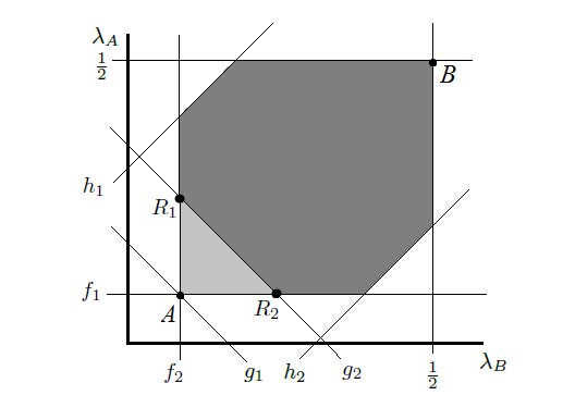
Minimising the QMI reduces to finding the minimum of the classical binary entropy sum $H(\lambda_{A})+H(\lambda_{B})$ over $\mathcal{R}$. It is not quite as simple as it may seem because the domain is not convex, see section VI.1. We first vary each of the terms in the sum separately. Concavity of the entropy (and symmetry about its maximum at $\lambda_{\mu}=\frac{1}{2}$) implies that $H(\lambda_{\mu})$ decreases as $\lambda_{\mu}$ tends to zero. The line that bounds $\mathcal{R}$ closest to zero is $g_{p}$: $\lambda_{A}+\lambda_{B}=\lambda_{2}+\lambda_{3}+2\lambda_{4}$ so the minimum of $H(\lambda_{A})+H(\lambda_{B})$ occurs somewhere on this boundary of $\mathcal{R}$. We show in Appendix A that the minimum of this function occurs at points $R_{1},R_{2}$ in figure 1 where

or vice versa, and the joint state (modulo the equivalence class of the QMI) which corresponds to it is

where $\lambda_{jk}$ is a reindexing of $\lambda_{i}$ ($\lambda_{00}=\lambda_{1},\lambda_{01}=\lambda_{2},\dots$) and $\{|e_{j}\rangle\},\{|f_{k}\rangle\}$ are qubit basis states for systems $A$ and $B$ respectively. The QMI for two qubits has a minimum value of

Here we have used the binary entropy notation: $H(\lambda_{3}+\lambda_{4})\equiv H(\lambda_{1}+\lambda_{2})\equiv H(\lambda_{1}+\lambda_{2},\lambda_{3}+\lambda_{4})$.

Any state $\rho=\sum_{i=1}^{4}\lambda_{i}|\psi_{i}\rangle\langle\psi_{i}|$ diagonal in the basis ${|\psi_{i}\rangle}$ along the unitary orbit of $\rho_{min}$ can be transformed to $\rho_{min}$ by the unitary $U_{min}=\sum_{i=1}^{4}|ef_{i}\rangle\langle\psi_{i}|$ where $|ef_{i}\rangle=|e_{j}\rangle|f_{k}\rangle$ are products of qubit basis states and $j,k=0,1$ are the binary representation of $i$.

So to answer the initial question, for a two-qubit system, the maximum that the QMI can change by over the domain of states in $\mathcal{O}_{\rho}$ with $\mathrm{spec}(\rho)=\{\lambda_{i}\}_{i=1}^{4}$, $\lambda_{i}\geq\lambda_{i+1}$, is

In this section we seek the maximum change in the QMI

subject to $\rho^{\prime}=U\rho U^{{\dagger}}$ where $U$ is now an energy-conserving unitary satisfying $E=\mbox{Tr}(\rho H)=\mbox{Tr}(\rho^{\prime}H)$. $H$ is a Hamiltonian for the composite system $AB$, taken to be local $H=H_{A}+H_{B}$, and the initial reduced states are thermal with respect to $H_{A},H_{B}$. These are the assumptions for the heat flow model between two quantum systems, Example 2 in Ref. [2]. Below we find the maximum $\Delta I_{E}$ when A and B are qubits.

We take the local Hamiltonians $H_{A},H_{B}$ of the initial subsystem states to be equal ²² 2 The following results also hold when $H_{A}=UH_{B}U^{{\dagger}}$ but not if the energy spacings between the ground and excited levels differ. The reason (c.f. Appendix B) is that this defines an energy conserving region that is bounded by a skewed line, it is of the form $a\lambda_{A}+b\lambda_{B}=C$, where $a\neq b$ and $C$ is a constant, and the maximally correlated state is no longer at the point where $\lambda_{A}=\lambda_{B}$.: the ground and excited states energies are zero and one respectively and the energy eigenbasis is the computational basis $\{|0\rangle,|1\rangle\}$ thus $H_{\mu}=|1\rangle\langle 1|_{\mu}$. We can write the initial (thermal) reduced state of $\rho$ as

where $\lambda^{i}_{\mu}=e^{-1/T_{\mu}}/\mbox{Tr}(\rho_{\mu})\leq\frac{1}{2}$ and $T_{\mu}$ is the temperature of system $\mu$.

Let us suppose that during the energy exchange interaction (a global energy conserving unitary on $\rho$) correlations decrease, i.e. the two systems $A,B$, though locally thermal, are initially correlated. We would therefore like to minimise $S(\rho^{\prime}_{A})+S(\rho^{\prime}_{B})$ subject to total average energy conservation. The initial total energy set by the initial state $\rho$ is

with $0\leq E\leq 1$.

Note: The point $(\lambda^{i}_{A},\lambda^{i}_{B})\in\mathcal{R}$ is on the line $\lambda_{A}+\lambda_{B}=E$, the thick black line in figure 2 (d). The joint states represented by this line all have total energy $E$ and their reduced states are thermal. The QMI, or equivalently just $H(\lambda_{A})+H(\lambda_{B})$, is concave on this line, which is easily seen when the function is written as $H(\lambda_{A})+H(E-\lambda_{A})$, and its maximum occurs when $\lambda_{A}=\lambda_{B}=\frac{E}{2}$, point q in the figure. Hence the maximum possible initial value of the QMI for a state with total average $E$ is $2H(\frac{E}{2})$.

After the global unitary transformation $U\rho U^{{\dagger}}=\rho^{\prime}$, the local subsystem states evolve to $\rho^{\prime}_{\mu}=(1-\lambda^{\prime}_{\mu})|v\rangle_{\mu}\langle v|_{\mu}+\lambda^{\prime}_{\mu}|\bar{v}\rangle_{\mu}\langle\bar{v}|_{\mu}$ with $\lambda^{\prime}_{\mu}\leq\frac{1}{2}$ and $\{|v\rangle_{\mu},|\bar{v}\rangle_{\mu}\}$ is a qubit basis

The final total average energy $E^{\prime}=\mbox{Tr}(\rho^{\prime}_{A}H_{A})+\mbox{Tr}(\rho^{\prime}_{B}H_{B})$ ($\rho_{A},\rho_{B}$ are not constrained to being diagonal in $H_{A},H_{B}$) is

In order for energy to be conserved, $E^{\prime}=E$. This condition and equation (15) gives a collection of straight lines, defining a region $\mathcal{R}_{E}\subseteq\mathcal{R}$ representing joint states which could have total energy $E$ for some choice of angles $\theta_{A},\theta_{B}$.

$\mathcal{R}_{E}$ is given by $\lambda_{A}+\lambda_{B}\leq E$, for the derivation see Appendix B and for a visualisation see figure 2 (d). The energy conserving region always contains the minimally correlated state, hence the greatest possible change in the QMI at constant average energy $E$ occurs when the initial state occurs when $\lambda^{i}_{A}=\lambda^{i}_{B}=\frac{E}{2}$ (these marginals could define multiple global states, even after factoring out the states in the equivalence class of the QMI, see section IV.1) and the final state is the minimally correlated one, $\rho_{min}$ given by equation (9), with $\theta_{A},\theta_{B}$ chosen such that equation (15) is satisfied (there is a range of angles which do this). We have then that

The way to think about the region $\mathcal{R}_{E}$ intuitively is that it contains final states whose marginals in general have longer Bloch vectors than the initial $\rho$, achieving this higher local purity is made possible by using up the correlations in the joint state. The constant energy condition is met by rotating the Bloch vectors off the energy axis by the angles $\theta_{A},\theta_{B}$, thereby adding coherence what was originally a thermal state.

Note that if we insist the also the final states are thermal, then the energy conserving region is just the set of states in $\mathcal{R}$ that are on the line $\lambda_{A}+\lambda_{B}=E$. The maximally correlated state is then still at $\lambda_{A}=\lambda_{B}=\frac{E}{2}$ but the minimally correlated one is at the edge of the line.

A two qubit density matrix is specified by 15 parameters, a point in $\mathcal{R}$ defines only 5 independent parameters $(\lambda_{A},\lambda_{B},\lambda_{1},\lambda_{2},\lambda_{3})$, hence there is a lot of degeneracy as each point in $\mathcal{R}$ corresponds to a whole set of compatible joint states. Modulo the parameters that don’t affect the QMI (the directions of the Bloch vectors, which requires 4 more parameters) there are still 6 parameters that can be freely chosen. In appendix A we show that the coordinate in $\mathcal{R}$ that represents $\rho_{min}$ is given by a unique state (modulo local unitaries and swaps). However there are points in $\mathcal{R}$ for which this is not true, these points determine states that have the same QMI but are not related by local unitaries or swaps, hence they would have different amounts of correlation, or entanglement, if we used another measure that, say, depended on the correlation- or T-matrix of the state, whose elements are $t_{ij}=\mbox{Tr}(\sigma^{i}\otimes\sigma^{j}\rho)$, $i,j=1,2,3$ and $\sigma^{i}$ is a Pauli matrix. We illustrate this with an example of a “triple point” in $\mathcal{R}(\Lambda)$. Defining

where the matrix is written in the computational basis, three states that correspond to the same $\lambda_{A},\lambda_{B}$ but are not connected by a symmetry of the QMI are $\rho(\lambda_{1},\lambda_{2},\lambda_{3},\lambda_{4},\frac{1}{\sqrt{2}},\frac{\lambda_{3}-\lambda_{4}}{\lambda_{1}-\lambda_{4}})$, $\rho(\lambda_{2},\lambda_{1},\lambda_{3},\lambda_{4},0,\frac{\lambda_{3}-\lambda_{4}}{\lambda_{2}-\lambda_{4}})$, $\rho(\lambda_{3},\lambda_{1},\lambda_{2},\lambda_{4},0,1)$ and

We know also of “double points” and correspondingly $\rho_{min}$ is a “single point”, shown in Appendix A.

Despite the value of the QMI not being sensitive to these different states, their dynamics under energy conserving unitaries leads to different values of $\Delta I$, and it is precisely the change in QMI which is the physically relevant quantity, see Ref. [2]: it is in this way that these hidden correlations are revealed.

There are many ways in which we could analyse the effect of a global unitary on a two qubit state, with regards to its position in $\mathcal{R}$. To simplify the task, we concentrate on some “elementary” transformations only rotating in two-dimensional subspaces and discuss what their consequences are for energy conservation.

Let us assume that the local bases are fixed in the computational basis, then the individual and total Hamiltonians are $H_{A}=H_{B}=|1\rangle\langle 1|,H=H_{A}\otimes\mathbb{I}+\mathbb{I}\otimes H_{B}=|01\rangle\langle 01|+|10\rangle\langle 10|+2|11\rangle\langle 11|$. There are two key unitary transformations (matrices are all written in the computational basis) that are effective two-dimensional rotations:

where the interaction Hamiltonians are $H^{(o)}=\frac{1}{2}(X\otimes Y-Y\otimes X)$ and $H^{(e)}=-\frac{1}{2}(X\otimes Y+Y\otimes X)$, $X,Y$ are Pauli matrices. Since $[H^{(o)},H]=0$, $U^{(o)}$ is a strong energy conserving unitary (SECU). In terms of its action on the reduced state eigenvalues (and therefore on the QMI when starting from states that are locally diagonal in $H_{A},H_{B}$ which is all that we require, see example 2 in Ref. [2]) it is the most general unitary that commutes with the total Hamiltonian.

The matrix $U^{(o)}(\theta)$ rotates in the energy degenerate “odd” subspace $\{|01\rangle,|10\rangle\}$ and $U^{(e)}(\phi)$ rotates in the “even” subspace $\{|00\rangle,|11\rangle\}$, but is not energy conserving. $U^{(o)}(\theta)$ and $U^{(e)}(\phi)$ commute. Let the initial state be diagonal in the computational basis

and the elements on the diagonal are some permutation of eigenvalues $\Lambda=\{\lambda_{i}\}_{i=1}^{4}$. To see how the unitaries transform $\rho_{0}$ in the region $\mathcal{R}$ we need to look at the (lowest) eigenvalue of the reduced states. A state evolved under these unitaries looks like $\rho(\alpha,\beta,\gamma,\delta,\cos\theta,\cos\phi)$ in equation (IV.1), it is often called an “X-state”. Note that $\rho(\alpha,\beta,\gamma,\delta,\cos\theta,\cos\phi)$ has reduced states that are diagonal in the local bases $H_{A},H_{B}$, that is, its local states are thermal (the spectrum can be equated to a Gibbs distribution). In this notation $\rho_{0}=\rho(\alpha,\beta,\gamma,\delta,1,1)$.

The reduced state eigenvalues of $\rho(\alpha,\beta,\gamma,\delta,\cos\theta,\cos\phi)$ are

if we pick $\min\{\alpha-\delta,\beta-\gamma\}=\beta-\gamma$. Care must be taken to ensure that these eigenvalues are the smallest depending on the ordering used for $\alpha,\beta,\gamma,\delta$.

Following from this, $\lambda_{A}+\lambda_{B}=1-(\alpha-\delta)\cos\phi$, hence varying $\phi$ provides a set of lines of the form $\lambda_{A}+\lambda_{B}=C_{1}$. On the other hand, $\lambda_{B}-\lambda_{A}=(\beta-\gamma)\cos\theta$, thus $\theta$ defines the lines $\lambda_{A}=\lambda_{B}+C_{2}$. Therefore, when the initial state is that given in equation (IV.2), we can describe the evolution of the odd and even unitaries fairly simply in terms of the marginals and the regions that they trace out in $\mathcal{R}$. It is easy also to see their effect on the QMI (in simplified notation):

where $a,b,c,m,n$ are all constants related to terms in equations (38) and (39), and the QMI is (separately) concave over the domains $x$ and $y$.

It is shown in section VI.4 that of the $4!$ possible orderings of $\lambda_{i}$, $i=1,2,3,4$, there are only three classes of permutations which give distinct values of the QMI. Representative states for each class are taken to be $\tau^{(1)}=\rho(\lambda_{1},\lambda_{2},\lambda_{3},\lambda_{4},1,1)$, $\tau^{(2)}=\rho(\lambda_{2},\lambda_{1},\lambda_{3},\lambda_{4},1,1)$, $\tau^{(3)}=\rho(\lambda_{3},\lambda_{1},\lambda_{2},\lambda_{4},1,1)$. Note again that, especially when calculating energies, care must be taken so that the reduced states of each of these are in the form $\rho_{\mu}=(1-\lambda_{\mu})|0\rangle\langle 0|+\lambda_{\mu}|1\rangle\langle 1|$ with $0\leq\lambda_{\mu}\leq\frac{1}{2}$ - local unitaries may be used to ensure this condition. Using each of these as an initial state $\rho_{0}$, figure 3 depicts the effect of $U^{(e)},U^{(o)}$ on the each of their marginals.

We can clearly see the triple point described in section IV.1, labelled TP in figure 3, as well as many other overlaps corresponding to triple and double points. A corollary of this is that starting at a triple/double point, the unitary $U^{(o)}$ generates portions of the line $\lambda_{A}+\lambda_{B}=C_{1}$ that are of varying length, depending on which exact state we started with. The longer the length, the lower the correlations can go since the QMI is concave on the line.

Comparing figure 3 with the full allowed region $\mathcal{R}(\Lambda)$, see for instance figure 2 (d), we see that just these two unitaries can evolve the classically correlated state to almost every point in $\mathcal{R}(\Lambda)$. The “wings” that are missing in figure 3 can be obtained using one more unitary

with $\tilde{H}=-\frac{1}{2}(\mathbb{I}\otimes Y+Z\otimes Y)$. This unitary acting on $\rho(\lambda_{1},\lambda_{2},\lambda_{3},\lambda_{4},\cos\theta,1)$ results in figure 4. By considering the transformation this unitary generates on the marginal eigenvalues, it is simple to show that these three unitaries generate all points in $\mathcal{R}$. To summarise, we have identified how to reach all points in the allowed region $\mathcal{R}$ starting from classically correlated states using just three unitaries, overlaps are easily seen to be double/triple points and the joint state they correspond to is known.

Let us take a closer look at unitary evolution for states in the energy conserving region $\mathcal{R}_{E}\subseteq\mathcal{R}$, defined as the set fulfilling $\lambda_{A}+\lambda_{B}\leq E$. We set the initial state now as the maximally correlated state for this subregion $\rho_{0}=\rho_{E}^{max}$, it is at the point on the line $\lambda_{A}+\lambda_{B}=E$ where $\lambda_{A}=\lambda_{B}$. The local and total Hamiltonians are still the same (diagonal in the computational basis). To conserve energy, the unitary evolution of $\rho_{0}$ must obey

There are two types of unitary that satisfy this: SECUs $U_{S}$ that commute with the total Hamiltonian (above we stated that the only SECU for this Hamiltonian is $U^{(o)}$) and weak energy conserving unitaries (WECUs) $U_{W}$ that do not commute with the total Hamiltonian but preserve the total energy on average.

Depending on the exact form of $\rho_{E}^{max}$ (could be e.g. a triple point) the SECU evolves it along some portion of the line $\lambda_{A}+\lambda_{B}=E$. Getting to other states in the region $\mathcal{R}_{E}$, for instance where $\lambda_{A}+\lambda_{B}<E$, and conforming with the energy conserving condition, equation (15), requires WECUs, which can shrink $\lambda_{A},\lambda_{B}$, and local unitaries to rotate the local bases by appropriate angles $\theta_{A},\theta_{B}$. This generally amounts to elongating the local Bloch vectors and rotating them off the energy axis in order to preserve total average energy. Consequently, the reduced states are permitted to be non-diagonal in the energy eigenbasis and so they are no longer thermal, however we argue in Ref. [2] and the next section that this is still physically and thermodynamically relevant. Note there is a range of angles $\theta_{A},\theta_{B}$ that satisfy equation (15) and the amount energy exchanged between the qubits depends on these angles.

There is an interesting conclusion to be noted from all of this: sometimes a SECU can only transform a state with total energy $E$ along a portion of the line $\lambda_{A}+\lambda_{B}=E$ but there are states that are on $\lambda_{A}+\lambda_{B}=E$ in $\mathcal{R}$ that are not reachable by the SECU and these unreachable states are locally thermal. This means that a WECU is required to get to these states. Hence if we, say, restricted our heat flow model (in the next section) to initial and final states being thermal, with total energy conserved, it would not be general enough to only consider SECUs, one would still have to include the WECUs for the full analysis.

Another property of transformations under unitaries that commute with the Hamiltonian is that the quantum variance $\delta=\mbox{Tr}[\rho H^{2}]-(\mbox{Tr}[\rho H])^{2}$ remains constant as $\rho\rightarrow U_{S}(t)\rho U_{S}(t)^{{\dagger}}$. We assume constant average energy $\mbox{Tr}[\rho H]=E$ so changes in $\delta$ only depend on the first term. All moments of $H$, $\mbox{Tr}[\rho H^{k}]$ for $k=1,2...$ are constant for SECUs. This means that the statistics of all the measurements of the energy of $U_{S}(t)\rho U_{S}(t)^{{\dagger}}$ will be the same, due to total constant energy and the reduced states being diagonal in the energy eigenbasis. Quantum uncertainty due to coherence is introduced when the observable and the state are not locally codiagonal, and in general the term $\mbox{Tr}[\rho H^{2}]$ will increase for unitaries the do not commute with $H$.

The model for the heat flow, example 2 in Ref. [2], between two systems $A$ and $B$ is based on three assumptions: (1) the global evolution of the composite system $\rho$ is unitary $\rho\rightarrow\rho^{\prime}=U\rho U^{{\dagger}}$, (2) the total average energy of $\rho$ is conserved, $E=\mbox{Tr}(\rho H)=\mbox{Tr}(\rho^{\prime}H)$ ³³ 3 The total Hamiltonian is local $H=H_{A}+H_{B}$ and $H_{A},H_{B}$ are Hamiltonians for the reduced states of $\rho$ but not necessarily of $\rho^{\prime}$. and (3) the reduced states $\rho_{A},\rho_{B}$ of the initial state $\rho$ are thermal.

This model places a limit on the amount of heat that can flow from one system to another. It adheres to conditions (1)-(3) above and, using the fact that the free energy is minimised by a thermal state, yields the inequality [2]

where $Q_{A}$ is the heat into system A, $T_{A}$ $(T_{B})$ is the initial temperature of system A (B), $k$ is the Boltzmann constant and $\Delta I_{\mathrm{heat}}$ is the difference in the mutual information before and after the heat exchange interaction, its greatest value for two qubits is displayed in equation (16), $|\Delta I_{\mathrm{heat}}|\leq\Delta I_{E}$.

To reduce misconceptions, we would like to discuss several key points about the physical assumptions underlying the application of our formal results to physical scenarios involving closed quantum systems. We use the heat flow model as a base for our discussion, but bear in mind that it is not limited to this one situation, nor is it restricted to qubit systems.

In an attempt to explain equilibration between two systems, Partovi [17] devised a collision model between two particles. We outlined its principles in example 3 in Ref. [2] and claimed that when the two systems are qubits, one of Partovi’s restrictions can be weakened. Here we elaborate on why this is true and furthermore we explain why in the higher dimensional case, Partovi’s initial assumptions must hold.

The fundamentals of the collision process is summarised here: initially the two systems are described by a joint product state $\rho$, they interact via a global energy conserving unitary and then they decorrelate, forgetting any correlations that are produced and rendering the process irreversible (this moves the system to a new unitary orbit). More compactly: $\rho=\rho_{A}\otimes\rho_{B}\rightarrow\rho^{\prime}=U\rho U^{{\dagger}}\rightarrow\rho^{\prime}_{A}\otimes\rho^{\prime}_{B}$. At the end of these steps, the local entropies and global entropy has increased, $\Delta S_{A}+\Delta S_{B}\geq 0$, $\Delta S\geq 0$. This whole procedure is then reiterated until the entropies are maximised and the systems reach equilibrium.

We propose a modified version of the model where, instead of the systems completely decorrelating after the unitary interaction, the joint state of the system dephases to a classically correlated state by losing its “off-diagonal” components (again this process transfers the system to a new unitary orbit). Note that this requires the introduction of local bases. This process may be more physically meaningful because dephasing occurs faster than decorrelation in real systems.

Let $\sigma,\sigma^{\prime}$ be two minimum QMI states on some unitary orbits. Then does the process $\sigma\rightarrow\rho^{\prime}=U\sigma U^{{\dagger}}\rightarrow\sigma^{\prime}$ achieve the same entropic increase as the original Partovi scheme? $\sigma^{\prime}$ is the dephased $\rho^{\prime}$.

References

- [1] E. Schrödinger, Phys. Rev. 28, 10491070 (1926).
- [2] S. Jevtic, D. Jennings, and T. Rudolph, Phys. Rev. Lett. 108, 110403 (2012).
- [3] G. McConnell and D. Jennings, arXiv:1205.3517 [quant-ph] (2012).
- [4] K. Modi, arXiv:0902.0735 [quant-ph] (2009).
- [5] D. Sych and G. Leuchs, New J. Phys. 11, 013006 (2009).
- [6] A. Klyachko, arXiv:0409113 [quant-ph] (2004).
- [7] S. Bravyi, Quant. Inf. and Comp. 4, 012 (2004).
- [8] M. Christandl and G. Mitchison, Commun. Math. Phys. 261, 789797 (2006).
- [9] M. H. Partovi, Phys. Rev. E 77, 021110 (2008).
- [10] S. Popescu, T. Short, and A. Winter, Nature Phys. 2, 758 (2006).
- [11] A. E. Allahverdyan, R. Balian, and T. M. Nieuwenhuizen, EPL 67, 565 (2004).
- [12] M. Horodecki and J. Oppenheim, arXiv:1111.3834 [quant-ph] (2011).
- [13] H. Weimer, M. J. Henrich, F. Rempp, H. Schröder, and G. Mahler, EPL 83, 30008 (2008).
- [14] T. M. Nieuwenhuizen, J. Mod. Optics 50, 2433 (2003).
- [15] A. E. Allahverdyan and T. M. Nieuwenhuizen, J. Phys. A: Math. Gen. 36, 875 (2003).
- [16] E. H. Lieb and J. Yngvason, Phys. Rep. 310, 1 (1997).
- [17] M. H. Partovi, Phys. Lett. A 137, 440 (1989).
- [18] A. Wehrl, Rep. on Math. Phys. 6, 15 (1974).
- [19] A. W. Marshall, I. Olkin, and B. C. Arnold, Inequalities: Theory of Majorization and Its Applications (2009), 2nd ed.
- [20] J. S. Frame, G. de B. Robinson, and R. M. Thrall, Can. J. Math. 6, 316 (1954).
- [21] F. G. S. L. Brandão, M. Horodecki, J. Oppenheim, J. M. Renes, and R. W. Spekkens, arXiv:1111.3882 [quant-ph] (2011).