Higher-Order Momentum Distributions and Locally Affine LDDMM Registration
Abstract
To achieve sparse parametrizations that allows intuitive analysis, we aim to represent deformation with a basis containing interpretable elements, and we wish to use elements that have the description capacity to represent the deformation compactly. To accomplish this, we introduce in this paper higher-order momentum distributions in the LDDMM registration framework. While the zeroth order moments previously used in LDDMM only describe local displacement, the first-order momenta that are proposed here represent a basis that allows local description of affine transformations and subsequent compact description of non-translational movement in a globally non-rigid deformation. The resulting representation contains directly interpretable information from both mathematical and modeling perspectives. We develop the mathematical construction of the registration framework with higher-order momenta, we show the implications for sparse image registration and deformation description, and we provide examples of how the parametrization enables registration with a very low number of parameters. The capacity and interpretability of the parametrization using higher-order momenta lead to natural modeling of articulated movement, and the method promises to be useful for quantifying ventricle expansion and progressing atrophy during Alzheimer’s disease.
keywords
LDDMM, diffeomorphic registration, RHKS, kernels, momentum, computational anatomyAMS
65D18, 65K10, 41A151 Introduction
In many image registration applications, we wish to describe the deformation using as few parameters as possible and with a representation that allows intuitive analysis: we search for parametrizations with basis elements that have the capacity to describe deformation sparsely while being directly interpretable. For instance, we wish to use such a representation to compactly describe the progressive atrophy that occurs in the human brain suffering from Alzheimer’s disease and that can be detected by the expansion of the ventricles [19, 13].
Image registration algorithms often represent translational movement in a dense sampling of the image domain. Such approaches fail to satisfy the above goals: low dimensional deformations such as expansion of the ventricles will not be represented sparsely; the registration algorithm must optimize a large number of parameters; and the expansion cannot easily be interpreted from the registration result.
In this paper, we use higher-order momentum distributions in the LDDMM registration framework to obtain a deformation parametrization that increases the capacity of sparse approaches with a basis consisting of interpretable elements. We show how the higher-order representation model locally affine transformations, and we use the compact deformation description to register points and images using very few parameters. We illustrate how the deformation coded by the higher-order momenta can be directly interpreted and that it represents information directly useful in applications: with low numbers of control points, we can detect the expanding ventricles of the patient shown in Figure 1.


1.1 Background
Most of the methods for non-rigid registration in medical imaging model the displacement of each spatial position by either a combination of suitable basis functions for the displacement itself or for the velocity of the voxels. The number of control points vary between one for each voxel [2, 17, 7] and fewer with larger basis functions [25, 5, 11]. For all methods, the infinite-dimensional space of deformations is approximated by the finite- but high-dimensional subspace spanned by the parametrization of the individual method. The approximation will be good if the underlying deformation is close to this subspace, and the representation will be compact, if few basis functions describe the deformation well. The choice of basis functions play a crucial role, and we will in the rest of the paper denote them deformation atoms. Two main observations constitute the motivation for the work presented in this paper:
Observation 1: Order of the Deformation Model. In the majority of registration methods, the deformation atoms model the local translation of each point. We wish a richer representation which is in particular able to model locally linear components in addition to local translations. The Polyaffine and Log-Euclidean Polyaffine [3, 1] frameworks pursue this by representing the velocity of a path of deformations locally by matrix logarithms. Ideas from the Polyaffine methods have recently been incorporated in e.g. the Demons algorithm [32] but, to the best of our knowledge, not in the LDDMM registration framework. We wish to extend the set of deformation atoms used in LDDMM to allow representation of first- and higher-order structure and hence incorporate the benefits of the Polyaffine methods in the LDDMM framework.
Observation 2: Order of the Similarity Measure. When registering DT images, the reorientation is a function of the derivative of the warp; curve normals also contain directional information which is dependent on the warp derivative and airway trees contain directional information in the tree structure which can be used for measuring similarity. These are examples of similarity measures containing higher-order information. For the case of image registration, the warp derivative may also enter the equation either directly in the similarity measure [24, 22] or to allow use of more image information than provided by a sampling of the warp. Consider an image similarity measure on the form . A finite sampling of the domain can approximate this with
Letting be uniformly distributed points around , we can increase the amount of image information used in without additional sampling of the warp by using a first-order approximation of :
This can be considered an increase from zeroth to first-order
in the approximation of . Besides including more image information
than provided by the initial sampling of the warp, the increase in order allows capture of
non-translational information - e.g. rotation and dilation - in the similarity
measure. The approach can be seen as a specific case of similarity smoothing; more examples
of smoothing in intensity based image registration
can be found in [9].
We focus on deformation modeling with the Large Deformation Diffeomorphic Metric Mapping (LDDMM) registration framework which has the benefit of both providing good registrations and drawing strong theoretical links with Lie group theory and evolution equations in physical modeling [8, 34]. Most often, high-dimensional voxel-wise representations are used for LDDMM although recent interest in compact representations [11, 28] show that the number of parameters can be much reduced. These methods use interpolation of the velocity field by deformation atoms to represent translational movement but deformation by other parts of the affine group cannot be compactly represented.
The deformation atoms are called kernels in LDDMM. The kernels are centered at different spatial positions and parameters determine the contribution of each kernel. In this paper, we use the partial derivative reproducing property [35] to show that partial derivatives of kernels fit naturally in the LDDMM framework and constitute deformation atoms along with the original kernels. In particular, these deformation atoms have a singular higher-order momentum and the momentum stays singular when transported by the EPDiff evolution equations. We show how the higher-order momenta allow modeling locally affine deformations, and they hence extend the capacity of sparsely discretized LDDMM methods. In addition, they comprise the natural vehicle for incorporating first-order similarity measures in the framework.
1.2 Related Work
A number of methods for non-rigid registration have been developed during the last decades including non-linear elastic methods [21], parametrizations using static velocity fields [2, 17], the demons algorithm [29, 32], and spline-based methods [25, 5]. For the particular case of LDDMM, the groundbreaking work appeared with the deformable template model by Grenander [16] and the flow approach by Christensen et al. [7] together with the theoretical contributions of Dupuis et al. and Trouvé [10, 30]. Algorithms for computing optimal diffeomorphisms have been developed in [4], and [31] uses the momentum representation for statistics and develops a momentum based algorithm for the landmark matching problem.
Locally affine deformations can be modeled using the Polyaffine and Log-Euclidean Polyaffine [3, 1] frameworks. The velocity of a path of deformations is here computed using matrix logarithms, and the resulting diffeomorphism flowed forward by integrating the velocity. Ideas from the Polyaffine methods have recently been incorporated in e.g. the Demons algorithm [32, 26]. In LDDMM, the deformation atoms, the kernels, represent translational movement and the non-translational part of affine transformations cannot directly be represented. We will show how partial derivatives of kernels constitute deformation atoms which allow representing the linear parts of affine transformations. From a mathematical point of view, this is possible due to the partial derivative reproducing property (Zhou [35]). The partial derivative reproducing property, partial derivatives of kernels, and first-order momenta have previously been used in [6] to derive variations of flow equations for LDDMM DTI registration, in [14] to match landmarks with vector features, and in [15] to match surfaces with currents. Confer the monograph [34] for information on RKHSs and their role in LDDMM.
In order to reduce the dimensionality of the parametrization used in LDDMM, Durrleman et al. [11] introduced a control point formulation of the registration problem by choosing a finite set of control points and constraining the momentum to be concentrated as Dirac measures at the point trajectories. As we will see, higher-order momenta make a finite control point formulation possible which is different in important aspects. Younes [33] in addition considers evolution in constrained subspaces.
Higher-order momenta increase the capacity of the deformation parametrization, a goal which is also treated in sparse multi-scale methods such as the kernel bundle framework [28]. This method concerns the size of the kernel in contrast to the order which we deal with here. As we will discuss in the experiments section, the size of the kernel is important when using the higher-order representation as well, and representations using higher-order momenta will likely complement the kernel bundle method if applied together.
1.3 Content and Outline
We start the paper with an overview of LDDMM registration and the mathematical constructs behind the method. In the following section, we describe registration using higher-order image information and parameterization using higher-order momentum distributions. We then turn to the mathematical background of the method and describe the evolution of the momentum and velocity fields governed by the EPDiff evolution equations in the first-order case. The next sections describes the relation to polyaffine approaches, the effect of varying the initial conditions, and the backwards gradient transport. We then provide examples and illustrate how the deformation represented by first-order atoms can be interpreted when registering human brains with progressing atrophy. The paper ends with concluding remarks and outlook.
2 LDDMM Registration, Kernels, and Evolution Equations
In the LDDMM framework, registration is performed through the action of diffeomorphisms on geometric objects. This approach is very general and allows the framework to be applied to both landmarks, curves, surfaces, images, and tensors. In the case of images, the action of a diffeomorphism on the image takes the form , and given a fixed image and moving image , the registration amounts to a search for such that . In exact matching, we wish be exactly equal to but, more frequently, we allow some amount of inexactness to account for noise in the images and allow for smoother diffeomorphisms. This is done by defining a similarity measure on images and a regularization measure to give a combined energy
| (1) |
Here is a positive real representing the trade-off between regularity and goodness of fit. The similarity measure is in the simplest form the -error but more advanced measures can be used (e.g. [23, 18, 9]).
In order to define the regularization term , we introduce some notations in the following: Let the domain be a subset of with , and let denote a Hilbert space of vector fields such that with associated norm is included in and admissible [34, Chap. 9], i.e. sufficiently smooth. Given a time-dependent vector field with
| (2) |
the associated differential equation has with initial condition a diffeomorphism as unique solution at time . The set of diffeomorphisms built from by such differential equations is a Lie group, and is its tangent space at the identity. Using the group structure, is isomorphic to the tangent space at each point . The inner product on associated to a norm makes a Riemannian manifold with right-invariant metric. Setting , the map is a path from to with energy given by (2) and generated by . We will use this notation extensively in the following. A critical path for the energy (2) is a geodesic on , and the regularization term is defined using the energy by
| (3) |
i.e. it measures the minimal energy of diffeomorphism paths from to . Since the energy is high for paths with great variation, the term penalizes highly varying paths, and a low value of thus implies that is regular.
2.1 Kernel and Momentum
As a consequence of the assumed admissibility of , the evaluation functionals is well-defined and continuous for any . Thus, for any the map belongs to the topological dual , i.e. the continuous linear maps on . This in turn implies the existence of spatially dependent matrices , the kernel, such that, for any constant vector , the vector field represents and for any , point and vector . This latter property is denoted the reproducing property and gives the structure of a reproducing kernel Hilbert space (RKHS). Tightly connected to the norm and kernels is the notion of momentum given by the linear momentum operator which satisfies
for all . The momentum operator connects the inner product on with the inner product in , and the image of an element is denoted the momentum of . The momentum might be singular and in fact is the Dirac measure . Considering as the map , can be viewed as the inverse of . We will use the symbol for the momentum when considered as a functional in while we switch to the symbol when the momentum is realized as a vector field on or for the parameters when the momentum consists of a finite number of singular point measures.
Instead of deriving the kernel from , the opposite approach can be used: build from a kernel, and hence impose the regularization in the framework from the kernel. With this approach, the kernel is often chosen to ensure rotational and translational invariance [34] and the scalar Gaussian kernel is an often used choice. Confer [12] for details on the construction of from Gaussian kernels.
2.2 Optimal Paths: The EPDiff Evolution Equations
The relation between norm and momentum leads to convenient equations for minimizers of the energy (1). In particular, the EPDiff equations for the evolution of the momentum for optimal paths assert that if is a path minimizing with minimizing and is the derivative of then satisfies the system
with and denoting spatial differentiation of the momentum and velocity fields, respectively. The first equation connects the momentum with the velocity , and the second equation describes the time evolution of the momentum. In the most general form, the EPDiff equations describe the evolution of the momentum using the adjoint map. Following [34], define the adjoint for . The dual of the adjoint is the functional on the dual of defined by .11 1 Here and in the following, we will use the notation for evaluation of the functional on the vector field . Define in addition which then satisfies , and let denote the gradient of the similarity measure with respect to the inner product on so that for any variation and diffeomorphism path with derivative . For optimal paths , the EPDiff equations assert that with which leads to the conservation of momentum property for optimal paths. Conversely, the EPDiff equations reduce to simpler forms for certain objects. For landmarks , the momentum will be concentrated at point trajectories as Dirac measures leading to the finite dimensional system of ODE’s
| (4) |
3 Registration with Higher-Order Information
We here introduce higher-order momentum distributions for registration using
higher-order information with the LDDMM framework. We start by
motivating the construction by considering the approximation used when computing the similarity
measure. We then describe the deformation encoded by higher-order momenta and the evolution equations
in the finite case, and we use this to derive a registration algorithm using first-order information. The
mathematical background behind the method will be presented in the following
sections.
We will motivate the introduction of higher-order momenta by considering a specific case of image registration: we take on the goal of using a control point formulation [11] when solving the registration problem (1) and hence aim for using a relatively sparse sampling of the velocity or momentum field. To achieve this, we will consider the coupling between the transported control points and the similarity measure in order to ensure the momentum stays singular and localized at the point trajectories while removing the need for warping the entire image at every iteration of the optimization process.
Considering a similarity measure as discussed in the introduction, and a finite discretization with a sparse set of control points . While using to drive registration of the images will be very efficient in evaluating the warp in few points, it will suffer correspondingly from only using image information present in those points. Apart from not being robust under the presence of noise in the images, the discretization implies that local dilation or rotation around the points cannot be detected: any variation of keeping constant for all will not change . Formally, if is a diffeomorphism path that is equal to at and has derivative at , i.e. and , then
which vanishes if . Here denotes the derivative of with respect to the first variable.
A simple way to include more image information in the similarity measure is to convolve with a kernel , and thus extend to
with a normalization constant. If is a box kernel, this amounts to a finer sampling of both the image and warp, and hence a finer discretization of the Riemann integral. The kernel should not be confused with the RKHS kernel connected to the norm on that is used when generating the -gradient. A Gaussian kernel may be used for , and more information on using smoothing kernels for intensity based image registration can be found in [9, 36].
The measure is problematic since a variation of would affect not only the point but also , and will therefore be dependent on for any where is non-zero. In this situation, the momentum is no longer concentrated in Dirac measures located at , and it will be necessary to increase the sampling of the warp. However, a first-order expansion of yields the approximation
| (5) |
The measure is now again local depending only on and the first-order derivatives . It offers the stability provided by the convolution with , and, importantly, variations of keeping constant but changing do indeed affect the similarity measure. This implies that is able to catch rotations and dilations and drive the search for optimal accordingly. Please note the differences with the approach of Durrleman et al. [11]: when using as outlined here, the need for flowing the entire moving image forward is removed and the momentum field will stay singular directly thus removing the need for constraining the form of the velocity field.
3.1 Evolution and Deformation with Higher-Order Information
The dependence on in the similarity measure raises the question of how to represent variations of in the LDDMM framework. As we will outline here, higher-order momenta appear as the natural choice for such a representation that keeps the benefits of the finite control point formulation. Mathematical details will follow in the next sections.
Recall the reproducing property of the RKHS structure, i.e. for , and . Let us define the maps that extend the Diracs by measuring the derivative of at . These will be denoted higher-order Diracs, and we say that the momentum distribution is of higher-order if it is a sum of higher order Diracs. When applying the momentum operator to the higher-order Diracs, we will get partial derivatives of the RHKS kernel .
In particular, we will see that when using similarity measures such as , the momentum field will be a linear combination of higher-order Diracs and the velocity field will, correspondingly, be a linear combination of partial derivatives of . This will imply that the finite dimensional system of ODE’s (4) describing the EPDiff equations in the landmark case will be extended so that the velocity will contain partial derivatives . In the first-order case, we will get the velocity
| (6) |
where denotes the coefficients of the Dirac measures as in (4) but now the additional vectors denote the coefficients of the first-order Diracs for each of the dimensions . We will later show how these coefficients evolve. Combined with knowledge of how variations of and affect the system, we can transport variational information along the optimal paths specified by the EPDiff equations and thus provide the necessary building blocks for a first-order registration algorithm.
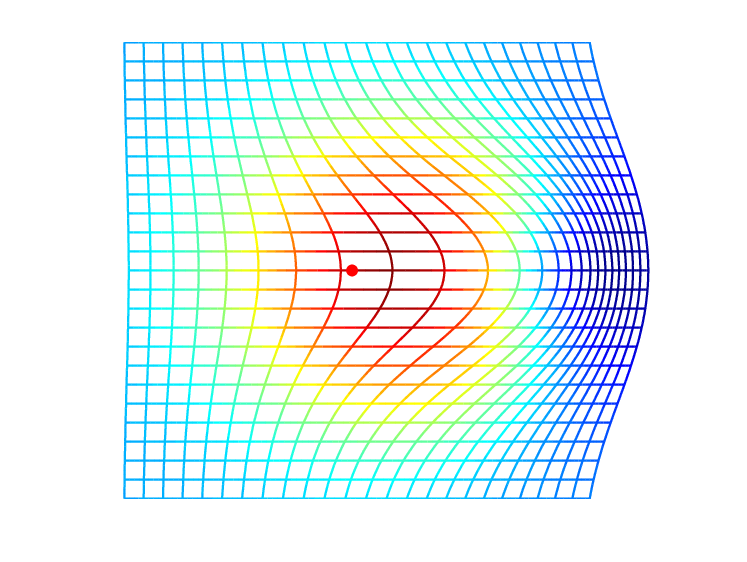
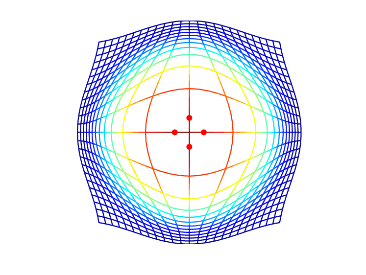
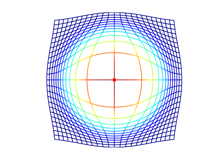
Figure 2 illustrates how the local translation encoded by the kernel is complemented by locally affine deformation when incorporating first-order momenta and corresponding partial derivatives of the kernel. Using the language of deformation atoms, the first-order constructions adds partial derivatives of kernels to the usual set of atoms, and the deformation atoms are thus able to compactly encode expansion, contraction, rotation etc. We can directly interpret the coefficients of the first-order momenta as controlling the magnitude of these first-order deformations. In Figure 3 in the experiments section, we give additional illustrations of the deformation encoded by the new atoms.
3.2 Algorithm for First-Order Registration
In this section, we will derive a registration algorithm for similarity measures incorporating first-order information such as . Since the algorithm works for general first-order measures, we will again let denote the similarity measure with being just a particular example.
There exists various choices of optimization algorithms for LDDMM registration. Roughly, they can be divided into two groups based on whether they represent the initial momentum/velocity or the entire path . Here, we take the approach of incorporating first-order momenta with the shooting method of e.g. Vaillant et al. [31]. The algorithm will take a guess for the initial momentum, integrate the EPDiff equations forward, compute the similarity measure gradient , and flow the gradient backwards to provide an improved guess.
The registration problem (1) consists of both the similarity measure and the minimal path energy . For e.g. landmark based registration, the similarity is most often expressed in terms of directly whether as the similarity measure is usually dependent on the inverse for image registration. In the first case, the gradient is known, and, given the initial momentum , we can obtain the gradient for a gradient descent based optimisation procedure from the backwards transport equations that we derive in Section 6. For the energy part, it is a fundamental property of critical paths in the LDDMM framework that the energy stays constant along the path. Thus, we can easily compute the gradient from the expressions provided in Section 4. Given this, the zeroth order matching algorithm in the initial momentum is generalized to zeroth and first-order momenta in Algorithm 1.
Traditionally, the similarity measure is in image matching formulated using the inverse of , and this approach was taken when formulating the approximation in (5). For this reason, at finite control point formulation is naturally expressed using a sampling in the target image with the algorithm optimizing for the momentum at time . The evaluation points are then generated by flowing backwards from to , and the gradient of can be computed in before being flowed forwards to update . Algorithm 1 will accommodate this situation by just reversing the integration directions. The control points can be chosen either at e.g. anatomically important locations, at random, or on a regular grid. In the experiments, we will register expanding ventricles using control points placed in the ventricles.
3.3 Numerical Integration
The integration of the flow equations can be performed with standard Runge-Kutta integrators such as Matlabs ode45 procedure. With zeroth order momenta only and points, the forward and backwards system consist of equations. With zeroth and first-order momenta, the forward system is extended to and the backwards system to . For , this implies an times increase in the size of the forward system and times increase in the backwards system. As suggested in Figure 2, the first-order system can be approximated using ensembles of zeroth-order atoms. Such an approximation would for require at least four zeroth-order atoms for each first-order atom making the size of the approximating system equivalent to the first-order system. Due to the non-linearity of the systems, the effect of the approximation introduced with such as an approach is not presently established.
In addition to the increase in the size of the systems, the extra floating point operations necessary for computing the more complicated evolution equations should be considered. The additional computational effort should, however, be viewed against the fact that the finite dimensional system can contain orders of magnitude fewer control points, and the added capacity of deformation description included in the derivative information. In addition and in contrast to previous approaches, we transport the similarity gradient only at the control point trajectories, again an order of magnitude reduction of transported information.
4 Higher-Order Momentum Distributions
We now link partial derivatives of kernels to higher-order momenta using the derivative reproducing property, and we provide details on the EPDiff evolution equations that we outlined in the previous section. We underline that the analytical of structure of LDDMM is not changed when incorporating higher-order momenta, and the evolution equations will thus be particular instances of the general EPDiff equations. These equations in Hamiltonian form constitutes the explicit expressions that allows implementation of the registration algorithm.
We will restrict to scalar kernels when appropriate for simplifying the notation. Scalar kernels are diagonal matrices where all diagonal elements are equal. Thus, we can consider both a matrix and a scalar so that the entries of the kernel in matrix form equals the scalar if and only if and otherwise.
4.1 Derivative Reproducing Property
Recall the reproducing property of the RKHS structure, i.e. for , and . Zhou [35] shows that this property holds not only for the kernel but also for its partial derivatives. Letting denote the derivative of at with respect to the multi-index ,
and defining for , Zhou proves that and that the partial derivative reproducing property
| (7) |
holds when the maps in are sufficiently smooth for the derivatives to exist. We denote the maps defined by higher-order Diracs, and we say that the momentum distribution is of higher order if it is a sum of higher-order Diracs. It follows that
As a consequence, we can connect higher-order momenta and partial derivatives of the kernel. Recall that the momentum map satisfies . With the higher-order momenta,
Thus or, shorter, . That is, partial derivatives of the kernel and higher-order momenta corresponds just as the kernels and Diracs measures in the usual RKHS sense.
Consider a map on diffeomorphisms e.g. an image similarity measure dependent on . In a finite dimensional setting with evaluation points , would decompose as with and . Introducing higher-order momenta, we let with multi-indices , and decompose as with . We allow to be empty and hence incorporate the standard zeroth order case. The partial derivative reproducing property now lets us compute the -gradient of as a sum of partial derivatives of the kernel.
Proposition 1.
Let denote the gradient with respect to the variable indexed by in the expression for . Then the gradient of with respect to the inner product in is given by .
Proof.
4.2 Momentum and Energy
As a result of Proposition 1, the momentum of the gradient of is . In general, if is represented by a sum of higher-order momenta, the energy can be computed using (7) as a sum of partial derivatives of the kernel evaluated at the points . To keep the notation brief, we restrict to sums of zeroth and first-order momenta in the following. If we get the energy
| (8) |
with denoting differentiation with the respect to the th variable, , and th coordinate, . For scalar symmetric kernels, this expression reduces to
4.3 EPDiff Equations
It is important to note that higher-order momenta offer a convenient representation for the gradients of maps incorporating derivative information but since the partial derivatives of kernels are members of and the higher order momentum in the dual , the analytical of structure of LDDMM is not changed. In particular, the adjoint form of the EPDiff equations, i.e. that optimal paths satisfy with , is still valid. The momentum is transported to the momentum by . Because
if is a sum of higher-order Diracs, will be sum of higher-order Diracs for all . However, since the time evolution of with the above relation involves derivatives of , this form is inconvenient for computing . Instead, we make use of the Hamiltonian form of the EPDiff equations [34, P. 265]. Here, the momentum is pulled back to but with a coordinate change of the evaluation vector field: the Hamiltonian form is defined by where the subscript stresses that is evaluated as a -dependent vector field. To simplify the notation, we write just instead of . Using this notation, the evolution equations become
| (9) |
The system forms an ordinary differential equation describing the evolution of the path and momentum [34] when does not involve derivatives of , e.g. when and hence is a vector field and the first equation therefore is an integral
For the higher-order case, we will need to incorporate additional information in the system.
Again we restrict to finite sums of zeroth and first-order point measures, and we therefore work with initial momenta on the form
| (10) |
with as usual denoting the point positions at time . Then
showing that with
| (11) |
The momentum can the be recovered as
and hence the coefficients of the momentum and (confer (10)) are given by and . We note that both and are coordinate vectors of the first-order parts of the momentum in ordinary and Hamiltonian form respectively. For each point and time , these coordinate vectors thus represent two tensors.
4.4 Time Evolution
Even though in (11) depend on the second order derivative of , we will show that the complete evolution in the zeroth and first-order case can be determined by solving for the points , the matrices , and the vectors . This will provide the computational representation we will use when implementing the systems.
It is shown in [34] that the evolution of the matrix is governed by
Inserting the Hamiltonian form of the higher-order momentum, each component (row/column) of the matrix thus evolves according to
With scalar kernels, the evolution at the trajectories is then
The complete derivation of the evolution of is notationally heavy and can be found in the supplementary material for the paper. Combining the evolution of with the expressions above, we arrive at the following result:
Proposition 2.
The EPDiff equations in the scalar case with zeroth and first-order momenta are given in Hamiltonian form by the system
| (12) |
Note that both and are provided by the system and hence can be used to evaluate a similarity measure that incorporates first-order information. As in the zeroth order case, the entire evolution can be recovered by the initial conditions for the momentum.
5 Locally Affine Transformations
The Polyaffine and Log-Euclidean Polyaffine [3, 1] frameworks model locally affine transformations using matrix logarithms. The higher-order momenta and partial derivatives of kernels can be seen as the LDDMM sibling of the Polyaffine methods, and diffeomorphism paths generated by higher-order momenta, in particular, momenta of zeroth and first-order, can locally approximate all affine transformations with linear component having positive determinant. The approximation will depend only on how fast the kernel approaches zero towards infinity. The manifold structure of provides this result immediately. Indeed, let be an affine transformation with . We define a path of finite energy such that which shows that and can be reached in the framework. The matrices of positive determinant is path connected so we can let be a path from to and define . Then with , we have and
Now use that and let the be the -dependent matrix so that the first term of equals . Then choose a radial kernel, e.g. a Gaussian , and define the approximation of by
| (13) |
The path generated by then has finite energy, and
with the approximation depending only on the kernel scale . Note that the affine transformations with linear components having negative determinant can in a similar way be reached by starting the integration at a diffeomorphism with negative Jacobian determinant.
In the experiments section, we will illustrate the locally affine transformations encoded by zeroth and first-order momenta, and, therefore, it will be useful to introduce a notation for these momenta. We encode the translational part of either the momentum or velocity using the notation
and the linear part by
with being the columns of the matrix . Equation (13) can then be written
| (14) |
We emphasize that though we mainly focus on zeroth and first-order momenta, the mathematical construction allows any order momenta permitted by the smoothness of the kernel at order zero.
6 Variations of the Initial Conditions
In Algorithm 1, we used the variation of the EPDiff equations when varying the initial conditions and in particular the backwards gradient transport. We discuss both issues here.
A variation of the initial momentum will induce a variation of the system (12). By differentiating that system, we get the time evolution of the variation. To ease notation, we assume the kernel is scalar on the form and write .22 2 The subscript notation is used in accordance with [34]. Please note that contains three separate indices, i.e. the time and the point indices and . Variations of the kernel and kernel derivatives such as the entity below depend only on the variation of point trajectories and . The full expressions for these parts are provided in supplementary material for the paper. The variation of the point trajectories in the derived system then takes the form
The similar expressions for the evolution of and are provided in the supplementary material. The variation of is available as
However, when computing the backwards transport, we will need to remove the dependency on which is only available for forward integration. Instead, by writing the evolution of in the form
we get the variation
6.1 Backwards Transport
The correspondence between initial momentum and end diffeomorphism asserted by the EPDiff equations allows us to view the similarity measure as a function of . Let denote the result of integrating the system for the variation of the initial conditions from to such that for a variation . We then get a corresponding variation in the similarity measure. To compute the gradient of as a function of , we have
Thus, the -gradient of is given by . The gradient can equivalently be computed in momentum space at both endpoints of the diffeomorphism path using the map defined in Proposition 1.
The complete system for the variation of the initial conditions is a linear ODE, and, therefore, there exists a time-dependent matrix such that the ODE
has the variation as a solution . It is shown in [34] that, in such cases, solving the backwards transpose system
| (15) |
from to provides the value of . Therefore, we can obtain by solving the transpose system backwards. The components of can be identified by writing the evolution equations for the variation in matrix form. This provides and allows the backwards integration of the system 15. The components of the transpose matrix are provided in the supplementary material for the paper.
7 Experiments
In order to demonstrate the efficiency, compactness, and interpretability of representations using higher-order momenta, we perform four sets of experiments. First, we provide four examples illustrating the type of deformations produced by zeroth and first-order momenta and the relation to the Polyaffine framework. We then use point based matching using first-order information to show how complicated warps that would require many parameters with zeroth order deformation atoms can be generated with very compact representations using higher-order momenta. We underline the point that higher-order momenta allow low-dimensional transformations to be registered using correspondingly low-dimensional representations: we show how synthetic test images generated by a low-dimensional transformation can be registered using only one deformation atom when representing using first-order momenta and using the first-order similarity measure approximation (5). We further emphasize this point by registering articulated movement using only one deformation atom per rigid part, and thus exemplify a natural representation that reduces the number of deformation atoms and the ambiguity in the placement of the atoms while also reducing the degrees of freedom in the representation. Finally, we illustrate how higher-order momenta in a natural way allow registration of human brains with progressing atrophy. We describe the deformation field throughout the ventricles using few deformation atoms, and we thereby suggest a method for detecting anatomical change using few degrees of freedom. In addition, the volume expansion can be directly interpreted from the parameters of the deformation atoms. We start by briefly describing the similarity measures used throughout the experiments.
For the point examples below, we register moving points against fixed points . In addition, we match first-order information by specifying values of . This is done compactly by providing matrices so that we seek for all . The similarity measure is simple sum of squares, i.e.
using the matrix -norm. This amounts to fitting against a locally affine map with translational components and linear components . For the image cases, we use -similarity to build the first-order approximation (5) with the smoothing kernel being Gaussian of the same scale as the LDDMM kernel.
7.1 First Order Illustrations
To visually illustrate the deformation generated by higher-order momenta, we show in Figure 3 the generated deformations on an initially square grid with four different first-order initial momenta. The deformation locally model the linear part of affine transformations and the the locality is determined by the Gaussian kernel that in the examples has scale in grid units. Notice for the rotations that the deformation stays diffeomorphic in the presence of conflicting forces. The similarity between the examples and the deformations generated in the Polyaffine framework [1] underlines the viewpoint that the registration using higher-order momenta constitutes the LDDMM sibling of the Polyaffine framework.


7.2 First Order Point Registration
Figure 4 presents simple point based matching results with first-order information. The lower points (red) are matched against the upper points (black) with match against expansion and rotation for . The optimal diffeomorphisms exhibit the expected expanding and turning effect, respectively. We stress that the deformations are generated using only two deformations atoms with combined 12 parameters. Representing equivalent deformation using zeroth order momenta would require a significantly increased number of atoms and a correspond increase in the number of parameters.


7.3 Low Dimensional Image Registration
We now exemplify how higher-order momenta allow low-dimensional transformations to be registered using correspondingly low-dimensional representations. We generate two test images by applying two linear transformations, an dilation and a rotation, to a binary image of a square, confer the moving images (a) and (e) in Figure 5. By placing one deformation atom in the center of each fixed image and by using the similarity measure approximation (5), we can successfully register the moving and fixed images. The result and difference plots are shown in Figure 5. The dimensionality of the linear transformations generating the moving images is equal to the number of parameters for the deformation atom. A registration using zeroth order momenta would need more than one deformation atom which would result in a number of parameters larger than the dimensionality. The scale of the Gaussian kernel used for the registration is 50 pixels.


7.4 Articulated Motion
The articulated motion of the finger33 3 X-ray frames from http://www.archive.org/details/X-raystudiesofthejointmovements-wellcome in Figure 6 (a) and (b) can be described by three locally linear transformations. With higher-order momenta, we can place deformation atoms at the center of the bones in the moving and fixed images, and use the point positions together with the direction of the bones to drive a registration. This natural and low dimensional representation allows a fairly good match of the images resembling the use of the Polyaffine affine framework for articulated registration [26]. A similar registration using zeroth order momenta would need two deformation atoms per bone and lacking a natural way to place such atoms, the positions would need to be optimized. With higher-order momenta, the deformation atoms can be placed in a natural and consistent way, and the total number of free parameters is lower than a zeroth order representation using two atoms per bone.


7.5 Registering Atrophy
Atrophy occurs in the human brain among patients suffering from Alzheimer’s disease, and the progressing atrophy can be detected by the expansion of the ventricles [19, 13]. Since first-order momenta offer compact description of expansion, this makes a parametrization of the registration based on higher-order momenta suited for describing the expansion of the ventricles, and, in addition, the deformation represented by the momenta will be easily interpretable. In this experiment, we therefore suggest a registration method that using few degrees of freedom describes the expansion of the ventricles, and does so in a way that can be interpreted when doing further analysis of e.g. the volume change.
We use the publicly available Oasis dataset44 4 http://www.oasis-brains.org [20], and, in order to illustrate the use of higher-order momenta, we select a small number of patients from which two baseline scans are acquired at the same day together with a later follow up scan. The patients are in various stages of dementia, and, for each patient, we rigidly register the two baseline and one follow up scan [9].
The expanding ventricles can be registered by placing deformation atoms in the center of the ventricles of the fixed image as shown in Figure 1. For each patient, we manually place five deformation atoms in the ventricle area of the first baseline 3D volume. It is important to note that though we localize the description of the deformation to the deformation atoms, the atoms control the deformation field throughout the ventricle area. Based on the size of the ventricles, we use 3D Gaussian kernels with a scale of 15 voxels, and we let the regularization weight in (1) be . The effect of these choices is discussed below. Each deformation atom consists of a zeroth and first-order momenta. We use similarity to drive the registration [9]55 5 See also http://image.diku.dk/darkner/LOI. and, for each patient, we perform two registrations: we register the two baseline scans acquired at the same day, and we register one baseline scan against the follow up scan. Thus, the baseline-baseline registration should indicate no ventricle expansion, and we expect the baseline-follow up registration to indicate ventricle expansion. Figure 1 shows for one patient the placement of the control points in the baseline image, the follow up image, the -Jacobian determinant in the ventricle area of the generated deformation, and the initial vector field driving the registration.
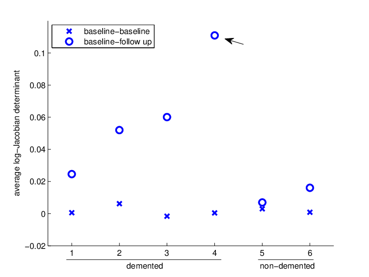
The use of first-order momenta allows us to interpret the result of the registrations and to relate the results to possible expansion of the ventricles. The volume change is indicated by the Jacobian determinant of the generated deformation at the deformation atoms as well as by the divergence of the first-order momenta. The latter is available directly from the registration parameters. We plot in Figure 7 the logarithm of the Jacobian determinant and the divergence for both the same day baseline-baseline registrations and for the baseline-follow up registrations. Patient are classified as demented, patient and as non-demented, and all patient have constant clinical dementia rating through the experiment. The time-span between baseline and follow up scan is 1.5-2 years with the exception of 3 years for patient four. As expected, the -Jacobian is close to zero for the same day baseline-baseline scans but it increases with the baseline-follow up registrations of the demented patients. In addition, the correlation between the -Jacobian and the divergence shows how the indicated volume change is related directly to the registration parameters; the parameters of the deformation atoms can in this way be directly interpreted as encoding the amount of atrophy.
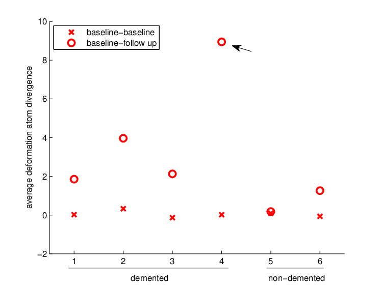
We chose two important parameters above: the kernel scale and the regularization term. The choice of one scale for all patients works well if the ventricles to be registered are of approximately the same size at the baseline scans. If the ventricles vary in size, the scale can be chosen individually for each patient. Alternatively, a multi-scale approach could do this automatically which suggests combining the method with e.g. the kernel bundle framework [27]. Depending on the image forces, the regularization term in (1) will affect the amount of expansion captured in the registration. Because of the low number of control points, we can in practice set the contribution of the regularization term to zero without experiencing non-diffeomorphic results. It will be interesting in the future to estimate the actual volume expansion directly using the parameters of the deformation atoms with this less biased model.
8 Conclusion and Outlook
We have introduced higher-order momenta in the LDDMM registration framework. The momenta allow compact representation of locally affine transformations by increasing the capacity of the deformation description. Coupled with similarity measures incorporating first-order information, the higher-order momenta improve the range of deformations reached by sparsely discretized LDDMM methods, and they allow direct capture of first-order information such as expansion and contraction. In addition, the constitute deformation atoms for which the generated deformation is directly interpretable.
We have shown how the partial derivative reproducing property implies singular momentum for the higher-order momenta, and we used this to derive the EPDiff evolution equations. By computing the forward and backward variational equations, we are able to transport gradient information and derive a matching algorithm. We provide examples showing typical deformation coded by first-order momenta and how images can be registered using a very few parameters, and we have applied the method to register human brains with progressing atrophy.
The experiments included here show only a first step in the application of higher-order momenta: the representation may be applied to register entire images; merging the method with multi-scale approaches will increase the description capacity and may lead to further reduction in the dimensionality of the representation. Combined with efficient implementations, higher-order momenta promise to provide a step forward in compact deformation description for image registration.
References
- [1] Vincent Arsigny, Olivier Commowick, Nicholas Ayache, and Xavier Pennec, A fast and Log-Euclidean polyaffine framework for locally linear registration, J. Math. Imaging Vis., 33 (2009), pp. 222–238.
- [2] Vincent Arsigny, Olivier Commowick, Xavier Pennec, and Nicholas Ayache, A Log-Euclidean framework for statistics on diffeomorphisms, in MICCAI 2006, 2006, pp. 924–931.
- [3] Vincent Arsigny, Xavier Pennec, and Nicholas Ayache, Polyrigid and polyaffine transformations: A novel geometrical tool to deal with non-rigid deformations – application to the registration of histological slices, Medical Image Analysis, 9 (2005), pp. 507–523.
- [4] M. Faisal Beg, Michael I. Miller, Alain Trouvé, and Laurent Younes, Computing large deformation metric mappings via geodesic flows of diffeomorphisms, IJCV, 61 (2005), pp. 139–157.
- [5] F. L. Bookstein, Linear methods for nonlinear maps: Procrustes fits, thin-plate splines, and the biometric analysis of shape variability, in Brain warping, Academic Press, 1999, pp. 157–181.
- [6] Yan Cao, M. I Miller, R. L Winslow, and L. Younes, Large deformation diffeomorphic metric mapping of vector fields, IEEE Transactions on Medical Imaging, 24 (2005), pp. 1216–1230.
- [7] GE Christensen, RD Rabbitt, and MI Miller, Deformable templates using large deformation kinematics, Image Processing, IEEE Transactions on, 5 (2002).
- [8] Colin J Cotter and Darryl D Holm, Singular solutions, momentum maps and computational anatomy, nlin/0605020, (2006).
- [9] Sune Darkner and Jon Sporring, Generalized partial volume: An inferior density estimator to parzen windows for normalized mutual information, in Information Processing in Medical Imaging, vol. 6801, Springer, 2011, pp. 436–447.
- [10] Paul Dupuis, Ulf Grenander, and Michael I Miller, Variational problems on flows of diffeomorphisms for image matching, (1998).
- [11] Stanley Durrleman, Marcel Prastawa, Guido Gerig, and Sarang Joshi, Optimal data-driven sparse parameterization of diffeomorphisms for population analysis, Proc. of the Information Processing in Medical Imaging Conference, IPMI, 22 (2011), pp. 123–134.
- [12] Gregory E. Fasshauer and Qi Ye, Reproducing kernels of generalized sobolev spaces via a green function approach with distributional operators, Numerische Mathematik, (2011).
- [13] N. C. Fox, E. K. Warrington, P. A. Freeborough, P. Hartikainen, A. M. Kennedy, J. M. Stevens, and M. N. Rossor, Presymptomatic hippocampal atrophy in alzheimer’s disease, Brain, 119 (1996), pp. 2001 –2007.
- [14] Laurent Garcin, Thechniques de Mise en Correspondance et Détection de Changements, PhD thesis, 2005.
- [15] Joan Glaunès, Transport par difféomorphismes de points, de mesures et de courants pour la comparaison de formes et l’anatomie numérique, PhD thesis, Université Paris 13, Villetaneuse, France, 2005.
- [16] Ulf Grenander, General Pattern Theory: A Mathematical Study of Regular Structures, Oxford University Press, USA, Feb. 1994.
- [17] Monica Hernandez, Matias Bossa, and Salvador Olmos, Registration of anatomical images using paths of diffeomorphisms parameterized with stationary vector field flows, International Journal of Computer Vision, 85 (2009), pp. 291–306.
- [18] William M. Wells III, Paul Viola, Hideki Atsumi, Shin Nakajima, and Ron Kikinis, Multi-Modal volume registration by maximization of mutual information, Medical Image Analysis, 1 (1996), pp. 35 – 51.
- [19] Clifford R. Jack, Ronald C. Petersen, Yue Cheng Xu, Stephen C. Waring, Peter C. O’Brien, Eric G. Tangalos, Glenn E. Smith, Robert J. Ivnik, and Emre Kokmen, Medial temporal atrophy on MRI in normal aging and very mild alzheimer’s disease, Neurology, 49 (1997), pp. 786 –794.
- [20] Daniel S Marcus, Anthony F Fotenos, John G Csernansky, John C Morris, and Randy L Buckner, Open access series of imaging studies: longitudinal MRI data in nondemented and demented older adults, Journal of Cognitive Neuroscience, 22 (2010), pp. 2677–2684. PMID: 19929323.
- [21] X. Pennec, R. Stefanescu, V. Arsigny, P. Fillard, and N. Ayache, Riemannian elasticity: A statistical regularization framework for non-linear registration, in MICCAI 2005, 2005, pp. 943–950.
- [22] J. P.W Pluim, J. B.A Maintz, and M. A Viergever, Image registration by maximization of combined mutual information and gradient information, IEEE Transactions on Medical Imaging, 19 (2000), pp. 809–814.
- [23] Alexis Roche, Grégoire Malandain, Xavier Pennec, and Nicholas Ayache, The correlation ratio as a new similarity measure for multimodal image registration, in Proceedings of the First International Conference on Medical Image Computing and Computer-Assisted Intervention, MICCAI ’98, Springer-Verlag, 1998, p. 1115–1124. ACM ID: 709612.
- [24] Alexis Roche, Xavier Pennec, Grégoire Malandain, and Nicholas Ayache, Rigid registration of 3D ultrasound with MR images: a new approach combining intensity and gradient information, IEEE Transactions on Medical Imaging, 20 (2001), pp. 1038—1049.
- [25] D Rueckert, L I Sonoda, C Hayes, D L Hill, M O Leach, and D J Hawkes, Nonrigid registration using free-form deformations: application to breast MR images, IEEE Transactions on Medical Imaging, 18 (1999), pp. 712–721. PMID: 10534053.
- [26] Christof Seiler, Xavier Pennec, and Mauricio Reyes, Geometry-Aware multiscale image registration via OBBTree-Based polyaffine Log-Demons, in Medical Image Computing and Computer-Assisted Intervention - MICCAI, Toronto, Canada, 2011.
- [27] Stefan Sommer, Mads Nielsen, Francois Lauze, and Xavier Pennec, A Multi-Scale kernel bundle for LDDMM: towards sparse deformation description across space and scales, in IPMI 2011, Springer, 2011.
- [28] Stefan Sommer, M. Nielsen, and X. Pennec, Sparse multi-scale diffeomorphic registration: the kernel bundle framework, To appear in Journal of Mathematical Imaging and Vision.
- [29] J.-P. Thirion, Image matching as a diffusion process: an analogy with maxwell’s demons, Medical Image Analysis, 2 (1998), pp. 243–260.
- [30] Alain Trouvé, An infinite dimensional group approach for physics based models in patterns recognition, 1995.
- [31] M. Vaillant, M.I. Miller, L. Younes, and A. Trouvé, Statistics on diffeomorphisms via tangent space representations, NeuroImage, 23 (2004), pp. S161–S169.
- [32] Tom Vercauteren, Xavier Pennec, Aymeric Perchant, and Nicholas Ayache, Diffeomorphic demons: efficient non-parametric image registration, NeuroImage, 45 (2009), pp. 61–72.
- [33] Younes, Constrained diffeomorphic shape evolution, submitted to foundations Comp Math, (2011).
- [34] Laurent Younes, Shapes and Diffeomorphisms, Springer, 2010.
- [35] Ding-Xuan Zhou, Derivative reproducing properties for kernel methods in learning theory, Journal of Computational and Applied Mathematics, 220 (2008), pp. 456–463.
- [36] Xiahai Zhuang, S. Arridge, D. J Hawkes, and S. Ourselin, A nonrigid registration framework using spatially encoded mutual information and Free-Form deformations, IEEE Transactions on Medical Imaging, 30 (2011), pp. 1819–1828.