Fast convolution based method for computing the signed distance function and its derivatives: Linear solution to the non-linear eikonal problem
Abstract
We present a fast convolution-based technique for computing an approximate, signed Euclidean distance function on a set of 2D and 3D grid locations. Instead of solving the non-linear, static Hamilton-Jacobi equation (), our solution stems from first solving for a scalar field in a linear differential equation and then deriving the solution for by taking the negative logarithm. In other words, when and are related by and satisfies a specific linear differential equation corresponding to the extremum of a variational problem, we obtain the approximate Euclidean distance function which converges to the true solution in the limit as . This is in sharp contrast to techniques like the fast marching and fast sweeping methods which directly solve the Hamilton-Jacobi equation by the Godunov upwind discretization scheme. Our linear formulation results in a closed-form solution to the approximate Euclidean distance function expressible as a discrete convolution, and hence efficiently computable using the fast Fourier transform (FFT). Our solution also circumvents the need for spatial discretization of the derivative operator. As , we show the convergence of our results to the true solution and also bound the error for a given value of . The differentiability of our solution allows us to compute—using a set of convolutions—the first and second derivatives of the approximate distance function. In order to determine the sign of the distance function (defined to be positive inside a closed region and negative outside), we compute the winding number in 2D and the topological degree in 3D, whose computations can also be performed via fast convolutions. We demonstrate the efficacy of our method through a set of experimental results.
Keywords:
distance transform; convolution; fast Fourier transform; winding number; topological degree; Green’s function2010 MSC
65D18, 65M801 Introduction
Euclidean distance functions (more popularly referred to as distance transforms) are widely used in image analysis and synthesis [1]. The task here is to assign at each grid point a value corresponding to the Euclidean distance to its nearest neighbor from a given point-set. Formally stated: given a point-set where is the dimensionality of the point-set and a set of equally spaced Cartesian grid points , the Euclidean distance function problem requires us to assign
| (1.1) |
where represents its Euclidean norm. In computational geometry, this is the Voronoi problem [2, 3] and the solution can be visualized as a set of cones with the centers being the point-set locations . The Euclidean distance function problem is a special case of the eikonal equation where the forcing function is identically equal to one and hence satisfies the differential equation
| (1.2) |
everywhere, barring the point-set locations and the Voronoi boundaries where is not differentiable. Here denotes the gradients of . This is a nonlinear differential equation and an example of a static Hamilton-Jacobi equation.
Since the advent of the fast marching method [4], the literature is replete with pioneering works which have successfully tackled this problem. Fast marching is an elegant technique which solves for in time at the given grid locations using the Godunov upwind discretization scheme. The stems from the overhead of administering a priority queue data structure. The ingenious work in [5] gives an implementation of the fast marching method with a cleverly chosen untidy priority queue data structure. Faster methods like the fast sweeping method [6] employs Gauss-Seidel iterations and finds the solution for in . Though it is computationally nicer and easier to implement than the fast marching method, the actual number of sweeps required for convergence depends on the problem at hand—heuristically sweeps are required in dimensions. Fast sweeping methods have also been extended to the more general static Hamilton-Jacobi equation [7] and also for the eikonal equation on non-regular grids [8, 9]. A Hamiltonian approach to solve the eikonal equation can be found in [10]. Methods based on geometric consideration of the reverse Huygens’s principle can be seen in [11]. In [2], the distance function is extracted by constructing the Voronoi diagram that is shown to be optimally linear in the number of data points. Other sweeping based methods for constructing the Euclidean distance function includes the work in [12].
In this article we provide a detailed description and extend our previous work on computing the signed Euclidean distance functions from point-sets [13, 14]. Since our approach uses the standard discrete Fourier transform (DFT) formulation, we compute the distance function only from a discrete set of source points positioned in a regular Cartesian grid. Moving away from the DFT setting (and as a result sacrificing the speed of computation), extension of this algorithm to curves can be found in [15]. As we motivate our method from a variational perspective—which we consider to be simultaneously novel and illuminating compared to our previous formulations—the proofs involved here are quite different. The intriguing aspect of our approach is that the nonlinear Hamilton-Jacobi equation (1.2) is obtained in the limit as of a linear differential equation. Let denote the approximate Euclidean distance function (with the nature of the approximation made clear below). When we express as the exponent of a scalar field , specifically , and if is the solution to a specific variational problem satisfying its corresponding linear Euler-Lagrange equation, we show that converges to the true Euclidean distance function and its gradient magnitude () also satisfies (1.2) as . Consequently, instead of solving the non-linear Hamilton-Jacobi equation we solve for the function (taking advantage of its linearity), and then compute an approximate distance function from its exponent for small values of . This computational procedure would be approximately equivalent to solving the original Hamilton-Jacobi equation. Our linear approach results in a closed-form solution which can be expressed as a discrete convolution and computed in time using a fast Fourier transform (FFT) [16] where is the number of grid points. The major advantage of our method is that the closed-form solution circumvents the need for spatial discretization of the derivative operator in (1.2), a problem that permeates the Hamilton-Jacobi solvers [4, 6]. This accounts for improved accuracy of our technique as demonstrated in Section 6. However, a minor caveat of our method is that the resultant Euclidean distance function is an approximation since it is obtained for a small but non-zero value of , but nevertheless converges to the true solution as .
The linear approach gives only an unsigned distance function. We complement this by independently finding the sign of the distance function in time on a regular grid in 2D and 3D. We achieve this by obtaining the winding number for each location in the 2D grid and its equivalent concept, the topological degree in 3D. We show that just as in the case of the unsigned Euclidean distance function, the winding number and the topological degree computations can be written in closed-form, expressed as discrete convolutions and efficiently computed using FFTs. We are not aware of any previous work that uses the winding number and topological degree approaches to compute signed distance functions. Furthermore, it is not easy to obtain the gradient of the signed distance function via the Hamilton-Jacobi solvers due to the lack of differentiability of their solution. Since our method results in a differentiable closed-form solution, we can leverage it to determine these gradient quantities. As before, the gradients can also be expressed in the form of discrete convolutions and computed using FFT’s. The gradients themselves converge to their true values as . To our knowledge fast computation of the derivatives of the distance function on a regular grid using discrete convolutions is new.
The paper is organized as follows. In Section 2 we derive the linear equation formalism for the Euclidean distance function problem and show convergence of our solution to the true solution as . We provide an approximate closed-form solution to compute the distance function and give an error bound between the computed and true distance functions for a given value of . Section 3 explains how the closed-form solution can be represented in the form of a discrete convolution and computed using fast Fourier transforms. In Sections 4 and 5 we compute the winding number (in 2D), the topological degree (in 3D) and the derivatives of the distance function by again expressing these quantities as discrete convolutions. In Section 6 we provide anecdotal evidence for the usefulness of our method by furnishing both experimental results and comparisons to standard techniques. We finally conclude in Section 7.
2 Linear differential equation approach for Euclidean distance functions
Recall that our objective is to compute the Euclidean distance function defined in (1.1), at a set of grid locations from the point-set . To this end, consider the following variational problem for a function namely,
| (2.1) |
where is a free parameter independent of and is the domain of integration. Here, —a function whose definition depends on —represents the initial scalar field concentrated around the source locations in the limit as . We define as
| (2.2) |
where is chosen such that it is square integrable with its support sequentially converging towards the point source as approaches zero and asymptotically behaves like the square-root of a function centered around . The square integrability (to one) constraint changes its functional form in accordance with the spatial dimension, as explicated in the subsequent sections.
The Euler-Lagrange equation corresponding to the extremum of computed over the scalar field is given by the linear equation
| (2.3) |
where stands for the Laplacian operator. We may be tempted to replace in (2.3) with a combination of delta functions each centered around and obtain an inhomogeneous screened Poisson partial differential equation. But as the delta functions are not square-integrable, they cannot be incorporated into the variational framework given in (2.1). Defining as in (2.2) forces it to behave like the square-root of a function as and hence is square-integrable for all values of .
Armed with the above set-up we realize that when we relate and satisfies (2.3) asymptotically converges to the true solution in the limit as as elucidated in Section 2.2. Furthermore, even the functions in namely () converge to their true values () and hence the gradient magnitude satisfies the Hamilton-Jacobi equation ( 1.2) as . We prove the convergence analysis for the gradient functions in Section 5.1. This relationship motivates us to solve for the linear equation in (2.3) instead of the non-linear eikonal equation and then compute the distance function via
| (2.4) |
2.1 Solution for the Euclidean distance function
We now derive the solution for (in 1D, 2D and 3D) which satisfies (2.3) and then for using the relation in (2.4). Since it is meaningful to assume that approaches infinity for points at infinity, we can use Dirichlet boundary conditions at the boundary of an unbounded domain. The validity of our variational formalism even for an unbounded domain can be seen from [17]. Note that the variational approach only provides a mechanism to obtain the linear differential equation for in (2.3)—which is the main focus of our paper. The functional in (2.1) provides orienting intuition for the origin of the differential equation—hence the lack of a fully formal treatment. Using a Green’s function approach [18], we can write expressions for the solution . The form of the solution for [18] in 1D, 2D and 3D is given by11 1 The representation of Green’s function involves two variables and and its value depends on the difference . For brevity we express as in this paper.
1D:
| (2.5) |
2D:
| (2.6) |
where is the modified Bessel function of the second kind,
3D:
| (2.7) |
The solution for can then be obtained via convolution as
| (2.8) |
can then be recovered from its exponent using the relation 2.4.
2.2 Proofs of convergence
Since we require to be square integrable to one and behave
like a square-root of the function centered at as , its definition varies with the spatial dimension and is
given by:
1D:
| (2.9) |
2D:
| (2.10) |
3D:
| (2.11) |
In 2D and in 3D the grid location and the point source are represented by and and and respectively. The proofs of convergence of —obtained from the exponent of —to the true solution given in (1.1) as are relegated to A.
2.3 Closed-form expression
A careful study of the proof in A where we show convergence of to the true solution encourages us to approximate the integral —obtained as a result of convolving the Green’s function with —with at small values of . Here is the spatial dimension. This approximation is cogent for the following reasons:
- 1.
- 2.
Second, our proof technique given in Section 2.2 attests to the fact that substituting the integral by either or still allows us to establish convergence to the true solution. Since
(2.12) our approximation is sound for small values of .
- 3.
Third, it provides us with a closed-form solution for as described below.
Hence we approximate the solution for the scalar field as
| (2.13) |
at small values of . Here equals . The value of depends on the spatial dimension as explained in Section 2.2.
Based on the nature of the expression for the Green’s function , it is worth highlighting the following very important point. The Green’s function in either 1D, 2D or 3D takes the form
| (2.14) |
for and being constants greater than zero. In the limiting case of , if we define
| (2.15) |
for some constant , then and furthermore, the convergence is uniform for away from zero. Therefore, provides a very good approximation for the actual unbounded domain Green’s function as . For a fixed value of and , the difference between the Green’s functions is which is relatively insignificant for small values of and for all . Moreover, using also avoids the singularity at the origin in the 2D and 3D cases. The above observation motivates us to compute the solution for by convolving with —instead of the actual Green’s function as in (2.13)—to get
| (2.16) |
The approximate Euclidean distance function computed based on the relation in (2.4) is then given by
| (2.17) |
Since and are constants independent of and converge to zero as , they can be ignored while solving for at small values of . Hence the scalar field can be further approximated as
| (2.18) |
and the approximate Euclidean distance function equals
| (2.19) |
We would like to underscore that the approximate solution for given in (2.18) possesses many desirable properties.
- 1.
Notice that as at the given point-set locations . Using the relation in (2.4) we get as satisfying the initial conditions.
- 2.
For small values of the quantity can be replaced by where —the true Euclidean distance function. Hence we get
(2.20) - 3.
can be efficiently computed using the fast Fourier transform as discussed in Section 3.
Hence for all practical, computational purposes we consider the expression given in (2.18) as the solution for . The bound derived below between and highlights the proximity between the computed and actual Euclidean distance functions.
2.4 Error bound between the obtained and true Euclidean distance function
Let denote the index of the source-point closest to , i.e, . If lies on the Voronoi boundary, we may choose any one of the multiple closest source-points and label it as . Multiplying and dividing the expression for in (2.18) by we have
| (2.21) |
Since , the term equals one independent of when or strictly decreases and converges to zero as when . In either case, strictly increases and converges to in the limit as .
Moreover, we also get the inequality
| (2.22) |
and along with (2.21) gives the bound
| (2.23) |
which is very tight as: (i) it scales only as the logarithm of the cardinality of the point-set () and (ii) can be made arbitrarily small by choosing a small but non-zero value of .
3 Efficient computation of the approximate unsigned Euclidean distance function
We now provide a fast convolution-based method to compute an approximate distance transform on a set of grid locations . The solution for given in (2.18) at the grid locations can be represented as the discrete convolution between the functions
| (3.1) |
computed at the grid locations, with the function which takes the value at the point-set locations and at other grid locations, i.e,
| (3.2) |
where,
| (3.3) |
We would like to press the following point home. The Kronecker delta function used in the definition of in (3.2) is not a replacement for the function used to define in (2.2). We define to be a sum of Kronecker delta functions so that the solution for given in (2.18) at the grid locations can be written in the form of a discrete convolution.
By the convolution theorem [16], a discrete convolution can be obtained as the inverse Fourier transform of the product of two individual transforms, which for two sequences can be computed in time [19]. One just needs to compute the discrete Fourier transform (DFT) of the sampled version of the functions and , compute their point-wise product and then compute the inverse discrete Fourier transform. Taking the logarithm of the inverse discrete Fourier transform and multiplying it by gives the approximate Euclidean distance function. The algorithm is spelled out in Table 1.
| 1. | Compute the function at the grid locations. |
|---|---|
| 2. | Define the function which takes the value at the point-set locations |
| and at other grid locations. | |
| 3. | Compute the FFT of and , namely and respectively. |
| 4. | Compute the function . |
| 5. | Compute the inverse FFT of to obtain . |
| 6. | Take the logarithm of and multiply it by to recover |
| the approximate Euclidean distance function. |
3.1 Computation of the approximate Euclidean distance function in higher dimensions
Our technique has a straightforward generalization to higher dimensions. Regardless of the spatial dimension, the approximate Euclidean distance function () can be computed by exactly following the steps delineated in Table 1. It is worth accentuating that computing the discrete Fourier transform using the FFT is always irrespective of the spatial dimension22 2 Even though the actual number of grid points () increases with dimension the solution is always in the number of grid points.. Hence, in all dimensions can be computed at the given grid points in . This speaks for the scalability of our technique which is generally not the case with other methods like KD-Trees [3].
3.2 Numerical issues
In principle we should be able to run our technique at a very small value of and obtain impressive results. However, for values of very close to zero, tapers off very quickly and hence for grid locations which are far away from the point-set the convolution performed via FFT using a double precision-based implementation tends to be erroneous. To this end, we turned to the GNU MPFR multiple-precision arithmetic library which provides arbitrary precision arithmetic with correct rounding [20]. MPFR is based on the GNU multiple-precision library (GMP) [21]. It enables us to run our technique at low values of . Advanpix [22] is another software that supports arbitrary precision.
3.3 Is the aforesaid issue a major pitfall?
It is natural for a reader to feel that our proposed method suffers from a fundamental impediment of requiring high precision machinery to serve its purpose. While the concern seems genuine, we would like to underscore that our technique can still be implemented in 64-bit precision (double data type) at a slightly higher value of . In the last 4 decades we have seen rapid growth from 8-bit microprocessors (for e.g 8008 microprocessor launched by Intel in 1972) to the current 64-bit computing paradigm based on registers, address buses or data buses of that size supporting 64-bit data types. Keeping abreast with the current trend, we should expect 128-bit or even 256-bit computing to become the household norm eliminating the need for the additional multiple-precision libraries to avail our technique.
In the fast marching and the fast sweeping methods the incurred error is lower bounded by the grid width as they involve spatial discretization of the derivative operator. Unless we resort to a more finer grid—in the process increasing the number of grid locations —the correctness of these methods cannot be ameliorated. Our method escapes this difficulty altogether as it doesn’t require discretization. For a given grid consisting of grid locations, the accuracy only depends on the value of allowed by the underlying computing architecture which—as we argued—can be progressively set to smaller value with furtherance in technology.
4 Fast computation of signed distance functions
The solution for the approximate Euclidean distance function in (2.19) is lacking in one respect: there is no information regarding the sign of the distance function. This is to be expected since the distance function was obtained only from a set of points and not a closed curve (in 2D) or surface (in 3D). We now describe a new method for computing the signed distance function in 2D using winding numbers and in 3D using the topological degree.
4.1 Computing winding numbers
Assume that we have a closed, parametric curve . We seek to determine if a grid location in the set is inside the closed curve. The winding number is the number of times the curve winds around the point (if at all) with counterclockwise turns counted as positive and clockwise turns as negative. If a point is inside the curve, the winding number is a non-zero integer. If the point is outside the curve, the winding number is zero. If we can efficiently compute the winding number for all points on a grid w.r.t. to a closed curve, then we would have the sign information (inside/outside) for all the points. We now describe a fast algorithm to achieve this goal.
The change in angle of the curve is given by . Since we need to determine whether the curve winds around each of the points , define . Then the winding number for the grid point is
| (4.1) |
In our case, we have a piecewise linear curve
defined by a sequence of points
. As we also assume that the curve is closed,
the “next” point after is . The integral
in (4.1) then becomes a discrete summation and we
get
| (4.2) |
, where the notation denotes that for and . We can simplify the notation in (4.2) (and obtain a measure of conceptual clarity as well) by defining the “tangent” vector as
| (4.3) |
with the symbol indicating either coordinate. Using the tangent vector , we rewrite (4.2) as
| (4.4) |
We observe that in (4.4) is a sum of two discrete convolutions. The first convolution is between two functions and . The second convolution is between two functions and . The Kronecker delta function is defined (3.3). The functions and are defined as
| (4.5) |
Here we have abused the notation and let () denote the ()-coordinate of the grid point . Armed with these relationships, we rewrite (4.4) to get
| (4.6) |
which can be computed in time using FFT-based convolution simultaneously for all the grid points .
It is apparent from the definitions given in (4.5) that the functions , and are not well-defined at the origin . The convolution of and with the functions and in (4.6) will lead to ill-defined values for at the source locations . The values remain unscathed at other grid locations as the convolution operation just centers the and functions around the source points. But, as the winding numbers are not even defined at the source locations (they are defined only with respect to them), the seemingly ominous aforementioned problem does not pose any serious threat. In actuality, the functions , and can take on any arbitrary value at leading to arbitrary values for at the source locations, which is meaningless and needs to be ignored. Hence without loss of generality we set .
4.2 Computing topological degree
The winding number concept for 2D admits a straight forward generalization to 3D and higher dimensions. The equivalent concept is the topological degree which is based on normalized flux computations. Assume that we have an oriented surface in 3D [23] which is represented as a set of triangles. The triangle has an outward pointing normal and this can easily be obtained once the surface is oriented. (We vectorize the edge of each triangle. Since triangles share edges, if the surface can be oriented, then there’s a consistent way of lending direction to each triangle edge. The triangle normal is merely the cross-product of the triangle vector edges.) We pick a convenient triangle center (the triangle incenter for instance) for each triangle and call it . The normalized flux (which is very closely related to the topological degree) [24] determines the ratio of the outward flux from a point treated as the origin. If is outside the enclosed surface, then the total outward flux is zero. If the point is inside, the outward normalized flux will be non-zero and positive.
The normalized flux for a point is
| (4.7) |
This can be written in the form of convolutions. To see this we write (4.7) in component form:
| (4.8) |
which can be simplified as
| (4.9) |
where and . The Kronecker delta function is defined (3.3). This can be computed in time using FFT-based convolution for all the grid points simultaneously.
For the sake of clarity we explicitly show the generalization of the winding number to the topological degree by rewriting some of the calculations involved in computing the winding number. Recall that for every point on the discretized curve, we defined its tangent vector in (4.3). The outward pointing normal , at the point ( will point outwards provided are taken in the anti-clockwise order), is given by . Using the normal vector , (4.4) can be rewritten as
| (4.10) |
The similarity between (4.10) and (4.7) is conspicuous. This lends extra validity to the fact that the topological degree is just a generalization of the winding number concept. It is important to bear in mind that the computation of the winding numbers and the topological degree does not require arbitrary precision package as no exponentially decaying functions are involved.
5 Fast computation of the derivatives of the distance function
Just as the approximate Euclidean distance function can be efficiently computed in , so can the derivatives. This is important because fast computation of the derivatives of on a regular grid can be very useful in curvature computations. Below, we detail how this can be achieved. We begin with the gradients and for illustration purposes, the derivations are performed in 2D:
| (5.1) |
A similar expression can be obtained for . These first derivatives can be rewritten as discrete convolutions:
| (5.2) |
where and are as defined in (4.5) and and are given in (3.1) and (3.2) respectively.
The second derivative formulas are somewhat involved. Rather than hammer out the algebra in a turgid manner, we merely present the final expressions—all discrete convolutions—for the three second derivatives in 2D:
| (5.3) | |||||
where is as defined in (4.5). Since we can efficiently compute the first and second derivatives of the approximate Euclidean distance function everywhere on a regular grid, we can also compute derived quantities such as curvature (Gaussian, mean and principal curvatures) for the two-dimensional surface computed at the grid locations . In Section 6 we visualize the derivatives for certain shape silhouettes.
5.1 Convergence analysis for the derivatives
We now show convergence of the derivatives () obtained via (5.1) to their true value as . Recall that the true distance function is not differentiable at the point-source locations and on the Voronoi boundaries which corresponds to grid locations which are equidistant from two or more point sources. Hence it is meaningful to establish convergence only for grid locations whose closest source-point can be uniquely determined.
For the purposes of illustration we show the analysis in 2D. Let be the unique closest source-point for a grid location , i.e, . Then the true derivatives at the location are given by
| (5.6) |
Multiplying and dividing the (5.1) by , we get
| (5.7) |
where . Since , it follows that . Since all the other terms in (5.7) are independent of we get . The convergence analysis for to follows along similar lines.
Furthermore, the gradient magnitude for any non-zero value of will be strictly less than its true value . To see this consider (5.1) and for the sake of convenience define , and . Since , after simple algebraic manipulations we get
| (5.8) |
Since , from the Cauchy-Schwarz inequality we have . It is then easy to see that . We also provide experimental evidence in the subsequent section to corroborate this fact. Nevertheless, the magnitude value converges to 1 as at all the grid locations (barring the point-sources and the Voronoi boundaries) as the gradients themselves converge to their true values.
6 Experiments
In this section we demonstrate the usefulness of our fast convolution approach to computing Euclidean distance functions on a bounded 2D and 3D grid. As we discussed before in Section 3.2 we go beyond the precision supported by the double floating-point numbers (64 bits) and resort to the GNU multiple-precision library (GMP) and MPFR arbitrary precision packages to improve the computational accuracy of our technique. For the following experiments we used precision bits.
6.1 2D Experiments
Example 1: We begin by discussing the effect of on our method and establish that as the accuracy our method empirically improves. To this end, we considered a 2D grid consisting of points between and at a grid width of . We ran experiments randomly choosing grid locations as data points (point-set), for different values of ranging from to in steps of . For each execution and at each value of we calculated the percentage error as
| (6.1) |
where and are respectively the actual distance and the absolute difference of the computed distance to the actual distance at the grid point. Figure 2 shows the mean percentage error at each value of . Note that the error varies almost linearly with in accordance with the maximum error bound of proved in Section 2.4. The maximum value of the error at each value of is summarized in Table 3. The error is less than % at demonstrating the algorithm’s ability to compute accurate Euclidean distance functions.

| Maximum error | |
|---|---|
| 0.00005 | 0.5728% |
| 0.0001 | 1.1482% |
| 0.00015 | 1.7461% |
| 0.0002 | 2.4046% |
| 0.00025 | 3.1550% |
| 0.0003 | 4.0146% |
| 0.00035 | 4.9959% |
| 0.0004 | 6.1033% |
| 0.00045 | 7.3380% |
| Shape | Fast convolution | Fast sweeping |
|---|---|---|
| Horse | 2.659% | 2.668% |
| Hand | 2.182% | 2.572% |
| Bird | 2.241% | 1.895% |
Example 2: We pitted our algorithm against
the fast sweeping method [6] on a grid consisting
of points between and at a
grid spacing of . We ran experiments, each time randomly
choosing grid points as data points. We set
for our approach and ran the fast sweeping for
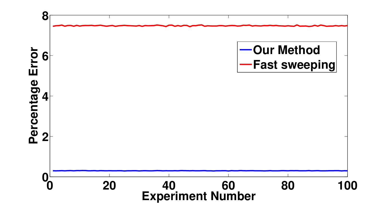
iterations more than enough for it to converge. The plot in Figure 2
shows the average percentage error calculated according to (6.1)
for both these techniques in comparison to the true Euclidean distance
function. From the plot it is clear that while the fast sweeping
method has a percentage error of around , our fast convolution method
method gave a percentage error of less than providing
much better accuracy.
Example 3: We then executed our algorithm
on a set of 2D shape silhouettes33
3
We thank Kaleem Siddiqi for
providing us with the set of 2D shape silhouettes
used in this paper.
. We sampled along the silhouette of these 2D shapes to generate the source points and then rounded the point cloud to the nearest grid points.
The grid size is and at
a grid width of . We set for our
method at . For the sake of comparison we
ran the fast sweeping method for iterations which was sufficient for it to converge.
The percentage errors calculated according to (6.1)
for both fast convolution and fast sweeping in comparison to the true Euclidean distance
function for these shapes are summarized
in Table 3. The true Euclidean distance function contour plots and those obtained
from fast convolution and fast sweeping are shown in Figure 3.


In order to differentiate between the grid locations that lie inside or outside to these shape silhouettes we computed the winding number for all the grid points simultaneously in using our convolution-based winding number method. Grid points with a winding number value greater than 0 after rounding were marked as interior points. In the the top part of Figure 4 we visualize the vector fields for all the interior points marked in blue (please zoom in to view the gradient vector fields). We see that our convolution-based technique for computing the winding number separates the interior grid points from the exterior with almost zero error. In the bottom part of Figure 4 we plot the distribution of the winding number values computed over all the interior and the exterior locations. Observe that for almost all the grid points, the winding number values are close to binary, i.e either 0 or 1, with a value of 0 marking the exterior points (as the curve doesn’t wind around them) and 1 representing interior locations.


In the top part of Figure 5 we plot the distribution of the gradient magnitude () values. Since we don’t solve for the true distance function and rather approximate it by (2.19) the magnitude of the gradients () obtained via (5.1) may not necessarily satisfy the Hamilton-Jacobi equation (1.2) for a non-zero value of and hence are not identically equal to 1. The reformulation of the derivatives given in (5.7) drives this point home. Nevertheless, we do observe that most of the gradient magnitude values (about ) are greater than 0.9. Also notice that all the gradient magnitudes are less than 1, as explained in Section 5.1.
In the bottom part of Figure 5 we visualize the gradient magnitude values as an image plot in tints of gray. Grid locations whose gradient magnitude values are in proximity to 1 are marked as white and the black color represent grid points whose gradient magnitude values are closer to its minimum value on the grid. From these image plots we see that the grid points which are either too close to the point-sources or those that lie along the medial axis (corresponding to the Voronoi boundaries for these shapes) incur maximum errors in their gradient magnitude values. As these grid locations are almost equidistant from multiple point-sources many of them contribute substantially to the summation value instead of just the nearest one leading to a relatively high induced error. From these visualizations we speculate that these inaccuracies when used prudently may actually aid in medial axis computation. We are currently investigating whether this can be achieved.


6.2 3D Experiments
Example 4: We also compared our Euclidean distance function fast convolution method with the fast sweeping method [6] and the exact Euclidean distance on the “Dragon” point-set obtained from the Stanford 3D Scanning Repository44 4 This dataset is available at http://graphics.stanford.edu/data/3Dscanrep/.. The common grid was , and and the grid spacing equals . The point cloud obtained from sampling the surface of the Dragon was rounded to the nearest grid points to generate the source locations. We ran our approach at and ran the fast sweeping method for 15 iterations which is sufficient for the Gauss-Seidel iterations to converge. We then calculated the percentage error for both these techniques according to (6.1). While the average percentage error for our approach when compared to the true distance function was just 1.306%, the average percentage error in the fast sweeping method was about 6.84%. Our FFT-based approach does not begin by discretizing the spatial differential operator as is the case with the fast marching and fast sweeping methods and this could help account for the increased accuracy. The iso-surface obtained by connecting the grid points at a distance of from the point-set determined by the true Euclidean distance function, fast convolution and fast sweeping are shown in Figure 6. The similarities between the plots provide anecdotal visual evidence for the usefulness of our approach.


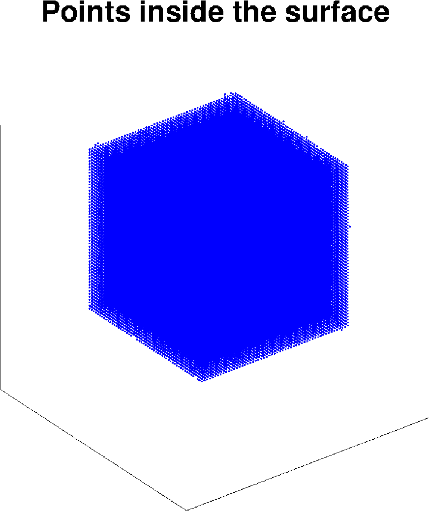
Example 5: We now demonstrate the efficacy of our fast convolution method for computing the topological degree. We considered a 3D grid, , and at a grid width of . Given a set of points sampled from the surface of a 3D object (and moved to the closest grid location), we triangulated the surface using built-in routines. We consider the incenter of each triangle to represent the data points . The normal for each triangle can be computed from the cross-product of the triangle vector edges. The direction of the normal vector was determined by taking the dot product between the position vector and the normal vector . For negative dot products, was negated to obtain a outward pointing normal vector. We then computed the topological degree for all the grid locations simultaneously in by running our fast convolution-based algorithm. Grid locations where the topological degree value equaled or exceeded were marked as inner points. Figure 7 shows the interior points for the three 3D objects—cube, sphere and cylinder (left to right).




7 Conclusion
In this work we began with a variational formalism for the Euclidean distance function problem. The variational problem with a free parameter balancing the data and gradient terms led to an Euler-Lagrange equation—a linear differential equation similar to a inhomogeneous, screened, Poisson equation. The intriguing aspect of our approach is that the non-linear Hamilton-Jacobi equation is embedded inside a linear differential equation and the solution is derived in the limiting case of . We obtained the solution for the function satisfying the Euler-Lagrange equation via a Green’s function approach and later approximated it with a closed-form solution which does not require spatial discretization of the derivative operator (unlike the Hamilton-Jacobi solvers) and is computed in at the grid locations using a FFT-based convolution method. The Euclidean distance is then recovered by taking the negative logarithm of . Since the scalar field is determined at a small but non-zero , the obtained Euclidean distance function is an approximation. We derived analytic bounds for the error of the approximation for a given value of and provided proofs of convergence to the true distance function as . The differentiability of our solution allowed us to express even the gradients of the distance function in closed-form, also written as convolutions. Finally, we demonstrated how our discrete convolution-based technique for computing the winding number in 2D and the topological degree in 3D aid in determining the sign of the distance function.
While Hamilton-Jacobi solvers have gone beyond the eikonal equation and regular grids—by providing efficient solutions even for the more general static Hamilton-Jacobi equation on irregular grids—in the current work we restrict ourselves only to computing the Euclidean distance function on regular grids. In the future we would like to follow the pioneering works of the fast marching and fast sweeping methods and try to extend our linear formalism to irregular grids and to the more general eikonal equation.
Appendix A Convergence analysis for the distance function
We provide the convergence of the distance function to its true value separately for each spatial dimension.
1D:
Using the expression for the 1D Green’s function we solve for as,
| (A.1) |
From the relation 2.4 we get
| (A.2) |
where and the integration region equals
| (A.3) |
For each define
| (A.4) |
Let denote the index of the source point closest to a given grid point , i.e, . Then for sufficiently small we have
| (A.5) | |||||
as for .
On the other hand, notice that for each , . Hence for small values of we also arrive at the inequality
| (A.6) | |||||
In order to see why the second step in the above relation holds, consider the two scenarios: (i) is not a point on the Voronoi boundary, and (ii) lies on the Voronoi boundary. If doesn’t lie on the Voronoi boundary, then exists a neighborhood around such that , . Since for sufficiently small values of , the aforementioned relation is true. On the flip side, if is a point on the Voronoi boundary, the closest source point is not uniquely defined. However we can unambiguously choose a closest source point and a such that for , . These observations buttress the above inequality.
Since , and approach zero as , we obtained the desired result namely, .
2D:
Based on the expression for the 2D Green’s function and the relation 2.4, we get
| (A.7) |
where and the integral region equals
| (A.8) |
Defining
| (A.9) |
for each and closely following the arguments illustrated for the 1D case, we have
| (A.10) |
for small values of , where . As considered above, denotes the index of the source point () closest to . Similar to the 1D case, note that for where is the closest source-point to . Using the relation when we also get
| (A.11) |
as . If we let , then similar to the 1D case we arrive at the inequality,
| (A.12) | |||||
As when , it follows that
| (A.13) |
for small values of . Since approach as
and the rest of the terms tend to zero, we obtain the
desired result namely,
.
3D:
By exactly following the line of argument delineated for the 1D and the 2D
case where we bound above and below by functions which
converge to the true Euclidean distance function as , we can prove that .
References
- [1] S. J. Osher, R. P. Fedkiw, Level set methods and dynamic implicit surfaces, Springer-Verlag, New York, NY, 2003.
- [2] A. Aggarwal, L. Guibas, J. Saxe, P. Shor, A linear time algorithm for computing the voronoi diagram of a convex polygon, in: STOC, ACM, 1987, pp. 39–45.
- [3] M. D. Berg, O. Cheong, M. V. Kreveld, M. Overmars, Computational geometry: Algorithms and applications, Springer-Verlag, New York, NY, 2008.
- [4] J. A. Sethian, A fast marching level set method for monotonically advancing fronts, Proc. Nat. Acad. Sci. 93 (4) (1996) 1591–1595.
- [5] L. Yatziv, A. Bartesaghi, G. Sapiro, O(N) implementation of the fast marching algorithm, J. Comp. Phys. 212 (2) (2006) 393–399.
- [6] H. K. Zhao, A fast sweeping method for eikonal equations, Math. Comp. 74 (250) (2005) 603–627.
- [7] C. Y. Kao, S. J. Osher, Y. H. Tsai, Fast sweeping methods for static Hamilton-Jacobi equations, SIAM J. Num. Anal. 42 (6) (2004) 2612–2632.
- [8] J. Qian, Y. T. Zhang, H. K. Zhao, Fast sweeping methods for eikonal equations on triangular meshes, SIAM J. Num. Anal. 45 (1) (2007) 83–107.
- [9] C. Y. Kao, S. J. Osher, J. Qian, Legendre-transform-based fast sweeping methods for static Hamilton-Jacobi equations on triangulated meshes, J. Comp. Phys. 227 (24) (2008) 10209–10225.
- [10] K. Siddiqi, A. Tannenbaum, S. Zucker, A Hamiltonian approach to the eikonal equation, in: EMMCVPR, Vol. 1654 of LNCS, Springer, 1999, pp. 1–13.
- [11] Y. H. R. Tsai, Rapid and accurate computation of the distance function using grids, J. Comp. Phys. 178 (2002) 175–195.
- [12] P. E. Danielsson, Euclidean distance mapping, Comp. Graph. Image Proc. 14 (3) (1980) 227–248.
- [13] K. S. Gurumoorthy, A. Rangarajan, A Schrödinger equation for the fast computation of approximate Euclidean distance functions, in: SSVM, Vol. 5567 of LNCS, Springer, 2009, pp. 100–111.
- [14] A. Rangarajan, K. S. Gurumoorthy, A Schrödinger wave equation approach to the eikonal equation: Application to image analysis, in: EMMCVPR, Vol. 5681 of LNCS, Springer, 2009, pp. 140–153.
- [15] M. Sethi, A. Rangarajan, K. S. Gurumoorthy, The Schrödinger Distance Transform (SDT) for point-sets and curves, in: CVPR, IEEE Computer Society, 2012, pp. 198–205.
- [16] R. N. Bracewell, The Fourier transform and its applications, 3rd Edition, McGraw-Hill, New York, NY, 1999.
- [17] G. Wahba, Spline models for observational data, Vol. 59 of CBMS-NSF Regional Conference Series in Applied Mathematics, SIAM, Philadelphia, PA, 1990.
- [18] M. Abramowitz, I. A. Stegun, Handbook of mathematical functions with formulas, graphs and mathematical tables, Dover, New York, NY, 1964.
- [19] J. W. Cooley, J. W. Tukey, An algorithm for the machine calculation of complex Fourier series, Math. Comp. 19 (90) (1965) 297–301.
- [20] L. Fousse, G. Hanrot, V. Lefévre, P. Pélissier, P. Zimmermann, MPFR: A multiple-precision binary floating-point library with correct rounding, ACM Trans. Math. Softw. 33 (2007) 1–15.
- [21] G. Torbjörn, et al., GNU multiple precision arithmetic library 5.0.1 (June 2010).
- [22] Multiprecision computing toolbox for MATLAB (Advanpix LLC.) (2014).
- [23] A. Gray, Modern differential geometry of curves and surfaces with mathematica, 2nd Edition, CRC Press, Boca Raton, FL, 1997.
- [24] O. Aberth, Precise numerical methods using C++, Academic Press, San Diego, CA, 1998.