KCL-MTH-11-23
ITP-Budapest report No. 654
Excited state g-functions from the Truncated
Conformal Space
G. Takács 11
1
Email: takace@elte.hu and G.M.T. Watts 22
2
Email: gerard.watts@kcl.ac.uk
HAS Theoretical Physics Research Group,
1117 Budapest, Pázmány Péter sétány 1/A, Hungary
22footnotemark: 2Department of Mathematics, King’s College London,
Strand, London WC2R 2LS – UK
Abstract
In this paper we consider excited state g–functions, that is, overlaps between boundary states and excited states in boundary conformal field theory. We find a new method to calculate these overlaps numerically using a variation of the truncated conformal space approach. We apply this method to the Lee-Yang model for which the unique boundary perturbation is integrable and for which the TBA system describing the boundary overlaps is known. Using the truncated conformal space approach we obtain numerical results for the ground state and the first three excited states which are in excellent agreement with the TBA results. As a special case we can calculate the standard g-function which is the overlap with the ground state and find that our new method is considerably more accurate than the original method employed by Dorey et al.
1 Introduction
If a conformal field theory is defined on a domain with a boundary then boundary conditions need to be defined. In the simplest case of the unit disk, the boundary conditions are implemented through a boundary state. Such boundary states are not normalisable, but are uniquely determined by their overlaps with the normalisable, finite-energy states of the bulk system. The exact forms of the boundary states of all the conformal boundary conditions for many conformal field theories, and hence all these overlaps, have been known for some long time,
In this paper we consider non-conformal boundary conditions generated by a perturbation of a conformal boundary condition by the integral of a local field along the boundary. The resulting perturbed boundary condition can also be described by a boundary state which is uniquely specified by its overlaps with the bulk states. If the perturbation is integrable then it may be possible to calculate the overlaps using the Thermodynamic Bethe Ansatz (TBA). For such systems there is a distinguished basis of states and for each state there is an integral equation for the overlap. If the perturbation is not integrable then one needs an alternative method to calculate the overlaps and determine the boundary state.
One important numerical method to study perturbed conformal field theory is the Truncated Conformal Space Approach (TCSA). This was initiated by Yurov and Zamolodchikov [1] and used to study the finite-size spectrum of bulk perturbations of conformal field theories. It was adapted by Dorey et al to study the finite-size spectrum of boundary-perturbed conformal field theory [2], and it was shown by Dorey et al in [3] how this could be used to calculate the g–function, or ground state overlap with the boundary state. It was not possible, however, to use this method or a modification to calculate overlaps of the boundary state with excited bulk states.
Here, we present an alternative method based on the TCSA inspired by the work of Zamolodchikov on the partition function of a perturbed conformal field theory on a sphere [4] where the partition function on a sphere was calculated using the Schrödinger equation for a truncated system. The sphere was conformally mapped into the complex plane and the resulting system was formally the same as the usual truncated conformal space approach with a space-dependent coupling.
We calculate the boundary state overlaps as one point functions of bulk fields on a disk. The disk can be conformally mapped to the upper half plane and the one-point function of a bulk field is mapped to the expectation value of the bulk field in a state corresponding to a half-disk with a time-dependent coupling to a boundary field. We then truncate the Hilbert space and numerically integrate the perturbation to find the state for the half-disk. Once the half-disk state has been found, it is only necessary to calculate the matrix elements of the required bulk field to find the overlap of the bulk state with the boundary state.
There are some technical difficulties applying this method to higher excited states arising from the form of the TCSA expression for the bulk field expectation value which is similar to a Fourier expansion in the argument of the insertion point. Excited states correspond to repeated derivatives of the field and the derivatives of the Fourier series do not themselves converge. this can be handled by forcing convergence of the Fourier series (at the loss of some information) which gives numerically satisfactory results at the expense of some complication in the calculational scheme.
We apply this method to the simplest perturbed boundary conformal field theory, the Lee-Yang model, which was the model studied in [2, 3] and has the advantage that the overlaps can also be calculated using the TBA method and we find excellent agreement.
The layout of the paper is as follows. In section 2 we outline the general truncated space method and in section 3 we apply it to the ground state and first excited state in the Lee-Yang model. In section 4 we consider the next two excited states and explain how to force convergence of method. We outline the TBA method used in an appendix.
2 -functions and perturbed conformal field theory
Our aim is to calculate the overlap of a bulk state with the boundary state corresponding to a perturbation of a conformal boundary condition on the boundary of the disc by the insertion of on this boundary. We take to be a primary boundary field of conformal dimension . We shall denote such an overlap by where labels the particular bulk state. The most natural way to calculate this one point function is to expand the exponential and consider it as a perturbative expansion with repeated insertions of the boundary field. If , then such a function will have a regular expansion in powers of for small (where is the mass dimension of the coupling constant ), but for large the dominant term is non-perturbative:
| (2.1) |
where is the boundary free energy per unit length and is the length of the boundary. While this is the natural consequence of a perturbative expansion, it is many ways more natural to consider the state perturbed boundary to interpolate between two conformal boundary conditions which requires subtracting the free energy term; this gives the definition of the (non-perturbative) -function as
| (2.2) |
We shall define the perturbed boundary state by the conformal normalisation so that the overlap gives with the bulk state the perturbative -function,
| (2.3) |
The overlap can be realised as the insertion of the field in the disk with boundary condition , where and it is this definition which is the basis of the TCSA method described below.
2.1 The TCSA approach to the disk
In order to use the TCSA method, we need to find a way in which the boundary field can be constructed as an operator acting on a Hilbert space (which can be truncated), or equivalently in which the system has a Hamiltonian description where the boundary field enters the Hamiltonian. We first outline the operator realisation and then the Hamiltonian description.
To have an operator action, once must choose “equal-time” surfaces to which one can associate a Hilbert space of states on these surfaces. For the boundary field to act, these surfaces must have boundaries, and the most natural surface is a line segment corresponding to equal time slices across an infinite strip. This is conformally equivalent to the upper half plane with the equal-time surfaces being semi-circles of constant radius, known as radial quantisation. We can map the interior of the unit disk (with coordinate ) to the upper half plane (with coordinate ) using the map
| (2.4) |
This map is shown in figure 1
The one-point function in the perturbed boundary condition becomes the matrix element of a field between states representing the interior of the unit semi-circle (with perturbed boundary condition) and the exterior (with perturbed boundary condition). Using the transformation property of primary spinless boundary fields,
| (2.5) |
we can write the state corresponding to the interior of the semi-circle of radius as
| (2.6) |
where and denotes radial ordering. The overlap is then
| (2.7) |
where (const.) is a constant normalisation factor and where is the image of the field under the map ; if is a spinless quasi-primary field of total conformal weight , this is the simple rescaling
| (2.8) |
otherwise it is more complicated.
The state satisfies the differential equation
| (2.9) |
and we can use (2.9) as the basis for a TCSA calculation. We can truncate the Hilbert space of the system at excitation level and solve the first order matrix differential equation for using the finite matrix truncations of . We can then take the matrix elements of in the truncated state and this is the TCSA approximation to the overlap.
2.2 Realisation as a Hamiltonian system
The calculation of the previous section can be recast in terms of a perturbed Hamiltonian (in the spirit of [4]) as follows. It is easiest to see the relation by mapping the disk to an infinite strip, by the further map
| (2.10) |
which maps the original disk to the strip (see figure 1. If then the lines can be taken as equal time slices and the Hamiltonian propagates in along the strip. The equation (2.9) is transformed into the Schrödinger equation in the interaction picture,
| (2.11) |
where is the -dependent Hamiltonian
| (2.12) |
This problem can be also be formulated in the Schrödinger picture in which case the relevant Hamiltonian is
| (2.13) |
It is this formulation which is directly comparable to the Hamiltonian formulation of the bulk model on the sphere in [4]. In practice we have used (2.9) to perform our TCSA calculations as it is numerically more stable.
We now turn to the calculation of the ground state and first excited state overlaps in the Lee-Yang model.
3 The Lee-Yang model
The Lee-Yang model has been used extensively as a test of exact and numerical methods because it is in many ways the simplest, and the convergence of the TCSA calculation of its spectrum is amongst fastest of all known models. In this context it is the simplest because it has only two conformal boundary conditions and a single integrable perturbation which connects them. It also has the fewest states at any particular excitation level so that the size of any TCSA truncation will be smallest in the Lee-Yang model. The details of the conformal and integrable descriptions of the boundary conditions can be found in [2, 3] and we only recall the most important details here.
We start with the description of the theory in the bulk. The Lee-Yang model is the minimal conformal field theory with . It is non-unitary and there are two highest weight representations of the Virasoro algebra which are relevant, with conformal weights and . If we denote these two highest weight representations by and then the Hilbert space of the bulk theory is
| (3.1) |
We take the bulk highest weight states to be and of conformal weight and respectively. The invariant state is but the ground state in the bulk theory is . It is convenient to normalise these states as
| (3.2) |
The state is associated to the primary field and satisfies
| (3.3) |
The Lee-Yang model has two conformal boundary conditions. We will adopt the conventions of [2] in which these are called and and the states associated to them on the unit disk are
| (3.4) |
where is the -value of the boundary condition , is the value of the disk partition function with boundary condition and are the usual Ishibashi states [5].
As described in [2], there is a single integrable flow between the boundary conditions and , the perturbed boundary conditions being denoted by where is the coupling to the unique relevant boundary field on the condition . This field has conformal weight and is denoted by .
The particular boundary conditions we are considering, both perturbed and unperturbed, are rotationally invariant and so the only states which have non-zero overlap must have zero spin, that is they must have equal and eigenvalues. The lowest lying zero-spin states, their conformal weights and the fields to which they correspond are in table 1. We’ll denote the overlap with the -th excited state as and the associated -function as . It is a property of the conformal boundary states that the overlap with a normalised bulk state only depends on the representation in which it lies, so that in particular we have
| (3.5) |
We also need the description of the boundary condition in the upper-half plane operator picture. In this formulation, the unperturbed Hilbert space is that of a strip with the boundary condition on both sides and is the direct sum of the two Virasoro algebra representations in the Lee-Yang model,
| (3.6) |
We denote the highest weight states in the UHP picture as and respectively. The ground state is which corresponds to the insertion of the boundary field at the origin of the model on the upper half plane. We again choose to normalise these states as
| (3.7) |
The expectation value of any operator on the disk with the conformal boundary condition is now given by
| (3.8) |
where is the map (2.4) from the disk to the UHP. In particular we recover the partition function for the identity operator ,
| (3.9) |
For the ground state entropy we use the operator and . With the result we get
| (3.10) |
We now turn to the overlaps with the excited boundary states.
The first overlap studied was the ground state overlap, the original -function of [6] for which a TBA formulation was first described in [7]. Subsequently, it was shown in [8] that the -function was the first of an infinite set of excited state -functions which arose as the eigenvalues of generalised transfer matrices satisfying a so-called -system. This -system has been put into an orthodox conformal field theory context by Runkel [9]. In the case of the Lee-Yang model the -system is identical to the so-called -system and Bazhanov et al also showed how to find the TBA system for excited state -functions and solved it for the first excited state. The ground state -function was compared to an alternative TCSA calculation of in [3] with reasonable agreement. Here we state the expected relation between the and functions:
| (3.11) |
where , and we have suppressed the -dependence of the state . The -functions depend on a rapidity which is related to by [8]
| (3.12) |
The extra factor of between the formula here and that in [3] arises because the boundary of the unit disk has length and it is the combination which is relevant to this equation.
We now describe the TCSA approximation and in particular the lowest level truncation where the UHP Hilbert space is restricted to just two states.
3.1 TCSA method and results
We have used the TCSA approximation to the differential equation (2.11) to calculate approximations to the state and then calculated the exact expectation value of the fields and in these approximate states for truncation levels 0 up to 20, that is for systems of size 2 up to 323. To illustrate the method, we consider here the case of truncation to level 0, that is we truncate the Hilbert space to just the two highest weight states and , and construct the TCSA equations for the upper half plane state (2.9) explicitly.
We take the state to be truncated to just the highest weight states and , so that it is determined by just two functions and ,
| (3.13) |
The actions of the field on these states are (for both positive and negative)
| (3.14) | |||||
| (3.15) | |||||
This means that truncating (2.9) to the two states gives the differential equation
| (3.16) |
which should be solved subject to the initial conditions
| (3.17) |
The result is the TCSA estimate
| (3.18) |
From this we can calculate the TCSA estimates of the two -functions,
| (3.19) | |||||
| (3.20) |
To complete the calculation of the -functions, we need the one-point functions of the field on the UHP, which are in appendix A and the re-scalings from (3.11), resulting in
| (3.21) | |||||
| (3.22) |
We used Mathematica [20] built-in routines to solve the matrix differential equations with satisfactory results. Already the accuracy obtained using just a truncation to 2 states is quite surprising. We list some numerical results in table 2 and in figure 2 we plot the 2-state truncation estimates for the functions and together with the exact results calculated using the TBA equations of [8] and the results of second and third order perturbation theory (see appendix B).
Although the agreement with the functions and as plotted in figure 1. of [8] is impressive, this is in main due to the dominance of the functions by the boundary free energy term which means that the functions grow rapidly and are hard to show on this particular plot. To remove this factor, we instead plot the the -functions and which interpolate the UV and IR values of and respectively, using [3]
| (3.23) |
In figure 3 we show tha TCSA estimates (for truncation levels 0 and 20) and TBA values of and , along with the result of a Padé approximant extrapolation in truncation level to .
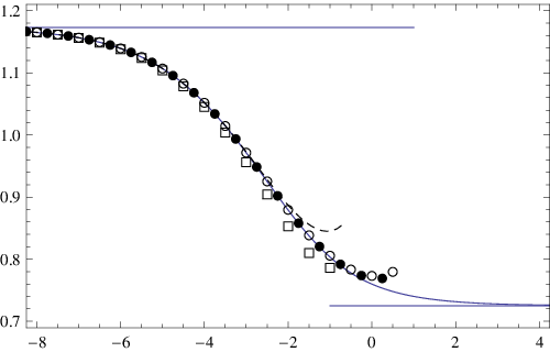


As can be seen in figure 3(a), the estimate of and from the level zero truncation is already quite good and convergence improves rapidly with increasing truncation level, so that for level 20 it is qualitatively accurate up to . The main error seems to come from errors in the extensive boundary energy per unit length which can be attributed to an effective coupling constant renormalisation in the TCSA method [10]. Rather than attempt to incorporate these effects in the differential equation, we can remove the error from the boundary free energy by looking at the ratio of the -functions, which is plotted in figure 4.
We can attempt to improve the accuracy of our estimates by using an extrapolation method to estimate the limit of the TCSA data. We have used two ways of approaching the (described in section 4) limit and three different extrapolation methods. In all cases, all three extrapolation methods gave the similar results, with Wynn’s method [11] based on Padé approximants being the best. The two different ways of approaching the limit, while very similar for and , differed considerably for some higher excited states. The simplest method, considering the level approximation to be given by the full TCSA expression (2.7), failed to be effective for fields of weight greater than 2, and we had to use a second approximation to get an effective extrapolation to . We illustrate this in table 3 with the TCSA estimates of and at for together with the two Padé extrapolations labelled and and the TBA value. We also include the values of , , and which will be discussed in the next section, together with a discussion of the two extrapolations.
To conclude this section, we discuss the comparison with the previous TCSA estimation of in [3]. In that paper, was estimated from the scaling with the strip width of the cylinder partition function calculated as a trace over the space of states on the strip. This was a rather convoluted calculation which nevertheless showed good agreement with the exact functions. In figure 3(a) we include the old TCSA estimate from the level 18 truncation (using the exact boundary free energy per unit length as shown in [3]); as can be seen, the new method is much better. The old TCSA estimate could be improved by fitting the boundary free energy term to account for the renormalisation of the coupling constant, as can the new TCSA estimate by extrapolation in , and the new method again gives better results.
4 Higher excited states in the Lee-Yang model
We can continue to apply the same method to the higher excited states in the Lee-Yang model. The next four states are given in table 1 and three of the corresponding fields are given by simple derivatives of the primary field . We can calculate these by directly taking the derivative of the one-point function on the perturbed disc of , which we discuss in appendix C. The fourth excited state corresponds to the field and we discuss its matrix elements in appendix D. The results for the excited state functions to at in table 3. As can be seen, these are convergent for the first three states but oscillatory and divergent for to . The behaviour of these divergent cases is of an increasing oscillating series, typical of a divergent perturbation expansion.
This immediately suggests that one might be able to re-sum the divergent series and obtain useful results. We have tried Euler, Cesaro and Padé extrapolation (using Wynn’s method [11]) and these all gave similar results. They all improve the results ofr to , are all able to produce a result correct to a few percent for the divergent series and but all fail on . As a consequence we considered different ways to approach limit, that is we constructed a different TCSA approximation at each level which would agree for convergent series, but could give better results for divergent series. Looking at the matrix elements of the fields it seemed that these were organised by the total excitation level of the states and rather than the maximum level. We consequently defined two series as follows. We first denote the contributions at excitation level to the level TCSA approximation to the state by , so that
| (4.1) |
For any operator , we then define two series of polynomials
| (4.2) |
The direct TCSA approximation at level is given by . If the TCSA approximation converges in then both and converge to the same answer; if the TCSA expression diverges then the two polynomials can differ considerably and we can take the Padé approximants to and at and see if they provide useful estimates of the answer. As an example, we consider and the truncation to level 12 at . The polynomials are
| (4.3) |
We see that neither of these is close to the exact result of -113.6. Instead we take the Padé approximants
and find the Padé approximant estimates and the exact (TBA) answer are
| (4.4) |
We see that the -approximation is reliable and the -approximation is not. This is repeated for the other divergent cases of and - the -estimate is always better than the -estimate. It is worth noting that for the convergent cases there is very little difference between the two, but that the -estimate is very slightly better than the -estimate since the -polynomial includes more (convergent) matrix elements than the -polynomial.
We show the resulting plots for the ratios of the -extrapolated TCSA results at level 20 in figure 5. We see that the ratios, which are the physical content of the -functions, are all well described by the -extrapolated TCSA data up to approximately the same value of , which is the value at which the TCSA Hamiltonian on a strip also fails to give an accurate description for the 5th excited state of the spectrum.
5 Conclusions
We have found a new and effective way to calculate the overlaps of perturbed boundary states with bulk states giving excited state -functions, or equivalently -functions. We have studied these in some detail in the Lee-Yang model (in which the -functions are identically equal to the -functions) and shown that the estimates are good for the whole range of values for which the TCSA method on the strip is applicable. Even using a truncation to just two states, the results are better than second order perturbation theory. It is disappointing, although perhaps not surprising, that the TCSA estimates computed directly are divergent for the states of conformal weight greater than 2, but we have found an efficient extrapolation method which works effectively for all the states we have considered.
This new TCSA method can be applied to any boundary perturbation for which the boundary couplings are known and is not restricted to integrable models, as was the case here. The method also has immediate scope for generalisation to include massive, or bulk, perturbations, which should help check any conjectured TBA equations for the bulk excited state -functions which are complicated by the extra infinite series required to account for the bulk corrections [16, 17]. It can also be applied to study defect matrix elements (which are boundary state overlaps in the double model through the usual mirror trick) and calculate the reflection and transmission coefficients defined in [18] and help clarify the nature of the endpoints of the defect flows studied in [19].
Acknowledgements
GMTW would like to thank ELTE for hospitality at the start of this project and STFC grant ST/G000395/1 for support and Zoltán Bajnok, Patrick Dorey, Roberto Tateo and Ingo Runkel for useful discussions. GT was partially supported by the Hungarian OTKA grant K75172. The TCSA calculations were performed using Mathematica [20].
Appendix A The Lee-Yang conformal data
The coefficients appearing in the boundary states (3.4) are
| (A.5) | |||
| (A.6) |
The various structure constants used in this paper are
where
| (A.10) |
Finally, the one-point functions of on the UHP are given in terms of and as
| (A.11) |
where and .
Appendix B Perturbation theory
It is straightforward to obtain one or two orders of the perturbation epansions of the functions . For the -function this was given in [8] and the conformal theory perturbation discussed in [3]. Here we write them in terms of rather than :
| (B.12) |
The function , the disk partition function, can be expanded out to third order as
| (B.13) |
Similarly, and can be expanded to second order and to third order based on conformal perturbation theory; beyond these orders the integrals become difficult to evaluate exactly, although use of the Y-function relation (E.32) does allow one to calculate one further order for and three further orders for as the coefficients in the perturbation expansion are severely constrained by this relation [8], and so obtain
| (B.14) | |||||
| (B.15) | |||||
where . These are also shown in figure 2
It is rather harder to calculate the -dependent function as the integrals again become harder. To first order we have (for a disk of radius 1)
| (B.16) |
Appendix C expectation values
Of the first four excited states given in table (1), three are derivatives of the primary field . We can calculate the overlaps with these states by directly taking the derivative of the one-point function of . Here we show how this is defined in our TCSA approach. We use the coordinates on the unit disk and on the UHP, related by (2.4). In these coordinates
| (C.17) |
The general form of the expectation value of an operator on the disk is given by (3.8) and the transformation property of the primary field is given by (2.5), so that
| (C.18) | |||||
We then used
| (C.19) |
to arrive at
| (C.20) |
The matrix elements of can be calculated in the usual way from the highest weight matrix elements (A.11). Given these, the TCSA estimate takes the form
| (C.21) |
where
| (C.22) |
and the coefficient functions have the form
| (C.23) |
For the level 0, two-state truncation with , these functions are
| (C.24) |
The map is conformal and the Laplacian in these coordinates is
| (C.25) |
While the functions converge in , the repeated action of leads to a failure of convergence, which in this case is happens first for with two applications of .
Appendix D expectation values
The field is quasi-primary and transforms under the Mobius map (2.4) as
| (D.26) |
which gives the expectation value on the perturbed disk as
| (D.27) | |||||
The product is regular and its matrix elements can be worked out in the truncated conformal space using the normal ordering relation identity appropriate for the TCSA method,
| (D.28) | |||||
where and . This choice of ordering means that the matrix elements of in the truncated space can be calculated exactly using the expansion of the right-hand-side of (D.28) in the truncated conformal space. To work out the level zero TCSA approximation, we just need the expectation value in a highest weight state,
| (D.29) | |||||
Putting this all together, we find the level zero TCSA approximation to the disk one-point function of the normalised field is
| (D.30) |
As is immediately obvious, this does not have the expected rotationally-invariant form , since the TCSA method breaks rotational invariance.
Appendix E TBA equations in the Lee-Yang model
The scaling Lee-Yang model is the perturbation of the conformal minimal model by the relevant field :
It has a single particle of mass in the spectrum with the two-particle matrix
The ground state TBA of the SLYM has the form [12]
where
The excited state levels can be determined by solving the equations [13, 8]
| (E.31) | |||||
where is the number of particles present in the state with the singularity positions corresponding to their rapidities. For large volumes, the integral terms can be dropped and a straightforward calculation shows that the singularity positions have the form
where the particle rapidities solve the Bethe-Yang equations
with (for odd) or (for even) labelling the particular state in question.
The function of the given level can be defined as
and it satisfies the functional relations [14]
| (E.32) |
These equations can be solved by iteration: the Bethe-Yang equations give a starting point for the position of the singularities, which can then be used to iterate the system (E.31). For a given position of singularities the function can be updated by iterating the integral equations, and then the positions of the singularities can be refined by solving the equations
for the real variables given by the real and imaginary parts of . This can be accomplished by the multidimensional Newton method; the derivative matrix of the equations with respect to the variables can be expressed by taking the derivative of the integral equation in (E.31).
To describe the states in the minimal model, we consider the so-called kink limit of the above TBA system describes a chiral (right moving) version of the Lee-Yang minimal model. The variable must be redefined by the shift
Taking the limit one arrives at the TBA system
| (E.33) |
where the only remaining are those for which the limit
is finite, and the effective central charge of the state can be expressed as
where is the dimension of the operator creating the state and the central charge is .
The massless ground state -function
can be found simply by iterating
which converges very fast. The ground state is created by the operator with weight , with .
For a reliable numerical computation of the massless excited state -function we adopted the following method. We solved the massive equation for a left-right symmetric configuration11 1 To verify that the solution is correct one can compare it to numerical results from TCSA [15]., and decreased to a small value (down to ) to get a starting position for the pseudo energy and the singularity positions in the massless limit. Then the solution was refined by iterating the massless TBA system (E.33), and the consistency of the solution verified by matching the value of against the value expected from CFT. For the case of the second, third and fifth excited states it is only necessary to consider a single pair of singularities whose position is
| State | ||
|---|---|---|
(up to the accuracy shown).
The case when the infrared (large ) configuration contains a stationary particle is somewhat exceptional; this is the case for the first excited state which corresponds to the identity operator. For large the position of the singularity is given by
but for small the imaginary part of the position of the singularities approaches the values and eventually hits it, after which one obtains a pair of singularities of which the right-moving one survives in the kink limit. Due to (E.32) this leads to a zero of the at , which means that the pseudo-energy function diverges to at the same point. To treat this problem we chose the prescription given in [8] and redefined the pseudo-energy by extracting the singular term:
so that the integral equation for the massless limit becomes
It is supplemented by the following condition for the singularity position
where denotes the principal value of the singular integral. These equations can now be iterated as described above and can be expressed as
The singularity position for this state is
and the value of the effective central charge is
(due to , the integrand has a logarithmic singularity, which is integrable, but makes a precise numerical evaluation harder).
For the 4th excited state corresponding to the energy momentum tensor , has a real zero together with an ordinary complex , so that
where satisfies
The positions of the singularities can be determined from the equations
with the results
and the effective central charge is
References
- [1] V.P. Yurov and A.B. Zamolodchikov, Truncated conformal space approach to the scaling Lee-Yang model, Int. J. Mod. Phys A5 (1990) 3221–3245.
- [2] P. Dorey, A. Pocklington, R. Tateo and G. Watts, TBA and TCSA with boundaries and excited states, Nucl. Phys. B 525 (1998) 641 [hep-th/9712197].
- [3] P. Dorey, I. Runkel, R. Tateo and G. Watts, g function flow in perturbed boundary conformal field theories, Nucl. Phys. B 578 (2000) 85–122 [hep-th/9909216].
- [4] Al. Zamolodchikov, Scaling Lee-Yang model on a sphere. 1. Partition function, JHEP 0207:029,2002 [arxiv:hep-th/0109078]
- [5] N. Ishibashi, The Boundary and Crosscap States in Conformal Field Theories, Mod. Phys. Lett. A4 (1989) 251
- [6] I. Affleck and A.W.W. Ludwig, Universal noninteger ’ground state degeneracy’ in critical quantum systems, Phys. Rev. Lett. 67 (1991) 161–164.
- [7] A. LeClair, G. Mussardo, H. Saleur and S. Skorik, Boundary energy and boundary states in integrable quantum field theories, Nucl. Phys. B453 (1995) 581–618 [hep-th/9503227]
- [8] V.V. Bazhanov, S.L. Lukyanov and Al.B. Zamolodchikov, Integrable quantum field theories in finite volume: excited state energies, Nucl. Phys. B 489 (1997) 487–531 [arxiv:hep-th/9607099]
- [9] I. Runkel, Perturbed Defects and T-Systems in Conformal Field Theory, J. Phys. A41 (2008) 105401, [arXiv:0711.0102 [hep-th]]
- [10] G.M.T. Watts, On the renormalisation group for the boundary Truncated Conformal Space Approach, KCL-MTH-11-04, [arXiv:1104.0225]
- [11] P. Wynn, On a Device for Computing the transformation, Math Tables Aids Comput. 10 (1956) 91-96
- [12] A. B. Zamolodchikov, Thermodynamic Bethe Ansatz in relativistic models. scaling three state Potts and Lee-Yang models, Nucl. Phys. B342 (1990) 695–720.
- [13] P. Dorey and R. Tateo, Excited states by analytic continuation of TBA equations, Nucl. Phys. B482 (1996) 639–659, [hep-th/9607167]
- [14] A. B. Zamolodchikov, On the thermodynamic Bethe ansatz equations for reflectionless ADE scattering theories, Phys. Lett. B253 (1991) 391–394.
- [15] V. P. Yurov and A. B. Zamolodchikov, Truncated conformal space approach to scaling Lee-Yang model, Int. J. Mod. Phys. A5 (1990) 3221–3246.
- [16] P.E. Dorey, D. Fioravanti, C. Rim and R. Tateo, Integrable quantum field theory with boundaries: The Exact g function, Nucl. Phys. B696 (2004) 445–467, [hep-th/0404014]
- [17] B. Pozsgay, On O(1) contributions to the free energy in Bethe Ansatz systems: The Exact g-function, JHEP 1008:090,2010. [arXiv:1003.5542 [hep-th]]
- [18] T. Quella, I. Runkel and G.M.T. Watts, Reflection and transmission for conformal defects, JHEP 0704:095,2007. [hep-th/0611296]
- [19] M. Kormos, I. Runkel and G.M.T. Watts, Defect flows in minimal models, JHEP 0911:057,2009 [arXiv:0907.1497 [hep-th]]
- [20] Wolfram Research Inc, Mathematica, version 8.0, Champaign Illinois, 2010.