A Novel Method to Photometrically Constrain Orbital Eccentricities: Multibody Asterodensity Profiling (MAP)
Abstract
We present a novel method to determine eccentricity constraints of extrasolar planets in systems with multiple transiting planets through photometry alone. Our method is highly model independent, making no assumptions about the stellar parameters and requiring no radial velocity, transit timing or occultation events. Our technique exploits the fact the light curve derived stellar density must be the same for all planets transiting a common star. Assuming a circular orbit, the derived stellar density departs from the true value by a predictable factor, , which contains information on the eccentricity of the system. By comparing multiple stellar densities, any differences must be due to eccentricity and thus meaningful constraints can be placed in the absence of any other information. The technique, dubbed “Multibody Asterodensity Profiling” (MAP), is a new observable which can be used alone or in combination with other observables, such as radial velocities and transit timing variations. An eccentricity prior can also be included as desired. MAP is most sensitive to the minimum pair-combined eccentricity e.g. . Individual eccentricity constraints are less stringent but an empirical eccentricity posterior is always derivable and is freely available from transit photometry alone.
We present a description of our technique using both analytic and numerical implementations, followed by two example analyses on synthetic photometry as a proof of principle. We point out that MAP has the potential to constrain the eccentricity, and thus habitability, of Earth-like planets in the absence of radial velocity data, which is likely for terrestrial-mass objects.
Keywords:
planets and satellites: general — eclipses — methods: numerical — planetary systems — techniques: photometric1 Introduction
In February of 2011, 1235 Kepler transiting candidate planets were announced by Borucki et al. (2011), amongst which the majority are expected to be genuine (Morton & Johnson, 2011). At the latest counting, the score has since risen to 1781 (Rowe et al., 2011) and is expected to continue rising. Due to the unprecedented yield of new transiting planet candidates, follow-up with radial velocity (RV) measurements is generally not feasible due to both the typical faintness of the targets and the intensive nature of the required telescope time for so many targets. Historically, radial velocity has emerged as the tool of choice to confirm transiting candidates and so the Kepler team have devoted considerable effort to find ways to confirm candidates without the need for RV. This has led to some pioneering techniques such as blend analysis (Torres et al., 2011; Fressin et al., 2011) and confirmation through transit timing variations (TTV) (Holman et al., 2011; Lissauer et al., 2011).
However, even though transiting candidates have been shown to be confirmable without RV, its absence means that the orbital eccentricity, , of the planets cannot be determined (unless very strong TTVs are detected). One remaining avenue to constrain is to detect an occultation event. Occultations occur exactly half an orbital period after the transit event for a circular orbit11 1 There also exists a small light travel time across the system but become offset for eccentric orbits, thus offering a potential diagnostic of eccentricity (details on the precise obtainable constraints are provided in Kipping 2011). Such occultations are due to a combination of reflected light from the planet and thermal emission (which is very small in Kepler’s visible bandpass e.g. Kipping & Spiegel 2011). Despite Kepler’s ground-breaking photometric precision, most transiting planets discovered so far have not exhibited such events (one notable exception is the high albedo planet Kepler-7b, see Kipping & Bakos 2011a). Therefore, in the majority of cases we are left without any way of characterizing the orbital eccentricity.
Our principal motivation for addressing this problem stems from the fact that based upon the estimated frequency of Earth-like planets (Howard et al., 2010; Catanzarite & Shao, 2011; Wittenmyer et al., 2011), it seems probable that Kepler will detect numerous habitable-zone Earth-radius planets. After the initial detection, the natural question we will be “can this world sustain life?”. A high orbital eccentricity causes a planet to spend the majority of its orbit outside the habitable-zone and thus leads to potentially marginal or transient habitability (Williams & Pollard, 2002; Dressing et al., 2010). For example, eccentricities in excess of for a habitable-zone planet around a Sun-like star cause equilibrium temperatures to vary by more than 100 K. The ability to measure, or at least constrain, eccentricity therefore would greatly benefit the assessment of an exoplanet’s habitability.
Recently, Moorhead et al. (2011) (M11 from here on in) have studied the problem in an effort to glean some information about the eccentricity of a transiting planet. Their approach is that if one knows the stellar density a-priori, say from stellar spectroscopy combined with evolution models, then one can compute the maximum allowed transit duration for a planet on a circular orbit using (note that this approach was originally outlined in Ford et al. 2008):
| (1) |
where is the duration between the planet’s centre crossing the stellar limb to exiting under the same condition, is the stellar radius, is the planet’s orbital period and is the planet’s semi-major axis. The above equation assumes an equatorial transit and hence is the maximum duration possible. M11 discuss how if the observed transit duration exceeds this quantity (i.e. ), this indicates that the orbit must be eccentric. The two weaknesses in this approach are that: 1) The spectroscopically determined value of has both a large statistical uncertainty and a large and unknown systematic uncertainty (for example, Brown et al. (2011) state that the Kepler Input Catalogue effective temperatures and radii estimations are reliable for Sun-like stars, but are “untrustworthy” for stars with K). 2) A planet can be eccentric yet still cause i.e. only planets transiting near to apoapse, the slowest part of the orbit, will be identified as eccentric, which is for . The first weakness means the technique is model-dependent and that an individual system may not be reliable due to possible systematic errors in . The second weakness limits the scope of application of the technique to planets with and , which it should be noted is the least probable value of from geometric priors (Kane & von Braun, 2008).
M11 show that the uncertainty weakness can be overcome by adopting a statistical perspective. Even though an individual system may not be reliable, the bulk of systems should be and so any overall distributions which emerge should be reliable. The valuable technique of M11 allows us to actually say something about the eccentricities of the Kepler candidates as a whole.
But what about individual systems? Or those which don’t both fortuitously transit near and have ? If the star has been studied with asteroseismology, then this prior can solve the riddle (as pointed out in M11). This is scenario is discussed in more detail later in § 5.4. However, to date, relatively few targets have had asteroseismology studies conducted. We are therefore left with the quandary that it is usually impossible to say anything empirical about the orbital eccentricity of a transiting planet through photometry alone22 2 Unless an occultation is observed.
2 MAP: Analytic Constraints (a-MAP)
2.1 Multiple Transiting Planet Systems
We here present a solution for solving this riddle, which is applicable for multiple transiting planet systems. Although this may seem limited in application, in fact nearly 50% of all transiting planet candidates discovered by Kepler are in multi-planet systems (Rowe et al., 2011). Table 1 provides the most recent statistics on multiple-planet systems from Kepler. With this point established, we will now outline our proposed method.
| Statistic | As of Borucki et al. (2011) | As of Rowe et al. (2011) |
| Number of planets | 1235 | 1781 |
| Number of systems with planets | 997 | 1296 |
| Number of multi-systems | 170 | 328 |
| Number of single-systems | 827 | 968 |
| % of systems which are multi-systems | 17.1% | 25.3% |
| % of systems which are single-systems | 82.9% | 74.7% |
| Number of planets in a multi-system | 408 | 813 |
| Number of planets in a single-system | 827 | 968 |
| % of planets in a multi-system | 33.0% | 45.6% |
| % of planets in a single-system | 67.0% | 54.4% |
| 2 planet systems | 115 | 218 |
| 3 planet systems | 45 | 75 |
| 4 planet systems | 8 | 25 |
| 5 planet systems | 1 | 8 |
| 6 planet systems | 1 | 2 |
2.2 Light Curve Derived Stellar Density
When a planet transits a star, consecutive transits provide the orbital period, , and the light curve morphology contains information about the semi-major axis scaled in units of the stellar radius, (Seager & Mallén-Ornelas, 2003; Kipping, 2010). If it were possible to get directly, then we use Kepler’s Third Law to determine (we here assume ):
| (2) |
Unfortunately, this is not possible. The light curve only lets us measure . Adding this into the above equation means we get the following:
| (3) |
Therefore, we can determine the stellar density from the transit light curve. This well-known trick, first pointed out by Seager & Mallén-Ornelas (2003), has been a powerful instrument in the toolbox of the exoplanetary scientist. It is common practice to determine from the light curve and then use stellar evolution models to estimate and separately.
2.3 Eccentric Orbits
As we discussed earlier, without RV or an occultation we have no way of knowing what the orbital eccentricity of a transiting planet is. The major problem with this is that the determined value of is heavily affected by orbital eccentricity. If we assume a circular orbit, but the orbit is really eccentric, then the determined value of would erroneously be (see Kipping 2010 for proof):
| (4) |
In other words, is wrong by a factor given by . Note that the above equation is an approximate formula based upon the expression for the transit duration (Kipping, 2010). The reliability of this approximate expression will be dealt with later in §2.7.
If we determine a biased value for , then one will determine a biased value for too, since depends upon , as seen in Equation 3. This means that the derived stellar density becomes
| (5) |
where
| (6) |
2.4 Double Transiting Systems
Consider two planets, dubbed with subscripts “1” and “2”, which have been observed to transit the same star. Let us assume that we fit these light curves assuming and , since we have no RVs, occultation or strong TTVs and hence no reason to assume otherwise. For each planet, one may empirically determine :
| (7) |
Since the parent star is the same for planets, then one can divide these two equations to give:
| (8) |
Note, that a similar equation to this appears in Ragozzine & Holman (2010), Equation 3, although the equation is known to contain an error (D. Ragozzine personal communication). Nevertheless, the authors hint at the possibility that it may possible to determine eccentricities via this ratio.
We stress here that the term on the left-hand-side of Equation 8 is an observable. One can therefore see that it is possible to glean some information about the eccentricity of the system. However, the current form is not very informative. We have one observable, , and four unknowns: , , and .
Ultimately, the quantity which will affect potential habitability of a planet will be and not . Therefore, the quantity is of lower interest to us. The terms must lie in the range , which means we can construct a lower and upper bound inequality for the quantity :
| (9) |
Which must satisfy:
| (10) |
One may now replace where and expand to first-order in :
| (11) |
If one instead replaces in Equation 10 and expands to first order in , an identical equation is obtained.
Before moving onto triple systems, we discuss a final subtlety. The fraction can be inverted to give and yet the same inequality is derivable as Equation 10, namely we have:
| (12) |
Following the same steps as before, means we arrive at:
| (13) |
So we have two equations, both of which must hold, for constraining the combination. Both Equation 11&13 require that in order to place positive constraints on this value (a negative value has no physical meaning). Clearly, if then and vice versa. Thus we can always construct a physically meaningful constraint on by taking the maximum of the two.
In practice, we wish to produce a posterior distribution of based upon the posterior of or . We can choose to use either version of but not both i.e. we cannot create a posterior which swaps between the two versions. The simplest thing is to produce two posteriors and then select the one which provides the most meaningful constraints. This selection can be done visually, or by say taking the median of both posteriors and choosing the largest.
2.5 Reliability of the a-MAP Inequality
Equations 11&13 are approximate equations valid to first order in only. Therefore, the reliability of the inequality will deteriorate for large . To test the accuracy of these expressions, we generated some random values for , , and . The values have uniform distributions between 0 and and the values have uniform distributions between and . We generated these random values times and tested if the inequality in Equation 11 was true or not each time (the accuracy of Equation 11 will be the same as that of Equation 13 due to symmetry arguments). As an example, using , the inequality is true in 91.9% of all of the Monte Carlo simulations. In Figure 1, we show the percentage of trials for which the inequality is correct as a function of , which reveals that the inequality provides useful eccentricity constraints in the absence of any other information and is 90% reliable for .
We also tried using a potentially more realistic non-uniform distribution eccentricity distribution using a mixture of an exponential and a Rayleigh distribution (see Jurić & Tremaine 2008; Zakamska et al. 2011):
| (14) |
The values of the constants were found by fitting the distribution of eccentricities in known multi-planet systems measured from radial velocity surveys using only systems with measured eccentricities, which find , and (Steffen et al., 2010). Finally, this distribution can produce values of greater than unity, and so we ignored any simulations where for either planet. Using , we found that 87.0% of simulations agreed with the inequality presented in Equation 11, and 90% agree for (Figure 1 shows dependency of this percentage with ).

2.6 Triple Transiting Systems
For three-planet systems, one may construct three ratios meaning we now have six unknowns and three observables. By blanketing out the terms in a similar way described for double-transiting systems (and thus limiting ourselves to lower bounds on ) we are left with three unknowns (, & ) and three observables (, & , following a numerical cyclic). One would therefore presume that it should be possible to constrain the eccentricities individually rather than limiting ourselves to combination terms. In total, we have three inequalities, in analogy to the double-transiting case:
| (15) | ||||
| (16) | ||||
| (17) |
One may naively assume that these may converted into individual limits by solving simultaneously. However, such an operation requires subtracting one inequality from another, which is a strictly forbidden operation. With this bar, it is not possible to solve the expressions and so the furthest we can ever take a-MAP is to produce the inequalities of Equations 11&13. Naturally, this leads us to consider alternative methods which are not based upon analytic methods. However, before we do, we will pause to evaluate the range of parameters under which Equation 5 (the -equation) is valid. This is crucial since all of the a-MAP expressions are built around this equation and even the later numerical techniques have the same dependency.
2.7 Reliable Parameter Range for the -Equation
Equation 5 has been revealed to be the key to unlocking some information about the eccentricity of transiting planets. It is worth, though, pausing to evaluate the reliability of this expression, since the equation is an approximation, as explicitly stated in Kipping (2010). It should also be stressed that the non-analytic method discussed later (§3) relies on the simplicity of the -equation too, and would not work using a more elaborate form. The reliable range of the equation informs the reliable range of our proposed technique in general, and thus is crucial for understanding the range of applicability of our new method.
The -equation describes how erroneous the derived stellar density would be if we assumed a circular orbit for an eccentric planet. As was seen in Equation 3, the erroneous value really comes from an erroneous value. Since the derived orbital period will be reliable irrespective of the orbital eccentricity, the only cause of deviating from the true value is because deviates from the true value. Using a set of approximate expressions for the transit duration, which are accurate to 99.9% for planets of and , Kipping (2010) showed that if one assumes a circular orbit then the derived value differs from the true value via:
| (18) |
where is given by:
| (19) |
where and is the ratio-of-radii. The relative difference between our approximate expression for the stellar density (i.e. the -equation) and the more accurate value is therefore given by the LHS of the following:
| (20) |
Where is the tolerance level for the desired level of accuracy. For example, a typical choice might be indicating 99.9% accuracy in the -equation. For brevity, we do not write out the full form of the above expression. It is trivial to show that it is maximized for and and therefore if we satisfy a given tolerance level under these conditions then we can be sure the equation is always valid. Eliminating these two terms accordingly, one may then take the limit of the resulting equation for when , corresponding to the small-planet approximation which is essentially valid for , encompassing almost all transiting planets. This leads to the far simpler expression:
| (21) |
This expression indicates that our accuracy becomes worst for low and high values. Numerically solving for the maximum allowed as a function of may be accomplished for a given level to illustrate some typical constraints. In Figure 2, we show the case for (dashed) and (dotted).

Since even the highest precision measurement uncertainty on is around 1% (e.g. Kipping & Bakos 2011b), is sufficient for our purposes. For some typical values of of 10, 100, 300 & 1000 (corresponding to a hot-, warm-, temperate- and cold-planet respectively, assuming a Solar-star) we find 0.15, 0.88, 0.96 & 0.99 respectively. If these limits are exceeded, the techniques presented later in this paper will still detect orbital eccentricity but the actual determination of the will obviously be subject to a systematic error.
This limitation may seem to be a significant disadvantage but in reality one does not expect to find multiple planet systems with very high eccentricities. The most feasible scenario where the expressions would become invalid is for a multiple planet system featuring one very close-in planet. However, in such a case, one would not expect the planet to be highly eccentric anyway due to rapid tidal circularization at such distances. Nevertheless, if the planet is both close-in and highly eccentric, one can simply discount the planet during the MAP analysis.
3 MAP: Numerical Constraints (n-MAP)
3.1 Description of the Algorithm
Whilst the approximate inequalities derived in §2 are useful, they do not take advantage of the extra information offered by planets and are invalid at large eccentricities since we are ignoring terms of or larger. To address this, one may consider a more brute-force approach through numerical methods.
§2 has shown that converting is degenerate and in general we can only obtain some lower bounds on . However, it is trivial to perform the reverse operation and convert . Therefore, although computationally demanding, one could create a multi-dimensional grid of all possible and values, for all planets, and compute the values at each grid point. The value at each grid point could then be compared to the observed values of to evaluate the likelihood of the vector at the specified grid location. This likelihood can then be used to create maps of the permitted/excluded parameter regions for . This numerical approach is an extension to the analytic approximations used earlier. Both techniques can be regarded as what we call “Multibody Asterodensity Profiling” (MAP). We distinguish between the two approaches as analytic-MAP (a-MAP) and numerical-MAP (n-MAP).
Although we have just described a grid search in the previous paragraph, a much
more computationally efficient and powerful numerical technique is to
adopt a Markov Chain Monte Carlo (MCMC) algorithm. Our overall approach to
numerical-MAP utilizes two-stages of a Metropolis-Hastings MCMC fitting routine.
The first is for the light curve fits and the second is performed once the light
curve MCMCs are complete. Experimentation with combining the two stages into one
larger MCMC yielded inordinately large computation times, whereas the two-stage
technique provides results in just a few hours on a typical workstation. Our
method can be loosely described via the following algorithm:
Stage 1
- 1.1
For an -body system, fit transit light curves for each planet independently, assuming a circular orbit, using a Markov Chain Monte Carlo (MCMC) algorithm with the Metropolis-Hastings rule.
- 1.2
Compute marginalized posterior distributions for for , and . Each posterior is ensured to have down-sampled points from a well-mixed and converged chain.
- 1.3
Normalize the posteriors such that they become equal to the probability density function (PDF) of each . We dub these PDFs as .
Stage 2
- 2.1
Define a starting point for a new MCMC chain with a fitting parameter set for , where is understood to represent the accepted MCMC trial.
- 2.2
Using Equation 9, evaluate for , and .
- 2.3a
If the trial value of , then count the number of realizations in the which fall in the range of and define this integer as .
- 2.3b
If the trial value of , then count the number of realizations in the which fall in the range of and define this integer as .
- 2.4
Define the of the MCMC trial as where .
- 2.5
Accept/Reject trial point following the Metropolis-Hastings rule and loop the MCMC in the usual manner until trials have been accepted.
By the end of the algorithm, we have obtained a joint-posterior for the vector revealing those regions of parameter space which are excluded and those which are more probable. The merit function (inverse of the likelihood) is thus given by:
| (22) |
where it is understood that is determined by numerically integrating the probability density function of (steps 2.3&2.4), rather than simply counting the number of 1 error bars between the model and observed value of . The advantage of doing this is that we are able to fully account for non-Gaussian posteriors, which are common as will become evident in §4.1, 4.2 & A.3. The disadvantage is significantly increased computation time since each MCMC trial of n-MAP requires evaluations.
We also point out that one may add additional information into the technique at this stage. For example, if radial velocity or TTV information exists and can be used to place further constraints on , then additional components to the total merit function can suitably appended. However, for the remainder of this work we focus on MAP alone to demonstrate the use of this technique as a unique type of observable.
To compute the inverse error function, we use the approximation of Winitzk (2006), which is accurate to over the interval :
| (23) |
where . In the next subsection we discuss how we enforce a uniform prior in , which enables a uniform prior in the posteriors.
3.2 Light Curve Fitting Parameters
The choice of fitting parameters for the transit light curve has a broad diversity within the exoplanet literature and yet a significant impact on the derived results and efficacy of a light curve fitting algorithm. In this subsection, we will describe the light curve fitting parameter set which yields the most reliable results for the specific purposes of MAP. In order to accomplish this, we will briefly overview the basic properties of the light curve.
3.2.1 Understanding the trapezoid light curve
The transit light curve is well-approximated by a trapezoid in the limit of negligible limb darkening. A trapezoid is described by four parameters only: , the duration from the -to- contact; , the duration from the -to- contact; , the depth of the trapezoid and , the mid-point of the trapezoid in time. The parameter set may be written as . It is easy to see that one could alternatively use the ingress/egress duration () and the full-width-half-maximum duration () instead of and .
3.2.2 Understanding the circular orbit light curve
Consider a transiting planet on a circular orbit but with limb darkening on the star. It is easy to show that four parameters only can still be used to completely describe the light curve, even though the light curve is no longer morphologically trapezoidal (Kipping, 2011). These terms are: , the semi-major axis of the planetary orbit around the star in units of the stellar radius; , the sky-projected distance between the planet and the star at the instant of inferior conjunction in units of the stellar radius (often called the impact parameter); , the square of the ratio of the planet’s radius to the stellar radius and , the instant when the sky-projected planet-star separation is minimized in proximity to the instant of inferior conjunction. So we have .
One can easily appreciate that replaces (but are equivalent for a non-limb darkened star) and replaces (but are equivalent for circular orbits). Further, replace . However,as shown by Seager & Mallén-Ornelas (2003), these terms are interchangeable via:
| (24) | ||||
| (25) |
Therefore, one has the choice as to whether one uses or . Indeed, one can also legitimately use many other combinations which are interchangeable, such as (Carter et al., 2008), (Kipping, 2010), (Bakos et al., 2007), (Kipping, 2010), etc. This already raises the question as to what parameter set should be used. The two terms are problematic in that they typically exhibit mutual correlation and so care must be taken in their selection.
3.2.3 Understanding the eccentric orbit light curve
For an eccentric orbit, the morphology of the light curve is essentially unchanged. The signal of asymmetry is negligible and will rarely affect measurements for even extreme cases (Kipping, 2008; Winn, 2010). As a result, the eccentric terms and (eccentricity and position of pericentre) are hidden from view and cannot be determined by simply fitting a light curve (obviously, for multi-planet systems an alternative, more subtle strategy exists in the form of MAP). Consequently, the same parameter set applies for eccentric orbits as for circular orbits i.e. one can use, for example, . The only difference is that the we have to declare values for and during the fits. These eccentric terms do affect the relationship between and duration related terms and a modified form of Equation 25 should be used, as presented in Kipping (2010). Indeed, it is these differences which fundamentally allow MAP to work.
3.2.4 Choosing a parameter set
In this work, the term which we are interested in is the derived value of , which has been established to contain information about the orbital eccentricity. This term is simply the ratio of values. As is discussed in §3.4, uniform priors in the eccentricity terms for n-MAP can be implemented by ensuring a uniform prior in . By fitting for, say , we necessarily assume uniform priors on those terms. However, since is an intricate function of these terms, it will not have a uniform prior.
A simple but effective solution to this problem is to fit for directly. This term may be easily converted to via:
| (26) |
This leaves one of the two problematic terms assigned, but still leaves us with options for the other. For example, should we use , or , or or many other possible permutations?
3.2.5 The other term
Choosing this term is non-trivial. If for example, we chose , we would be faced with the issue that is unphysical and thus a boundary condition exists at . In a Markovian sense, jumps to negative values are rejected thus resulting in a disequilibrium between the number of positive and negative jumps. This in turn means that the posterior will be biased and overestimate the true value. Since inter-parameter correlations exist between the light curve fitting parameters, a bias in induces a bias in . Terms being correlated in itself is not a major problem, it slows down our algorithm but an accurate result can still be obtained with a sufficient number of trials. However, if one of the correlated terms is biased then the fact the terms are correlated to one another becomes a problem, since now all terms will become biased.
The boundary condition in in therefore a serious issue. A similar situation is well-known to exist for with radial velocity fits (Lucy & Sweeney, 1971). One could propose that using a duration-based term such as , or would avert such a problem. However, for certain duration jumps, the derived impact parameter still falls out as being unphysical (in this case imaginary). These unphysical trials can be discarded but that again introduces a bias. Therefore, any other duration related parameter would also be a boundary-condition-limited parameter.
To allow to make Markovian steps, we let go to negative values. Since the light curve and duration-related terms are always generated using , then the physicality of solution is irrelevant mathematically speaking. We found that this yielded solutions consistent with test cases and thus seems to solve the problem.
In addition to , we also allow each transit epoch to have a unique out-of-transit normalization factor, where denotes the epoch number. The zeroth epoch is defined to be that which has the lowest mutual correlation to the orbital period. Finally, the orbital period is a free parameter too.
3.3 Direct n-MAP Priors
In most cases (system with less than five transiting planets), there are more free parameters in the model than observables and so the problem is under-constrained with no unique solution. Despite this, contours of the error surface may still be computed through Monte Carlo techniques. In our case, the Monte Carlo technique of choice is Markov Chain Monte Carlo (MCMC) with the Metropolis-Hastings algorithm. We note that an analogous situation arises for interpreting the atmospheres of exoplanets where atmosphere models tend to have more free parameters than the number of observations. In this example, a similar solution as n-MAP has been adopted in works such as Madhusudhan & Seager (2009) and Madhusudhan et al. (2011). A direct comparison of n-MAP to the methods of Madhusudhan et al. (2011) is discussed in §3.5.
We stress here that because the problem is under-constrained (except for ), the results will be strongly affected by the choice of priors. This is in contrast to a highly constrained problem where the data drive the result to the same solution with only a minor dependency upon the choice of priors. Thus, the choice of priors can be understood to have a significant impact on the derived results (see Ford et al. 2005 for a detailed discussion on the effect of priors when fitting exoplanet data). The results should consequently be always quoted in unison with the adopted prior used to infer them.
These ideas are more formally expressed through Bayes’ theorem. Let us denote the eccentricity parameters which we fit for in n-MAP as for . We further use to represent the model and to represent the data:
| (27) |
In our case, the “data” is the observed ratios of , denoted by the term :
| (28) |
Given that the problem is under-constrained, clearly the choice of this prior will have a significant impact on the derived joint probability distribution from n-MAP. There are two plausible paths to adopt:
-
Assume complete ignorance for the a-priori knowledge of
-
Adopt a prior based upon dynamics and/or known prior distribution of eccentricity
For the former, complete ignorance can be easily implemented by adopting a uniform prior in . This would take the form of a uniform prior between and . One advantage of this choice is that any results derived from n-MAP can be understood to be directly due to the MAP technique rather than any prior biases. One disadvantage is that we know that a system of multiple planets is unlikely to survive with high eccentricities and we are essentially ignoring this fact. However, this could also be considered a potential advantage in that a system where n-MAP strongly prefers a dynamically unstable solution may indicate that the system is in fact a false positive.
For the second option, a typical procedure is outlined in the recent work of Steffen et al. (2010) for five candidate multiple transiting planet systems detected by Kepler. Here, the authors adopted a prior distribution in based upon the same distribution discussed earlier in §2.5 i.e. a mixture of an exponential and a Rayleigh distribution following Jurić & Tremaine (2008) and Zakamska et al. (2011) and provided earlier in Equation 14.
As already touched on, in this work we prefer to present n-MAP results with uniform priors in (i.e. assume total ignorance) for the sake of demonstrating this new technique, but future works could make use of more sophisticated priors like those of Steffen et al. (2010). By making this choice, the derived constraints in this work can be understood to be completely due to the n-MAP method alone, and not due to the impact of priors.
With this choice, it is arguably better to think about the n-MAP results in terms of “allowability-space” rather than probability space. An area of high-density from n-MAP signifies a region where lots of combinations of parameters can reproduce ’s which agree well with the data. An area of low-density signifies a region where very few combinations of parameters can reproduce ’s which agree with the data. An area of null-density signifies that absolutely no combination of parameters can reproduce the observed ’s.
3.4 Indirect n-MAP Priors
Aside from the priors in the MCMC chain of the n-MAP phase, priors also affect n-MAP indirectly via the light curve fits. If we, for example, fit for in the light curve fits, the prior on will be non-uniform. Even if has a uniform prior, it is not immediately obvious that this will translate to uniform priors in and .
Consider first that one executes n-MAP with the terms behaving as uniformly distributed parameters. is used to compute the of the n-MAP realizations in step 2.3 (as described in §3.1). This calculation requires that we know the mode of , which is a meaningless concept for a uniform distribution. Nevertheless, one can easily appreciate that the must be the same for all MCMC realizations of , since is uniformly distributed. In therefore follows that all MCMC realizations will be accepted under the Metropolis-Hastings rule. If all trials are accepted, then this is equivalent to the case KOI-S0P described in §A.1, which simply reproduces the behaviour of the direct priors i.e. uniform in . Consequently, uniform priors in are something to be desired since it does not cause any bias in the resulting n-MAP procedure.
With this point established, the next question is how can we ensure uniform priors are produced for ? Since is the ratio of , one first step would be to adopt uniform priors in . However, the ratio of two uniform priors does not produce a uniform prior itself, rather we have:
| (29) |
Ergo, by fitting the transit light curves for , we adopt a uniform prior in this term but the derived terms will be non-uniform for . Our solution for tackling this is to adapt the n-MAP algorithm. The solution lies in the fact that is uniform for values . If we generate a realization which causes , we may simply use instead, which must lie in the range and therefore must be uniformly distributed according to Equation 29. By implementing this condition, we ensure that both the direct and indirect priors in n-MAP are uniform in .
3.5 Difference Between n-MAP and the Madhusudhan et al. (2011) Technique
There are several methodological similarities between the n-MAP technique to constrain orbital eccentricity and the numerical methods proposed by Madhusudhan & Seager (2009), and subsequent papers, to determine exoplanet atmospheric composition. In these papers, the authors produced parameter space maps showing the points which agree to the data to within , and to denote different error surfaces. As of Madhusudhan et al. (2011), MCMC methods were used for the parameter space exploration rather than grid methods which were used in Madhusudhan & Seager (2009). Despite switching to MCMC, the presentation of results remained largely unchanged with , etc surfaces still being plotted. Such a presentation does not take advantage of the fact the MCMC technique inherently computes the probability density over the parameter space, rather than merely outputting the likelihood of individual realizations. To accomplish this, one simply computes the parameter space regions in which the MCMC spends the majority of its time. These regions represent the high probability density areas. Therefore, we can see that there are two possible paths by which to proceed.
The analogy between n-MAP and the method of Madhusudhan et al. (2011) breaks down here. For us, the first way of presenting the results would be a far less useful diagnostic of the parameter space. This is because almost any - combination can be found to give a for the correct tuning of and . However, the fine tuning of these parameters must be so precise, that very few MCMC realizations find such values. Nevertheless, we typically compute points in the MCMC chain and so these improbable locations will eventually be visited by the chain. Consequently, if we plotted the minimum in a rasterized grid of -, analogous to the presentation in Madhusudhan et al. (2011), we would essentially find a region where any solution is permitted. In contrast, plotting the probability density regions in - space automatically accounts for the fact that despite these locations yielding a low , they require very precise tunings of and . This is the key difference in the presentation of our results.
A way to visualize this more easily to consider the result we would obtain
for a two planets on a circular orbit. An numerical example will illuminate
this issue more fully. Let us say
g cm-3 and
,g cm-3, which is consistent
with that which would be obtained for two planets on circular orbits. These
derived stellar densities would yield . Now consider
that during the MCMC parameter exploration, one realization is attempted where
and . This would seem to be a position that one would
expect to be highly excluded by the n-MAP technique. We have:
| (30) |
Solving for for , we have:
| (31) |
Plotting the imaginary component of this equation as a function of for the fixed values of and (Figure 3), a narrow range of values can still yield a real result. Specifically, in this example, 17.2% of the allowed range can yield a solution. One solution occurs at . We can therefore imagine the MCMC algorithm landing upon this value too, thus permitting a physical solution. Even if it happens to land within this 17.2% sliver of , we also require a very narrow range of . Here, we require in order to obtain in n-MAP. This is a range of just 0.3% of all possible values.

Putting this all together, for a genuinely circular orbit system, a random realization of and can still have some n-MAP trials of . However, the fraction of times which n-MAP will succeed in doing this will be less than 0.05% (for uniform priors in ). Nevertheless, for long chain lengths we should expect n-MAP to find at virtually every single point in - parameter space. Therefore, presenting plots of points where realizations yielded various is of limited value. What is much more useful, is to plot the density of realizations across the - parameter space resulting from n-MAP. This inherently accounts for the fact certain - combinations require fine tunings of the other terms in order to produce an acceptable trial. This is the chief difference between n-MAP and the method of Madhusudhan et al. (2011).
3.6 MCMC Diagnostics
We will later show applications of our algorithm to synthetic data sets. In these cases, it is important to ensure that the MCMC fits for both the transit light curves and n-MAP achieve i) adequate mixing ii) adequate convergence.
3.6.1 Burn-in
Before either of these diagnostics can be computed, it is important to remove the pre-burn trials of the MCMC. These trials are highly dependent upon the initial starting point of the chain and thus it is important to burn-out the initial part of the chain. We will use the same strategy as Tegmark et al. (2004) for this. Specifically, we compute the median of all accepted MCMC trials and then burn-out the initial trials up to the point when the drops below the median value. Burn-out is typically very rapid and occurs within a few dozen trials.
3.6.2 Mixing
To determine whether our chains are sufficiently mixed, we compute the effective length of the chain (see Tegmark et al. 2004). Each free parameter has its own unique effective length and so we always conservatively adopt the lowest effective length in reporting the final diagnostics. Broadly speaking, we wish to reach a point where the lowest effective length , such that meaningful statistics can be inferred. In this work, we set the goal that the lowest effective length . This is sometimes achieved by combining multiple chains rather than simply extending the length of a single chain. The advantage of this is that the chains may be run simultaneously with parallel processing and yet still combined at the end provided that the burn-in trials have been removed and that each chain has reached adequate convergence.
3.6.3 Convergence
Convergence for each free parameter in each chain may be checked by computing the Geweke (1992) statistic. This simple statistic compares a given parameter’s value at the beginning of the chain and at the end of the chain, accounting for the variation due to parameter exploration. It is essentially characterizes the number of sigmas difference these two points. In a converged chain, we require that the Geweke (1992) statistic and certainly .
Convergence is not generally expected with n-MAP since the problem is usually under-constrained. Thus the application of the Geweke (1992) statistic is not employed for n-MAP results.
3.6.4 Down-Sampling
Sometimes a fit requires either a very long chain or multiple chains which are combined. This can lead to a very large number of points in the final combined chain, of order -. In general, this many points is excessive to build reliable posteriors. One significant disadvantage of this is that n-MAP must count the number of trials below/above various thresholds at every n-MAP MCMC realization. To expedite this process but maintain the required level of precision, we evenly down-sample long MCMC chains from the light curve fits until there are only points remaining. Since the chains are evenly down-sampled, then the effective length of the chain is unaffected.
For the n-MAP plots, plotting points on a figure is excessive both computationally and visually. Therefore, we down-sample any long n-MAP chains until we have points remaining. Once again, the effective lengths are unaffected.
4 Hypothetical Synthetic Systems
4.1 KOI-S01: A Moderate-Eccentricity Triple-System
In order to demonstrate and test the MAP techniques discussed thus far, we will present two hypothetical analyses in this section. Additional control tests are also available in §A.1, A.2 & §A.3.
For our first example, we consider a hypothetical three-planet system dubbed “KOI-S01” for Kepler Object of Interest Synthetic 01. We use the same identification as that used for Kepler Objects of Interest because we envision that real KOI targets will be the most obvious application of our technique in the near future. The three planets (KOI-S01.01, KOI-S01.02 & KOI-S01.03) are chosen to have orbital periods of d, d and d around a Solar-star. These were selected to provide at least three transits for all three planets within the total time window of the Q0, Q1 and Q2 Kepler data (127 d). We also deliberately avoid mean motion resonance to provide the plausible scenario that the planets follow a strictly linear ephemeris for the sake of simplicity (note that TTVs do not invalidate our technique and can be easily accounted for by allowing each transit to have an individual parameter for the time of transit minimum). The occultation depths are assumed to be negligible and the transit epoch for each planet is selected such that a) we obtain at least three transits for each planet b) no overlapping transits occur.
The eccentricity parameters were selected such that the Hill stability criterion (Gladman, 1993) was satisfied:
| (32) |
As a result of this criterion, the eccentricities are therefore “moderate” and not large: , and . We also decided to enforce apsidal locking (Batygin et al., 2009) to try to provide potentially realistic scenario. Since the transit probability is highest for planets near (Kane & von Braun, 2008), we chose locking about this point: , and . Transit impact parameters were randomly generated to be , and and planetary radii were arbitarily set to , and . The properties of the KOI-S01 system are summarized in Table 2.
Quadratic limb darkening coefficients for the star were generated assuming a Solar-like star and a Kurucz (2006)-style atmosphere, giving and . It should also be noted that the properties of all three planets satisfy the criteria for MAP to work, as described in §2.7 i.e. the -equation is accurate to better than 99% and the duration approximation is accurate to better than 99.9%.
Synthetic data were generated to span the 127 day window of the Q0, Q1 and Q2 data of Kepler. We chose to use short-cadence (58.84876 s) data with Gaussian noise of 250 ppm (consistent with typical Kepler noise for a star e.g. Kipping & Bakos 2011b) and random reference mean anomalies for the planets (although ensuring no mutual transits) yielding 186,393 synthetic photometry points.
In a totally blind manner, one of us (DK) generated the synthetic data and blindly passed it onto the other three (WD, JJ & VM) who identified the number of planets, the orbital periods and fitted them using an MCMC routine coupled with the Mandel & Agol (2002) algorithm. We then followed the steps outlined in §3.1.
| Object | ||||||
|---|---|---|---|---|---|---|
| KOI-S01.03 | - | 5.1 | 13.93 d | 0.28 | 0.05 | |
| KOI-S01.02 | - | 11.7 | 25.14 d | 0.05 | 0.15 | |
| KOI-S01.01 | - | 10.3 | 44.86 d | 0.86 | 0.08 | |
| KOI-S01 | 1.00 | 1.00 | - | - | - | - |
4.1.1 Light curve fits
The light curve fits for all three planets are shown in Figure 4 and the derived posteriors are presented in Figure 5. Diagnostics on the mixing and convergence of these MCMC fits are presented in Table 3, all of which indicate reliable results.
As expected, the correct radii, transit epoch and orbital periods were found in the blind-search. The derived stellar densities, assuming a circular orbit, were found to be g2/3 cm-2, g2/3 cm-2 and g2/3 cm-2, which clearly deviate significantly from both a common value and the actual stellar density of g2/3 cm-2. Note that we here quote the median of each marginalized distribution as the best-value and the uncertainties come from the 34.15% quantiles either side of the median. This practice is continued for all results presented in this work.

| Planet | # of Accepted | Lowest eff. | Parameter w/ | Highest | Parameter w/ |
|---|---|---|---|---|---|
| MCMC trials | length | lowest eff. len. | Geweke diag. | highest Geweke diag. | |
| KOI-S01.01 | 6247 | 0.028 | |||
| KOI-S01.02 | 1968 | 0.0051 | |||
| KOI-S01.03 | 1258 | 0.032 | |||
| n-MAP | 1156 | N/A | N/A |

4.1.2 Results using a-MAP
The analytic approximations from §2.6 may be used to provide lower bounds on combinations of , and via Equation 17, for which we find: (true ), (true ) and (true ). As expected, all of these values are consistent with the true numbers. Further, the significance of each combination being is given by -, - and - respectively, thus indicating that the a-MAP method definitively shows that the system contains significant eccentricities. Given that is consistent with zero, one may correctly assert that planet 2 is most likely to contain the majority of the net eccentricity.
4.1.3 Results using n-MAP
Using the n-MAP algorithm described in §3.1, we explored the full 6-dimensional permitted parameter space with MCMC trials. Jump sizes were selected to be 1% for all terms (i.e. , rads). The starting point for the chain was randomly generated until a point with was located. Mixing was checked for as described in §3.6 and the results are reported in Table 3.
The results are shown in Figure 6, after down-sampling to one million trials. The joint posteriors clearly shows the minimum constraints on and (the white regions in the corner), as derived using a-MAP. We note that the diamonds shown in the joint posteriors of Figure 6 (which represent the true values), consistently lie in densely populated regions, supporting the validity of the MAP technique.The 1D marginalized posteriors yield , and , all consistent with the truth to within 1.
With the a-MAP results, it was shown that one may reasonably deduce that planet 2 is most likely to sustain the highest eccentricity in the system. n-MAP agrees with this conclusion since has the highest median of all three marginalized posteriors. However, the significance of the orbital eccentricities for all three planets appears marginal. The significances of for are 1.4-, 1.7- and 1.4- respectively, which a far cry from the - level detections which were achieved by a-MAP (on the same data). This suggests the following paradigm about the results from MAP (both a-MAP & n-MAP): MAP is more sensitive to pair-combined eccentricities than individual eccentricities.

If we had not used n-MAP but assumed uniform priors in , the probability that (which is a useful rough limit for a habitable world) would be 30% and the probability that would be 70%. Thus it would be times more likely that the orbit was than otherwise. The same is of course true for and . Using n-MAP these odds ratios become 2.4, 1.2 and 2.7 for , and respectively, demonstrating the extra information we have gained from using n-MAP.
4.2 KOI-S02: 61-Virginis Analog System
4.2.1 Setup
As an additional test, we decided to look at a genuine multiple planet system with well-characterized eccentricities. In order to satisfy this requirement and additionally locate a system with planets, we must draw upon planets found through radial velocity, rather than the transit technique. This is because RV planets have much better orbital solutions than the few multiple systems found by Kepler so far. As the systems are RV planets and not transiting, we must generate synthetic photometry for them, in a similar way as to was done for KOI-S01.
From the 12 systems which satisfy our criteria at the time of writing (according to www.exoplanets.org), we selected the 61-Virginis system. 61-Virginis has orbital periods short enough to be detected within the first 18 months of operation of Kepler and posseses the highest orbital eccentricity components from such systems. Despite the eccentricities being the largest found from those available systems, all three planets in the 61-Virginis system satisfy the criteria for MAP to work, as described in §2.7 i.e. the -equation is accurate to better than 99% and the duration approximation is accurate to better than 99.9%.
The relevant properties of the 61-Virginis are provided in Table 4 and taken from Vogt et al. (2010). We dub our hypothetical system as KOI-S02, to stress the fact that this is a hypothetical analysis and not a genuine study of 61-Virginis.
| Object | Object Analog | ||||||
|---|---|---|---|---|---|---|---|
| KOI-S02.03 | 61-Vir b | 5.1 | 1.6 | 4.215 d | 0.15 | 0.10 | |
| KOI-S02.02 | 61-Vir c | 10.5 | 3.3 | 38.02 d | 0.40 | 0.14 | |
| KOI-S02.01 | 61-Vir d | 22.9 | 4.3 | 123.0 d | 0.75 | 0.35 | |
| KOI-S02 | 61-Vir | 0.94 | - | - | - | - |
In order to have guarantee that we have measured three transits of all three objects (assuming all three indeed transit), we would require days of continuous photometry. To mimic this, we consider 1.5 years of Kepler short-cadence photometry. We estimated our noise based upon a simple calculation. The star TrES-2 has been observed in Kepler short-cadence mode to have an RMS noise of 237 ppm per minute (Kipping & Bakos, 2011b). As 61-Virginis is , it would never have been observed by Kepler because it is too bright. Nevertheless, consider the star was at the bright limit of Kepler’s range, namely , then the star would be at the floor-limit of RMS precision. This should be around 25% lower than the RMS for a star. Accordingly, we assigned an RMS precision of 178 ppm per minute for this synthetic data set.
As the planets do not transit, we had to assign planetary radii. We made the simple assumption that those planets of mass (61-Vir c & d) were ice/gas giants similar in composition to Neptune. We accordingly computed their radius assuming the average bulk density was equal to g cm-3. For planets of mass (61-Vir b), we assumed the simple mass-radius scaling law of a terrestrial planet (Valencia et al., 2006) in Earth-mass and -radii units.
Limb darkening was assumed to be the same as with KOI-S01 for simplicity. The transit impact parameters were arbitrarily chosen to be , and .
4.2.2 Light curve fits
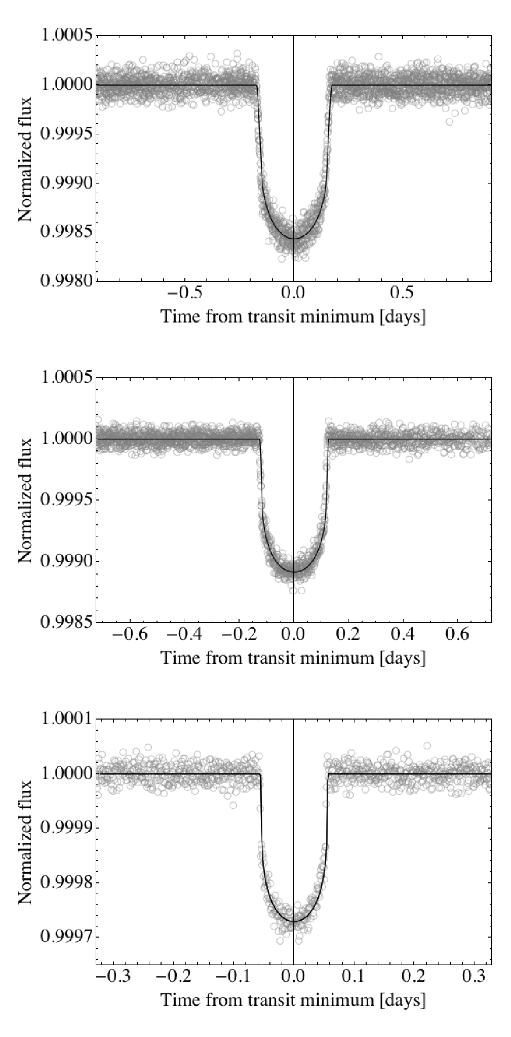
The light curve fits for all three planets are shown in Figure 7 and the derived posteriors are presented in Figure 8. Diagnostics on the mixing and convergence of these MCMC fits are presented in Table 5, all of which indicate reliable results.
As expected, the correct radii, transit epoch and orbital periods were recovered. The derived stellar densities, assuming a circular orbit, were found to be g2/3 cm-2, g2/3 cm-2 and g2/3 cm-2, which clearly deviate significantly from both a common value and the actual stellar density of g2/3 cm-2.
| Planet | # of Accepted | Lowest eff. | Parameter w/ | Highest | Parameter w/ |
|---|---|---|---|---|---|
| MCMC trials | length | lowest eff. len. | Geweke diag. | highest Geweke diag. | |
| KOI-S02.01 | 4808 | 0.0048 | |||
| KOI-S02.02 | 2232 | 0.0074 | |||
| KOI-S02.03 | 1377 | 0.0027 | |||
| n-MAP | 1247 | N/A | N/A |

4.2.3 Results using a-MAP
The analytic approximations from §2.6 may be used to provide lower bounds on combinations of , and via Equation 17, for which we find: (true ), (true ) and (true ). As expected, all of these values are consistent with the true numbers. Further, the significance of each combination being is given by -, - and - respectively, therefore the a-MAP method strongly indicates that the system contains non-zero eccentricities.
4.2.4 Results using n-MAP
Using the n-MAP algorithm described in §3.1, we explored the full 6-dimensional permitted parameter space with MCMC trials. Jump sizes were selected to be 1% for all terms (i.e. , rads). The starting point for the chain was randomly generated until a point with was located. Mixing was checked for as described in §3.6 and the results are reported in Table 5.
The results are shown in Figure 9, after down-sampling to one million trials. The joint posteriors clearly shows the minimum constraints on all three pair-combinations (the white regions in the corner), as derived using a-MAP. We note that the diamonds shown in the joint posteriors of Figure 9 (which represent the true values), consistently lie in densely populated regions, supporting the validity of the MAP technique. The 1D marginalized posteriors yield , and , all consistent with the truth to within 1- except , which is marginally overestimated by 1.3-. Note that the mode tends to overestimate the eccentricity because eccentricity is a positive definite quantity (Lucy & Sweeney, 1971). These results, as with KOI-S01 (§4.1) support the validity of the MAP technique.
In the earlier case of KOI-S01 (§4.1), Figure 6 showed that when the median of posterior (derived using a-MAP) was plotted along with the 2D-marginalized posteriors of versus (derived using n-MAP), there existed excellent agreement on the minimum bound on the pair-combination. In contrast, the KOI-S02 simulation reveals one interesting exception to this pattern, specifically for , as seen in Figure . Here, the median of the posterior (derived using a-MAP) yields whereas visual inpsection of the n-MAP results suggests . Including the a-MAP uncertainties reveals and thus is - deviant from the n-MAP result. Whilst this is not statistically significant (and in fact both the a-MAP and the n-MAP limits are consistent with the truth of ), this is still a large departure relative to the other cases, and may lead the reader to question the origin of this discrepancy.
The reason for the discrepancy can be understood in terms of the approximations made in the original derivation of a-MAP. In §2.4, the derivation of a-MAP includes a step where we assume , allowing us to execute a first-order series expansion. Therefore, one can see that the higher the eccentricity terms, the more a-MAP will depreciate as a reliable approximation. In the KOI-S02 case, the true values of the eccentricity pair-combinations are , and . Consequently, it is clear that is exposed to the highest eccentricity and thus one should expect that a-MAP would be the least reliable for this case. Indeed, this is exactly what is seen, explaining the anomalous behaviour discussed in the previous paragraph. Despite the large pair combined eccentricity of 0.45, it is reassuring that a-MAP still performs quite well, landing to within - of the more sophisticated n-MAP result.

5 Discussion & Conclusions
5.1 Recurring Patterns in MAP
In the 2D posteriors shown in the example systems KOI-SOG, KOI-SOC, KOI-S01 and KOI-S02, it is possible to visually detect some recurring patterns. In this subsection, we will discuss the reason for these patterns.
The most obvious pattern is that the plots tend to exhibit higher densities for . This results in a diagonal high density region extending from the bottom-left to the top-right, getting narrower as it goes up. Why does this happen?
Consider two planets on circular orbits. The light curve derived stellar densities will be identical meaning MAP will find that a system with two circular orbits to be a highly compatible solution. However, it is not the only compatible solution. Consider a MAP realization with and . In this case, a rather broad range of values can reproduce a stellar density which is still equivalent (or within error) to . As increases to higher eccentricities (i.e. as we move along one of the axes), the range of values which can still reproduce such a result diminishes. Consequently, the integrated probability density over all values is small and thus the region becomes a low-probability sector.
Now consider MAP realizations where both and depart from zero. In this case, a situation where and is not grossly different from the case just described where is very large and is zero. Thus these regions tend to be low probability. However, if and both values are large then the range of and values which can reproduce is broader. Thus the integrated probability density becomes larger too. This can be seen be simple inspection of Equation 8. For this reason, a common pattern seen in MAP is the tail extending along the axis.
5.2 MAP in Combination with Other Observables
Multibody Asterodensity Profiling (MAP) can provide constraints on the orbital eccentricity of transiting planets in multiple planet systems without the need for radial velocities, occultations or transit timing variations. However, there may some cases where these observables are available. In such a case, MAP can be combined with these other observables to further refine the constraints on the orbital eccentricities. Our n-MAP technique utilizes an MCMC routine to explore the parameter space of possible orbital eccentricities. This MCMC works by assigning a merit-function to each point and then proceeding via the Metropolis-Hastings rule. Using n-MAP alone, the merit function is:
| (33) |
where is given in Equation 22. If additional observables are available, such as TTVs or RVs then one may simply append the associated merit functions:
| (34) |
Once appended, the n-MAP routine is simply executed as before. In our next paper, we will provide an analysis of this technique on a real transiting planet system featuring both radial velocities and transit timing variations.
5.3 Differences to the Moorhead et al. (2011) Technique
A direct comparison to the method of M11 is not fair because the techniques operate under different conditions and assumptions. Despite this, we will here outline a few differences between the two methods. One advantage of the M11 method is that it works for all transiting planets whereas MAP requires transiting planet in a given system. One advantage of MAP over the M11 technique is that MAP is highly model independent33 3 There is a very weak model dependency in MAP via the adopted limb darkening law, but this can also be fitted for with sufficient signal to noise, assuming only the planets orbit the same star whereas M11 require a value for the stellar radius determined via the more model sensitive route of stellar evolution.
In principle, MAP exploits more information in the light curve than that of the M11 technique. M11 compare the observed transit duration to the maximum theoretical value for a circular orbit; in other words M11 make use of one metric for the duration. Typically, this metric is the transit duration defined as the time for the planet to move from its centre crossing the stellar limb to exitting under the same condition, , since this is independent of the derived planetary radius. In contrast, MAP uses both and the ingress duration, , to derive the light curve derived stellar density assuming a circular orbit, . Thus, it can be appreciated that MAP uses the same information as M11 plus some extra information. In the limit of ignoring this ingress information, the fundamental transit information used by both techniques would be identical.
As a result of M11 negating the ingress duration information, the impact parameter is unresolved. For this reason, M11 adopt the conservative assumption that the limiting case is for . Ford et al. (2008) alternatively discuss how a prior in could be adopted by assuming an isotropic distribution in orbital inclination. In contrast, MAP takes the distribution in from the data itself, essentially characterized by the ingress duration. Due to the conservative assumption made by M11, only transit durations longer than this limiting case can ever be detected. Unlike MAP, this limits the method to detecting eccentric planet transiting near apocentre, the slowest part of the orbit, and also the least likely geometric configuration to detect a transiting planet in (Kane & von Braun, 2008) (this is also pointed out in Tingley & Sackett 2005). This bias, discussed in M11, requires de-biasing any eccentricity statistics deduced and of course reduces the overall sample size since only a subset of eccentric planets are detected. For this reason, we anticipate MAP would provide a more powerful diagnostic of the statistics of eccentric planets, but of course is only applicable in multiple systems.
5.4 Single-body Asterodensity Profiling (SAP)
MAP makes no assumption about the properties of the parent star. For stars with poor characterization, this is an advantage since the stellar properties are frequently subject to unknown systematic uncertainties. However, in some cases the stellar properties are well-characterized and this is information which MAP ignores. An example of this is a star which has been studied with asteroseismology, leading to a highly precise determination of .
Single-body Asterodensity Profiling (SAP) is the logical extension of MAP which can include this information. In this work, we argue in favour of not using SAP due to the frequently unreliable stellar parameters and the strong model dependency of those derived results, which is in stark contrast to the MAP technique. However, for sake of completion we will discuss here a possible implementation of SAP.
In each MCMC trial of the n-MAP algorithm, we create a {} trial vector. This may be used to construct a vector. For a single planet, this would be simply be a 1-dimensional vector: . This value may be used to infer the true stellar density based upon the derived value of via:
| (35) |
For each MCMC trial, we can use the same value of , namely the median of the light curve derived posterior. We now simply define as the number of standard deviations between this trial value of and the empirically determined value of , say :
| (36) |
where we have replaced the 1 subscript (for planet “1”) with to make it a general equation. Clearly for planets we have contributions to the total function from SAP:
| (37) |
This may be combined with the MAP, RV or TTV merit functions as desired to produce finer constraints on the orbital eccentricity.
5.5 Overview
In this work, we have presented a new method to photometrically constrain the orbital eccentricities of transiting planets. The method is only applicable to multiple transiting planet systems and relies on the key assumption that all of the transiting planets orbit the same star. The new method works by comparing the light curve derived stellar density between each planet and thus is dubbed “Multibody Asterodensity Profiling” (MAP). MAP requires no prior information on the star’s properties and thus is highly robust against systematic uncertainties.
MAP constitutes a new observable for which the likelihood of a given orbital configuration can be computed in a -sense. Thus, MAP be be combined with other pieces of information about the eccentricity of the system e.g. transit timing variations, radial velocities, occultations. In this work, we have adopted uniform priors for the orbital eccentricities but more realistic priors based upon dynamics or planet formation can also be invoked (see §3.3).
In its simplest form, MAP can be applied by employing some simple analytic expressions (a-MAP) to deduce the combined eccentricities of two planets (e.g. Equation 11). In this sense, MAP exhibits impressive sensitivity to a system with even a moderate to low eccentricity. For example, for a synthetic system with one planet with (KOI-S01, see §4.1), Q0-Q2 Kepler data can infer a significant eccentricity at the 13- level.
To determine the individual eccentricities require the use of numerical methods, or n-MAP. n-MAP is shown to recover the same constraints for the pair-combined eccentricities as a-MAP does, but additionally provides individual constraints as well as a fuller picture of the inter-relationships between the various eccentricity terms. However, we find MAP is more sensitive to the minimum pair-combined eccentricities than individual terms. Nevertheless, an empricial determination of the posterior for each term is always derivable. The highly model independent nature of MAP means that these posteriors will narrow ad-infinitum as more data and signal-to-noise is accumulated. Further, the application of MAP to dozens of systems raises the potential of discerning truly unbiased statistics on the eccentricity distribution of planets in multiple systems.
Ultimately, MAP has the potential to characterize the eccentricity of the first truly habitable Earth-like planet, which could be found by Kepler. In such a case, the Earth-mass planet will likely be too challenging to detect with radial velocities but MAP will be an ever-present tool provided the photometric time series is of reasonable quality and the system has more than one transiting planet (true of 50% of all transiting planet candidates found by Kepler). In conclusion, MAP offers a method to diagnose both interesting dynamical systems and potentially interesting astrobiological targets too.
The n-MAP algorithm is available as a Fortran 90 script upon request.
Acknowledgments
DMK is supported by the NASA Carl Sagan fellowship scheme. Thanks to G. Bakos for stimulating conversations on this research. WD, JJ and VM would like to thank G. Tinetti for her support and advice during this project. We would like to offer special thanks to our referee, Brandon Tingley, for his insightful comments and suggestions which greatly improved the manuscript.
References
- Bakos et al. (2007) Bakos, G. Á. et al. 2007, ApJ, 670, 826
- Batygin et al. (2009) Batygin, K., Laughlin, G., Meschiari, S., Rivera, E., Vogt, S. & Butler, P. 2009, ApJ, 699, 23
- Borucki et al. (2011) Borucki, W. J. et al. 2011, ApJ, 736, 19
- Brown et al. (2011) Brown, T. M., Latham, D. W., Everett, M. E. & Esquerdo, G. A. 2011, AJ, 142, 112
- Carter et al. (2008) Carter, J. A., Yee, J. C., Eastman, J., Gaudi, B. S. & Winn, J. N. 2008, ApJ, 689, 499
- Catanzarite & Shao (2011) Catanzarite, J. & Shao, M. 2011, ApJ, 738, 151
- Dressing et al. (2010) Dressing, C. D., Spiegel, D. S., Scharf, C. A., Menou, K. & Raymond, S. N. 2010, ApJ, 721, 1295
- Ford et al. (2005) Ford, E. B. 2005, AJ, 129, 1706
- Ford et al. (2008) Ford, E. B., Quinn, S. N. & Veras, D. 2008, ApJ, 678, 1407
- Fressin et al. (2011) Fressin, F. et al. 2011, ApJ, 197, 5
- Geweke (1992) Geweke, J. 1992, Proc. of the Fourth Valencia International Meeting on Bayesian Statistics, ed. J. O. Berger, J. M. Bernando, A. P. Dawid, and A. F. M. Smith, pp. 169-94
- Gladman (1993) Gladman, B. 1993, Icarus, 106, 247
- Holman et al. (2011) Holman, M. J. et al. 2011, Science, 330, 51
- Howard et al. (2010) Howard, A. W. et al. 2010, Science, 330, 653
- Jurić & Tremaine (2008) Jurić, M. & Tremaine, S. 2008, ApJ, 686, 603
- Kane & von Braun (2008) Kane, S. R. & von Braun, K., 2008, ApJ, 689, 492
- Kipping (2008) Kipping, D. M. 2008, MNRAS, 389, 1383
- Kipping (2010) Kipping, D. M. 2010, MNRAS, 407, 301
- Kipping (2011) Kipping, D. M. 2011, PhD thesis, University College London (astro-ph:1105.3189)
- Kipping & Bakos (2011a) Kipping, D. M. & Bakos, G. A. 2011a, ApJ, 730, 50
- Kipping & Bakos (2011b) Kipping, D. M. & Bakos, G. A. 2011b, ApJ, 733, 36
- Kipping & Spiegel (2011) Kipping, D. M. & Spiegel, D. S. 2011, MNRAS Letters, 417, 88
- Kurucz (2006) Kurucz R., 2006, Stellar Model and Associated Spectra (http://kurucz.harvard.edu/grids.html)
- Lissauer et al. (2011) Lissauer, J. J. et al. 2011, Nature, 470, 53
- Lucy & Sweeney (1971) Lucy, L. B. & Sweeney, M. A. 1971, AJ, 76, 544
- Madhusudhan & Seager (2009) Madhusudhan, N. & Seager, 2009, ApJ, 707, 24
- Madhusudhan et al. (2011) Madhusudhan, N. et al. 2011, Nature, 469, 64
- Mandel & Agol (2002) Mandel, K. & Agol, E. 2002, ApJ, 580, L171
- Moorhead et al. (2011) Moorhead, A. V. et al., 2011, ApJ, submitted (astro-ph:1102.0547) (M11)
- Morton & Johnson (2011) Morton, T. D. & Johnson, J. A. 2011, ApJ, submitted (astro-ph:1101.5630)
- Ragozzine & Holman (2010) Ragozzine, D. & Holman, M. J. 2010, arXiv:1006.3727
- Rowe et al. (2011) Rowe, J., Oral presentation 03.02 at the Extreme Solar Systems II Conf., Jackson Hole, Wyoming, 12th Sept 2011
- Seager & Mallén-Ornelas (2003) Seager, S., & Mallén-Ornelas, G., 2003, ApJ, 585, 1038
- Steffen et al. (2010) Steffen, J. H. et al. 2010, ApJ, 725, 1226
- Tegmark et al. (2004) Tegmark, M. et al. 2004, Phys. Rev. D, 69, 103501
- Tingley & Sackett (2005) Tingley, B. & Sackett, P. D., 2005, ApJ, 676, 1011
- Torres et al. (2011) Torres, G. et al. 2011, ApJ, 727, 24
- Valencia et al. (2006) Valencia, D., O’Connell, R. J. & Sasselov, D. 2006, Icarus, 181, 545
- Vogt et al. (2010) Vogt, S. S. et al. 2010, ApJ, 708, 1366
- Williams & Pollard (2002) Williams, D. M. & Pollard, D. 2002, AsB, 1, 61
- Winitzk (2006) Winitzk, S. 2006, “A handy approximation for the error function and its inverse”, lecture note
- Winn (2010) Winn, J. N., 2010, Transits and Occultations, EXOPLANETS, University of Arizona Press; ed: S. Seager
- Wittenmyer et al. (2011) Wittenmyer, R. A., Tinney, C. G., Butler, R. P., O’Toole, S. J., Jones, H. R. A., Carter, B. D., Bailey, J. & Horner, J. 2010, ApJ, submitted (astro-ph:1103:4186)
- Zakamska et al. (2011) Zakamska, N. L., Pan, M. & Ford, E. B. 2011, MNRAS, 410, 1895
Appendix A Further Hypothetical Synthetic Systems
In this appendix, we will present several additional test systems on which we implemented the MAP technique. The systems are control cases uses to ensure we retrieve the correct null results.
A.1 KOI-S0P: Triple System Fit Driven by Uniform Priors Only
A.1.1 Setup
We repeated our analysis of KOI-S01 (see §4.1 for details) but in the second MCMC chain instructed the algorithm to accept all jumps, regardless of the likelihood. This instruction causes the algorithm to produce a result which purely reproduces the initial priors and thus is a useful of way of visualizing what an n-MAP result appears like in the absence of any observational constraints. We dub this system KOI-S0P (for “priors”). The resulting n-MAP posteriors are shown in Figure 10, which clearly reproduce the expected behaviour of uniform priors.

A.2 KOI:S0G: Triple System with Normally Distributed
A.2.1 Setup
For our second control system, we generated three independent distributions for of points each. Each realization is generated with random numbers selected from a normal distribution centred about with standard deviation . This allows us to see the isolated behaviour of MAP without any concern for potential biases from the light curve fitting stage. The resulting posteriors are shown in Figure 11.
The n-MAP MCMC stage stopped when trials had been accepted, using 1% jump sizes for all six free parameters (, , , , , ). Mixing was checked by evaluating the effective lengths of all free parameters from the non-burnt trials, and we found the lowest effective length was 1098 for parameter . In order to keep only points in the figures, we evenly down-sampled the chain to produce the figures. Table 6 summarizes the MCMC diagnostics.
Since all values were selected to be equal, we expect the system to be compatible with a triple-circular orbit system. The n-MAP results indeed agree with this conclusion, as shown in Figure 12. The bulk of the black points (-) land close to circular orbit solutions and the marginalized posteriors of reflect the strong preference towards a low-eccentricity system.
| Planet | # of Accepted | Lowest eff. | Parameter w/ | Highest | Parameter w/ |
|---|---|---|---|---|---|
| MCMC trials | length | lowest eff. len. | Geweke diag. | highest Geweke diag. | |
| KOI-S0G.01 | N/A | N/A | N/A | N/A | |
| KOI-S0G.02 | N/A | N/A | N/A | N/A | |
| KOI-S0G.03 | N/A | N/A | N/A | N/A | |
| n-MAP | 2978 | N/A | N/A |


Both the a-MAP and n-MAP results support the conclusion of a near-circular triple system. The 90% upper limits on the eccentricity were found to be , and .
If we had not used n-MAP but assumed uniform priors in , the probability that (which is a useful rough limit for a habitable world) would be 30% and the probability that would be 70%. Therefore it would be times more likely that the orbit was than otherwise. The same is of course true for and . Using n-MAP these odds ratios become 8.4, 10.4 and 7.8 for , and respectively, demonstrating the extra information we have gained from using n-MAP.
A.3 KOI-S0C: A Perfectly Circular Triple-System
As a final test, we considered a system of three transiting planets, all on circular orbits, denoted KOI-S0C. This system is identical to KOI-S01 (see §4.1) except that for all . The system is generated, noised, re-fitted and treated with a-MAP and n-MAP with precisely the same methodology used on KOI-S01. The MCMC diagnostics are presented in Table 7, which indicate excellent mixing and convergence in all cases.
As expected, the correct radii, transit epoch and orbital periods were easily found in the blind-search. The derived stellar densities, assuming a circular orbit, were found to be g2/3 cm-2, g2/3 cm-2 and g2/3 cm-2 (truth is 1.411 g cm-3).
| Planet | # of Accepted | Lowest eff. | Parameter w/ | Highest | Parameter w/ |
|---|---|---|---|---|---|
| MCMC trials | length | lowest eff. len. | Geweke diag. | highest Geweke diag. | |
| KOI-S0C.01 | 7812 | 0.0034 | |||
| KOI-S0C.02 | 12499 | 0.0017 | |||
| KOI-S0C.03 | 1083 | 0.016 | |||
| n-MAP | 2442 | N/A | N/A |
The n-MAP MCMC stage stopped when trials had been accepted, using 1% jump sizes for all six free parameters (, , , , , ). Mixing was checked by evaluating the effective lengths of all free parameters from the non-burnt trials, and we found the lowest effective length was 1116 for parameter . In order to keep only points in the figures, the chain was again evenly down-sampled.
The results, shown in Figure 13&14, appear similar to those of KOI-S0G (§A.2), which is to be expected given the fact both cases are consistent with a triply-circular system. The results again reflect a range of solutions consistent with circular orbits.


As expected, the MAP results suggest that all three-planets are consistent with a circular orbit. The 90% upper limits on the eccentricity are , and .
If we had not used n-MAP but assumed uniform priors in , the probability that (which is a useful rough limit for a habitable world) would be 30% and the probability that would be 70%. Therfore it would be times more likely that the orbit was than otherwise. The same is of course true for and . Using n-MAP these odds ratios become 5.8, 6.8 and 5.0 for , and respectively, demonstrating the extra information we have gained from using n-MAP.