Inference in Probabilistic Logic Programs with Continuous Random Variables

Muhammad Asiful Islam, C.R. Ramakrishnan, I.V. Ramakrishnan
Dept. of Computer Science
Stony Brook University
Stony Brook NY 11794
{maislam cram ram}@cs.sunysb.edu

Abstract

Probabilistic Logic Programming (PLP), exemplified by Sato and Kameya’s PRISM, Poole’s ICL, Raedt et al’s ProbLog and Vennekens et al’s LPAD, is aimed at combining statistical and logical knowledge representation and inference. However, the inference techniques used in these works rely on enumerating sets of explanations for a query answer. Consequently, these languages permit very limited use of random variables with continuous distributions. In this paper, we present a symbolic inference procedure that uses constraints and represents sets of explanations without enumeration. This permits us to reason over PLPs with Gaussian or Gamma-distributed random variables (in addition to discrete-valued random variables) and linear equality constraints over reals. We develop the inference procedure in the context of PRISM; however the procedure’s core ideas can be easily applied to other PLP languages as well. An interesting aspect of our inference procedure is that PRISM’s query evaluation process becomes a special case in the absence of any continuous random variables in the program. The symbolic inference procedure enables us to reason over complex probabilistic models such as Kalman filters and a large subclass of Hybrid Bayesian networks that were hitherto not possible in PLP frameworks. (To appear in Theory and Practice of Logic Programming)

${{\ignorespaces\begin{array}[c]{[}t]{@{}c@{}}\lx@close@alignment\end{array}\par}}\par\par\par\par$

1 Introduction

Logic Programming (LP) is a well-established language model for knowledge representation based on first-order logic. Probabilistic Logic Programming (PLP) is a class of Statistical Relational Learning (SRL) frameworks [6] which are designed for combining statistical and logical knowledge representation. The semantics of PLP languages is defined based on the semantics of the underlying non-probabilistic logic programs. A large class of PLP languages, including ICL [21], PRISM [26], ProbLog [22] and LPAD [32], have a declarative distribution semantics, which defines a probability distribution over possible models of the program. Operationally, the combined statistical/logical inference is performed based on the proof structures analogous to those created by purely logical inference. In particular, inference proceeds as in traditional LPs except when a random variable’s valuation is used. Use of a random variable creates a branch in the proof structure, one branch for each valuation of the variable. Each proof for an answer is associated with a probability based on the random variables used in the proof and their distributions; an answer’s probability is determined by the probability that at least one proof holds. Since the inference is based on enumerating the proofs/explanations for answers, these languages have limited support for continuous random variables. We address this problem in this paper. A comparison of our work with recent efforts at extending other SRL frameworks to continuous variables appears in Section 2. We provide an inference procedure to reason over PLPs with Gaussian or Gamma-distributed random variables (in addition to discrete-valued ones), and linear equality constraints over values of these continuous random variables. We describe the inference procedure based on extending PRISM with continuous random variables. This choice is based on the following reasons. First of all, the use of explicit random variables in PRISM simplifies the technical development. Secondly, standard statistical models such as Hidden Markov Models (HMMs), Bayesian Networks and Probabilistic Context-Free Grammars (PCFGs) can be naturally encoded in PRISM. Along the same lines, our extension permits natural encodings of Finite Mixture Models (FMMs) and Kalman Filters. Thirdly, PRISM’s inference naturally reduces to the Viterbi algorithm [4] over HMMs, and the Inside-Outside algorithm [16] over PCFGs. The combination of well-defined model theory and efficient inference has enabled the use of PRISM for synthesizing knowledge in sensor networks [28]. It should be noted that, while the technical development in this paper is limited to PRISM, the basic technique itself is applicable to other similar PLP languages such as ProbLog and LPAD (see Section 7).

Our Contribution:

We extend PRISM at the language level to seamlessly include discrete as well as continuous random variables. We develop a new inference procedure to evaluate queries over such extended PRISM programs. • We extend the PRISM language for specifying distributions of continuous random variables, and linear equality constraints over such variables. • We develop a symbolic inference technique to reason with constraints on the random variables. PRISM’s inference technique becomes a special case of our technique when restricted to logic programs with discrete random variables. • These two developments enable the encoding of rich statistical models such as Kalman Filters and a large class of Hybrid Bayesian Networks; and exact inference over such models, which were hitherto not possible in LP and its probabilistic extensions. Note that the technique of using PRISM for in-network evaluation of queries in a sensor network [28] can now be applied directly when sensor data and noise are continuously distributed. Tracking and navigation problems in sensor networks are special cases of the Kalman Filter problem [3]. There are a number of other network inference problems, such as the indoor localization problem, that have been modeled as FMMs [7]. Moreover, our extension permits reasoning over models with finite mixture of Gaussians and discrete distributions (see Section 7). Our extension of PRISM brings us closer to the ideal of finding a declarative basis for programming in the presense of noisy data. The rest of this paper is organized as follows. We begin with a review of related work in Section 2, and describe the PRISM framework in detail in Section 3. We introduce the extended PRISM language and the symbolic inference technique for the extended language in Section 5. In section 6 we show the use of this technique on an example encoding of the Kalman Filter. We conclude in Section 7 with a discussion on extensions to our inference procedure.

2 Related Work

Over the past decade, a number of Statistical Relational Learning (SRL) frameworks have been developed, which support modeling, inference and/or learning using a combination of logical and statistical methods. These frameworks can be broadly classified as statistical-model-based or logic-based, depending on how their semantics is defined. In the first category are frameworks such as Bayesian Logic Programs (BLPs) [14], Probabilistic Relational Models (PRMs) [5], and Markov Logic Networks (MLNs) [23], where logical relations are used to specify a model compactly. A BLP consists of a set of Bayesian clauses (constructed from Bayesian network structure), and a set of conditional probabilities (constructed from CPTs of Bayesian network). PRMs encodes discrete Bayesian Networks with Relational Models/Schemas. An MLN is a set of formulas in first order logic associated with weights. The semantics of a model in these frameworks is given in terms of an underlying statistical model obtained by expanding the relations. Inference in SRL frameworks such as PRISM [26], Stochastic Logic Programs (SLP) [17], Independent Choice Logic (ICL) [21], and ProbLog [22] is primarily driven by query evaluation over logic programs. In SLP, clauses of a logic program are annotated with probabilities, which are then used to associate probabilities with proofs (derivations in a logic program). ICL [20] consists of definite clauses and disjoint declarations of the form

disjoint([h_{1}:p_{1},...,h_{n}:p_{n}])

that specifies a probability distribution over the hypotheses (i.e.,

\{h_{1},..,h_{n}\}

). Any probabilistic knowledge representable in a discrete Bayesian network can be represented in this framework. While the language model itself is restricted (e.g., ICL permits only acyclic clauses), it had declarative distribution semantics. This semantic foundation was later used in other frameworks such as PRISM and ProbLog. CP-Logic [31] is a logical language to represent probabilistic causal laws, and its semantics is equivalent to probability distribution over well-founded models of certain logic programs. Specifications in LPAD [32] resemble those in CP-Logic: probabilistic predicates are specified with disjunctive clauses, i.e. clauses with multiple disjunctive consequents, with a distribution defined over the consequents. LPAD has a distribution semantics, and a proof-based operational semantics similar to that of PRISM. ProbLog specifications annotate facts in a logic program with probabilities. In contrast to SLP, ProbLog has a distribution semantics and a proof-based operational semantics. PRISM (discussed in detail in the next section), LPAD and ProbLog are equally expressive. PRISM uses explicit random variables and a simple inference but restricted procedure. In particular, PRISM demands that the set of proofs for an answer are pairwise mutually exclusive, and that the set of random variables used in a single proof are pairwise independent. The inference procedures of LPAD and ProbLog lift these restrictions. SRL frameworks that are based primarily on statistical inference, such as BLP, PRM and MLN, were originally defined over discrete-valued random variables, and have been naturally extended to support a combination of discrete and continuous variables. Continuous BLP [15] and Hybrid PRM [19] extend their base models by using Hybrid Bayesian Networks [18]. Hybrid MLN [33] allows description of continuous properties and attributes (e.g., the formula

\mbox{length\/}(x)=5

with weight

w

) deriving MRFs with continuous-valued nodes (e.g., length(a) for a grounding of

x

, with mean

5

and standard deviation

1/\sqrt{2w}

). In contrast to BLP, PRM and MLN, SRL frameworks that are primarily based on logical inference offer limited support for continuous variables. In fact, among such frameworks, only ProbLog has been recently extended with continuous variables. Hybrid ProbLog [8] extends Problog by adding a set of continuous probabilistic facts (e.g.,

(X_{i},\phi_{i})::f_{i}

, where

X_{i}

is a variable appearing in atom

f_{i}

, and

\phi_{i}

denotes its Gaussian density function). It adds three predicates namely below, above, ininterval to the background knowledge to process values of continuous facts. A ProbLog program may use a continuous random variable, but further processing can be based only on testing whether or not the variable’s value lies in a given interval. As a consequence, statistical models such as Finite Mixture Models can be encoded in Hybrid ProbLog, but others such as certain classes of Hybrid Bayesian Networks (with continuous child with continuous parents) and Kalman Filters cannot be encoded. The extension to PRISM described in this paper makes the framework general enough to encode such statistical models. More recently, [9] introduced a sampling based approach for (approximate) probabilistic inference in a ProbLog-like language that combines continuous and discrete random variables. The inference algorithm uses forward chaining and rejection sampling. The language permits a large class of models where discrete and continuous variables may be combined without restriction. In contrast, we propose an exact inference algorithm with a more restrictive language, but ensure that inference matches the complexity of specialized inference algorithms for important classes of statistical models (e.g., Kalman filters).

3 Background: an overview of PRISM

PRISM programs have Prolog-like syntax (see Fig. 1). In a PRISM program the msw relation (“multi-valued switch”) has a special meaning: msw(X,I,V) says that V is the outcome of the I-th instance from a family X of random processes¹¹ 1 Following PRISM, we often omit the instance number in an msw when a program uses only one instance from a family of random processes.. The set of variables

\{\mathtt{V}_{i}\mid\mathtt{msw(}p,i,\mathtt{V}_{i}\mathtt{)}\}

are i.i.d. for a given random process

p

. The distribution parameters of the random variables are specified separately. The program in Fig. 1 encodes a Hidden Markov Model (HMM) in PRISM. Refer to caption

Figure 1: PRISM program for an HMM The set of observations is encoded as facts of predicate obs, where obs(I,V) means that value V was observed at time I. In the figure, the clause defining hmm says that T is the N-th state if we traverse the HMM starting at an initial state S (itself the outcome of the random process init). In hmm_part(I, N, S, T), S is the I-th state, T is the N-th state. The first clause of hmm_part defines the conditions under which we go from the I-th state S to the I+1-th state NextS. Random processes trans(S) and emit(S) give the distributions of transitions and emissions, respectively, from state S. The meaning of a PRISM program is given in terms of a distribution semantics [26, 27]. A PRISM program is treated as a non-probabilistic logic program over a set of probabilistic facts, the msw relation. An instance of the msw relation defines one choice of values of all random variables. A PRISM program is associated with a set of least models, one for each msw relation instance. A probability distribution is then defined over the set of models, based on the probability distribution of the msw relation instances. This distribution is the semantics of a PRISM program. Note that the distribution semantics is declarative. For a subclass of programs, PRISM has an efficient procedure for computing this semantics based on OLDT resolution [30]. Inference in PRISM proceeds as follows. When the goal selected at a step is of the form msw(X,I,Y), then Y is bound to a possible outcome of a random process X. Thus in PRISM, derivations are constructed by enumerating the possible outcomes of each random variable. The derivation step is associated with the probability of this outcome. If all random processes encountered in a derivation are independent, then the probability of the derivation is the product of probabilities of each step in the derivation. If a set of derivations are pairwise mutually exclusive, the probability of the set is the sum of probabilities of each derivation in the set. PRISM’s evaluation procedure is defined only when the independence and exclusiveness assumptions hold. Finally, the probability of an answer is the probability of the set of derivations of that answer.

4 Extended PRISM

Support for continuous variables is added by modifying PRISM’s language in two ways. We use the msw relation to sample from discrete as well as continuous distributions. In PRISM, a special relation called values is used to specify the ranges of values of random variables; the probability mass functions are specified using set_sw directives. In our extension, we extend the set_sw directives to specify probability density functions as well. For instance, set_sw(r, norm(Mu,Var)) specifies that outcomes of random processes r have Gaussian distribution with mean Mu and variance Var²² 2 The technical development in this paper considers only univariate Gaussian variables; see Discussions section on a discussion on how multivariate Gaussian as well as other continuous distributions are handled.. Parameterized families of random processes may be specified, as long as the parameters are discrete-valued. For instance, set_sw(w(M), norm(Mu,Var)) specifies a family of random processes, with one for each value of M. As in PRISM, set_sw directives may be specified programmatically; for instance, in the specification of w(M), the distribution parameters may be computed as functions of M. Additionally, we extend PRISM programs with linear equality constraints over reals. Without loss of generality, we assume that constraints are written as linear equalities of the form

Y=a_{1}*X_{1}+\ldots+a_{n}*X_{n}+b

where

a_{i}

and

b

are all floating-point constants. The use of constraints enables us to encode Hybrid Bayesian Networks and Kalman Filters as extended PRISM programs. In the following, we use Constr to denote a set (conjunction) of linear equality constraints. We also denote by

\overline{X}

a vector of variables and/or values, explicitly specifying the size only when it is not clear from the context. This permits us to write linear equality constraints compactly (e.g.,

Y=\overline{a}\cdot\overline{X}+b

). Encoding of Kalman Filter specifications uses linear constraints and closely follows the structure of the HMM specification, and is shown in Section 6.

Distribution Semantics:

We extend PRISM’s distribution semantics for continuous random variables as follows. The idea is to construct a probability space for the msw definitions (called probabilistic facts in PRISM) and then extend it to a probability space for the entire program using least model semantics. Sample space for the probabilistic facts is constructed from those of discrete and continuous random variables. The sample space of a continuous random variable is the set of real numbers,

\Re

. The sample space of a set of random variables is a Cartesian product of the sample spaces of individual variables. We complete the definition of a probability space for

N

continuous random variables by considering the Borel

\sigma

-algebra over

\Re^{N}

, and defining a Lebesgue measure on this set as the probability measure. Lifting the probability space to cover the entire program needs one significant step. We use the least model semantics of constraint logic programs [13] as the basis for defining the semantics of extended PRISM programs. A point in the sample space is an arbitrary interpretation of the program, with its Herbrand universe and

\Re

as the domain of interpretation. For each sample, we distinguish between the interpretation of user-defined predicates and probabilistic facts. Note that only the probabilistic facts have probabilistic behavior in PRISM; the rest of a model is defined in terms of logical consequence. Hence, we can define a probability measure over a set of sample points by using the measure defined for the probabilistic facts alone. The semantics of an extended PRISM program is thus defined as a distribution over its possible models.

5 Inference

Recall that PRISM’s inference explicitly enumerates outcomes of random variables in derivations. The key to inference in the presence of continuous random variables is avoiding enumeration by representing the derivations and their attributes symbolically. A single step in the construction of a symbolic derivation is defined below.

Definition 1 (Symbolic Derivation)

A goal

G

directly derives goal

G^{\prime}

, denoted

G\rightarrow G^{\prime}

, if: PCR:

G=q_{1}(\overline{X_{1}}),G_{1}

, and there exists a clause in the program,

q_{1}(\overline{Y}):-r_{1}(\overline{Y_{1}}),r_{2}(\overline{Y_{2}}),\ldots,r_{m}(\overline{Y_{m}})

, such that

\theta=\mbox{mgu }(q_{1}(\overline{X_{1}}),q_{1}(\overline{Y}))

; then,

G^{\prime}=(r_{1}(\overline{Y_{1}}),r_{2}(\overline{Y_{2}}),\ldots,r_{m}(\overline{Y_{m}}),G_{1})\theta

; MSW:

G=\mathtt{msw}(\mbox{rv }(\overline{X}),Y),G_{1}

: then

G^{\prime}=G_{1}

; CONS:

G=\mbox{Constr\/},G_{1}

and Constr is satisfiable: then

G^{\prime}=G_{1}

. A symbolic derivation of

G

is a sequence of goals

G_{0},G_{1},\ldots

such that

G=G_{0}

and, for all

i\geq 0

G_{i}\rightarrow G_{i+1}

. We only consider successful derivations, i.e., the last step of a derivation resolves to an empty clause. Note that the traditional notion of derivation in a logic program coincides with that of symbolic derivation when the selected subgoal (literal) is not an msw or a constraint. When the selected subgoal is an msw, PRISM’s inference will construct the next step by enumerating the values of the random variable. In contrast, symbolic derivation skips msw’s and constraints and continues with the remaining subgoals in a goal. The effect of these constructs is computed by associating (a) variable type information and (b) a success function (defined below) with each goal in the derivation. The symbolic derivation for the goal widget(X) over the program in Example 1 is shown in Fig. 2(b).

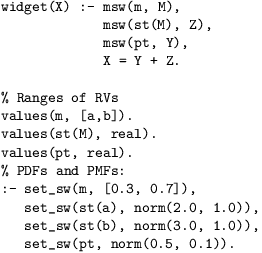(a) Mixture model program

(b) Symbolic derivation for goal widget(X)

Figure 2: Finite Mixture Model Program and Symbolic Derivation

Example 1

Consider a factory with two machines a and b. Each machine produces a widget structure and then the structure is painted with a color. In the program Fig. 2(a), msw(m, M) chooses either machine a or b, msw(st(M), Z) gives the cost Z of a product structure, msw(pt, Y) gives the cost Y of painting, and finally X = Y + Z returns the price of a painted widget X.

\sqcap

\sqcup

(a) Example program

(b) Symbolic derivation for goal q(Y)

Figure 3: Symbolic derivation

Example 2

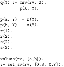
This example illustrates how symbolic derivation differs from traditional logic programming derivation. Fig. 3(b) shows the symbolic derivation for goal

q(Y)

in Fig. 3(a). Notice that the symbolic derivation still makes branches in the derivation tree for various logic definitions and outcomes. But the main difference with traditional logic derivation is that it skips msw and Constr definitions, and continues with the remaining subgoals in a goal.

\sqcap

\sqcup

Success Functions:

Goals in a symbolic derivation may contain variables whose values are determined by msw’s appearing subsequently in the derivation. With each goal

G_{i}

in a symbolic derivation, we associate a set of variables,

V(G_{i})

, that is a subset of variables in

G_{i}

. The set

V(G_{i})

is such that the variables in

V(G_{i})

subsequently appear as parameters or outcomes of msw’s in some subsequent goal

G_{j}

j\geq i

. We can further partition

V

into two disjoint sets,

V_{c}

and

V_{d}

, representing continuous and discrete variables, respectively. The sets

V_{c}

and

V_{d}

are called the derivation variables of

G_{i}

, defined below.

Definition 2 (Derivation Variables)

Let

G\rightarrow G^{\prime}

such that

G^{\prime}

is derived from

G

using: PCR: Let

\theta

be the mgu in this step. Then

V_{c}(G)

and

V_{d}(G)

are the largest sets of variables in

G

such that

V_{c}(G)\theta\subseteq V_{c}(G^{\prime})

and

V_{d}(G)\theta\subseteq V_{d}(G^{\prime})

. MSW: Let

G=\mbox{msw}(\mbox{rv }(\overline{X}),Y),G^{\prime}

. Then

V_{c}(G)

and

V_{d}(G)

are the largest sets of variables in

G

such that

V_{c}(G)\subseteq V_{c}(G^{\prime})\cup\{Y\}

, and

V_{d}(G)\subseteq V_{d}(G^{\prime})\cup\overline{X}

Y

is continuous, otherwise

V_{c}(G)\subseteq V_{c}(G^{\prime})

, and

V_{d}(G)\subseteq V_{d}(G^{\prime})\cup\overline{X}\cup\{Y\}

. CONS: Let

G=\mbox{Constr\/},G^{\prime}

. Then

V_{c}(G)

and

V_{d}(G)

are the largest sets of variables in

G

such that

V_{c}(G)\subseteq V_{c}(G^{\prime})\cup\mbox{vars\/}(\mbox{Constr\/})

, and

V_{d}(G)\subseteq V_{d}(G^{\prime})

. Given a goal

G_{i}

in a symbolic derivation, we can associate with it a success function, which is a function from the set of all valuations of

V(G_{i})

[0,1]

. Intuitively, the success function represents the probability that the symbolic derivation represents a successful derivation for each valuation of

V(G_{i})

Representation of success functions:

Given a set of variables

\mathbf{V}

, let

\mathbf{C}

denote the set of all linear equality constraints over reals using

\mathbf{V}

. Let

\mathbf{L}

be the set of all linear functions over

\mathbf{V}

with real coefficients. Let

\mathcal{N}_{X}(\mu,\sigma^{2})

be the PDF of a univariate Gaussian distribution with mean

\mu

and variance

\sigma^{2}

, and

\delta_{x}(X)

be the Dirac delta function which is zero everywhere except at

x

and integration of the delta function over its entire range is 1. Expressions of the form

k*\prod_{l}\delta_{v}(V_{l})\prod_{i}\mathcal{N}_{f_{i}}

, where

k

is a non-negative real number and

f_{i}\in\mathbf{L}

, are called product PDF (PPDF) functions over

\mathbf{V}

. We use

\phi

(possibly subscripted) to denote such functions. A pair

\langle\phi,C\rangle

where

C\subseteq\mathbf{C}

is called a constrained PPDF function. A sum of a finite number of constrained PPDF functions is called a success function, represented as

\sum_{i}\langle\phi_{i},C_{i}\rangle

. We use

C_{i}(\psi)

to denote the constraints (i.e.,

C_{i}

) in the

i^{th}

constrained PPDF function of success function

\psi

; and

D_{i}(\psi)

to denote the

i^{th}

PPDF function of

\psi

Success functions of base predicates:

The success function of a constraint

C

\langle 1,C\rangle

. The success function of true is

\langle 1,\mbox{true\/}\rangle

. The PPDF component of

\mathtt{msw}(\mbox{rv }(\overline{X}),Y)

’s success function is the probability density function of rv ’s distribution if rv is continuous, and its probability mass function if rv is discrete; its constraint component is true. Refer to caption

Figure 4: Success Functions

Example 3

The success function

\psi_{1}

of msw(m,M) for the program in Example 1 is such that

\psi_{1}=0.3\delta_{a}(M)+0.7\delta_{b}(M)

. Note that we can represent the success function using tables, where each table row denotes discrete random variable valuations. For example, the above success function can be represented as Fig. 4a. Thus instead of using delta functions, we often omit it in examples and represent success functions using tables. Fig. 4b represents the success function of msw(st(M), Z) for the program in Example 1. Similarly, the success function

\psi_{3}

of msw(pt, Y) for the program in Example 1 is

\psi_{3}=\mathcal{N}_{Y}(0.5,0.1)

. Finally, the success function

\psi_{4}

of X = Y + Z for the program in Example 1 is

\psi_{4}=\langle 1,\mbox{{\color[rgb]{0,0,1}$X=Y+Z$}}\rangle

\sqcap

\sqcup

Success functions of user-defined predicates:

G\rightarrow G^{\prime}

is a step in a derivation, then the success function of

G

is computed bottom-up based on the success function of

G^{\prime}

. This computation is done using join and marginalize operations on success functions.

Definition 3 (Join)

Let

\psi_{1}=\sum_{i}\langle D_{i},C_{i}\rangle

and

\psi_{2}=\sum_{j}\langle D_{j},C_{j}\rangle

be two success functions, then join of

\psi_{1}

and

\psi_{2}

represented as

\psi_{1}*\psi_{2}

is the success function

\sum_{i,j}\langle D_{i}D_{j},C_{i}\wedge C_{j}\rangle

Example 4

Let Fig. 5(a) and 5(b) represent the success functions

\psi_{msw(m,M)}(M)

and

\psi_{G_{3}}(X,Y,Z,M)

respectively.

(a)

(b)

(c)

Figure 5: Join of Success Functions Then Fig. 5(c) shows the join of

\psi_{msw(m,M)}(M)

and

\psi_{G_{3}}(X,Y,Z,M)

\sqcap

\sqcup

Note that we perform a simplification of success functions after the join operation. We eliminate any PPDF term in

\psi

which is inconsistent w.r.t. delta functions. For example,

\delta_{a}(M)\delta_{b}(M)=0

M

can not be both

a

and

b

at the same time. Given a success function

\psi

for a goal

G

, the success function for

\exists X.\ G

is computed by the marginalization operation. Marginalization w.r.t. a discrete variable is straightforward and omitted. Below we define marginalization w.r.t. continuous variables in two steps: first rewriting the success function in a projected form and then doing the required integration. The goal of projection is to eliminate any linear constraint on

V

, where

V

is the continuous variable to marginalize over. The projection operation involves finding a linear constraint (i.e.,

V=\overline{a}\cdot\overline{X}+b

) on

V

and replacing all occurrences of

V

in the success function by

\overline{a}\cdot\overline{X}+b

Definition 4 (Projection)

Projection of a success function

\psi

w.r.t. a continuous variable

V

, denoted by

\psi\downarrow_{V}

, is a success function

\psi^{\prime}

such that

\forall i.\ D_{i}(\psi^{\prime})=D_{i}(\psi)[\overline{a}\cdot\overline{X}+b/V]

; and

C_{i}(\psi^{\prime})=(C_{i}(\psi)-C_{ip})[\overline{a}\cdot\overline{X}+b/V]

,
where

C_{ip}

is a linear constraint (

V=\overline{a}\cdot\overline{X}+b

) on

V

C_{i}(\psi)

and

t[s/x]

denotes replacement of all occurrences of

x

t

s

. Note that the replacement of

V

\overline{a}\cdot\overline{X}+b

in PDFs and linear constraints does not alter the general form of a success function. Thus projection returns a success function. Notice that if

\psi

does not contain any linear constraint on

V

, then the projected form remains the same.

Example 5

Let

\psi_{1}=\langle 0.3\mathcal{N}_{Z}(2.0,1.0).\mathcal{N}_{Y}(0.5,0.1),\mbox{{\color[rgb]{0,0,1}$X=Y+Z$}}\rangle

represent a success function. Then projection of

\psi_{1}

w.r.t.

Y

yields

\psi_{1}\downarrow_{Y}=0.3\mathcal{N}_{Z}(2.0,1.0).\mathcal{N}_{X-Z}(0.5,0.1).

(1) Notice that

Y

is replaced by

X-Z

\sqcap

\sqcup

Proposition 1

Integration of a PPDF function with respect to a variable

V

is a PPDF function, i.e.,

\displaystyle\alpha\int^{\infty}_{-\infty}\prod_{k=1}^{m}\mathcal{N}_{(\overline{a_{k}}\cdot\overline{X_{k}}+b_{k})}(\mu_{k},\sigma^{2}_{k})dV=\alpha^{\prime}\prod_{l=1}^{m^{\prime}}\mathcal{N}_{(\overline{a^{\prime}_{l}}\cdot\overline{X^{\prime}_{l}})+b^{\prime}_{l}}(\mu^{\prime}_{l},\sigma^{\prime 2}_{l})

where

V\in\overline{X_{k}}

and

V\not\in\overline{X^{\prime}_{l}}

. For example,

\displaystyle\int^{\infty}_{-\infty}\mathcal{N}_{a_{1}V-X_{1}}(\mu_{1},\sigma_{1}^{2}).\mathcal{N}_{a_{2}V-X_{2}}(\mu_{2},\sigma_{2}^{2})dV

\displaystyle=\mathcal{N}_{a_{2}X_{1}-a_{1}X_{2}}(a_{1}\mu_{2}-a_{2}\mu_{1},a_{2}^{2}\sigma_{1}^{2}+a_{1}^{2}\sigma_{2}^{2}).

(2) Here

X_{1},X_{2}

are linear combinations of variables (except

V

). A proof of the proposition is presented in Section 8.

Definition 5 (Integration)

Let

\psi

be a success function that does not contain any linear constraints on

V

. Then integration of

\psi

with respect to

V

, denoted by

\oint_{V}\psi

is a success function

\psi^{\prime}

such that

\forall i.D_{i}(\psi^{\prime})=\int D_{i}(\psi)dV

. It is easy to see (using Proposition 1) that the integral of success functions are also success functions. Note that if

\psi

does not contain any PDF on

V

, then the integrated form remains the same.

Example 6

Let

\psi_{2}=0.3\mathcal{N}_{Z}(2.0,1.0).\mathcal{N}_{X-Z}(0.5,0.1)

represent a success function. Then integration of

\psi_{2}

w.r.t.

Z

yields

\displaystyle\oint_{Z}\psi_{2}

\displaystyle=\int 0.3\mathcal{N}_{Z}(2.0,1.0).\mathcal{N}_{X-Z}(0.5,0.1)dZ

\displaystyle=0.3\mathcal{N}_{X}(2.5,1.1).\textrm{ (using Equation~\ref{intgr-eq})}

Definition 6 (Marginalize)

Marginalization of a success function

\psi

with respect to a variable

V

, denoted by

\mathbb{M}(\psi,V)

, is a success function

\psi^{\prime}

such that

\displaystyle\psi^{\prime}

\displaystyle=\oint_{V}\psi\downarrow_{V}

We overload

\mathbb{M}

to denote marginalization over a set of variables, defined such that

\mathbb{M}(\psi,\{V\}\cup\overline{X})=\mathbb{M}(\mathbb{M}(\psi,V),\overline{X})

and

\mathbb{M}(\psi,\{\})=\psi

Proposition 2

The set of all success functions is closed under join and marginalize operations. The success function for a derivation is defined as follows.

Definition 7 (Success function of a goal)

The success function of a goal

G

, denoted by

\psi_{G}

, is computed based on the derivation

G\rightarrow G^{\prime}

\psi_{G}=\left\{\begin{array}[]{ll}\sum_{G^{\prime}}\mathbb{M}(\psi_{G^{\prime}},V(G^{\prime})-V(G))&\text{for all program clause resolution $G\rightarrow G^{\prime}$}\\ \psi_{msw(rv(\overline{X}),Y)}*\psi_{G^{\prime}}&\text{if $G=\mbox{msw}(\mbox{rv }(\overline{X}),Y),G^{\prime}$}\\ \psi_{Constr}*\psi_{G^{\prime}}&\text{if $G=Constr,G^{\prime}$}\\ \end{array}\right.

Note that the above definition carries PRISM’s assumption that an instance of a random variable occurs at most once in any derivation. In particular, the PCR step marginalizes success functions w.r.t. a set of variables; the valuations of the set of variables must be mutually exclusive for correctness of this step. The MSW step joins success functions; the goals joined must use independent random variables for the join operation to correctly compute success functions in this step.

Example 7

Fig. 2(b) shows the symbolic derivation for the goal widget(X) over the mixture model program in Example 1. The success function of goal

G_{5}

\psi_{G_{5}}(X,Y,Z)=\langle 1,\mbox{{\color[rgb]{0,0,1}$X=Y+Z$}}\rangle

\displaystyle\psi_{G_{4}}(X,Y,Z)=\psi_{msw(pt,Y)}(Y)*\psi_{G_{5}}(X,Y,Z)=\langle\mathcal{N}_{Y}(0.5,0.1),\mbox{{\color[rgb]{0,0,1}$X=Y+Z$}}\rangle.

The success function of goal

G_{3}

\psi_{msw(st(M),Z)}(Z)*\psi_{G_{4}}(X,Y,Z)

(Fig. 5(b)). Then join of

\psi_{msw(m,M)}(M)

and

\psi_{G_{3}}(X,Y,Z,M)

yields the success function in Fig. 5(c) (see Example 4). Finally,

\psi_{G_{1}}(X)=\mathbb{M}(\psi_{G_{2}}(X,Y,Z,M),\{M,Y,Z\})

. First we marginalize

\psi_{G_{2}}(X,Y,Z,M)

w.r.t.

M

\displaystyle\psi_{G_{2}}^{\prime}

\displaystyle=\mathbb{M}(\psi_{G_{2}},M)=\oint_{M}\psi_{G_{2}}\downarrow_{M}

\displaystyle=\langle 0.3\mathcal{N}_{Z}(2.0,1.0).\mathcal{N}_{Y}(0.5,0.1),\mbox{{\color[rgb]{0,0,1}$X=Y+Z$}}\rangle

\displaystyle+\langle 0.7\mathcal{N}_{Z}(3.0,1.0).\mathcal{N}_{Y}(0.5,0.1),\mbox{{\color[rgb]{0,0,1}$X=Y+Z$}}\rangle.

Next we marginalize the above success function w.r.t.

Y

\displaystyle\psi_{G_{2}}^{\prime\prime}

\displaystyle=\mathbb{M}(\psi_{G_{2}}^{\prime},Y)=\oint_{Y}\psi_{G_{2}}^{\prime}\downarrow_{Y}

\displaystyle=0.3\mathcal{N}_{Z}(2.0,1.0).\mathcal{N}_{X-Z}(0.5,0.1)+0.7\mathcal{N}_{Z}(3.0,1.0).\mathcal{N}_{X-Z}(0.5,0.1).

Finally, we marginalize the above function over variable

Z

to get

\psi_{G_{1}}(X)

\displaystyle\psi_{G_{1}}(X)=\mathbb{M}(\psi_{G_{2}}^{\prime\prime},Z)=\oint_{Z}\psi_{G_{2}}^{\prime\prime}\downarrow_{Z}=0.3\mathcal{N}_{X}(2.5,1.1)+0.7\mathcal{N}_{X}(3.5,1.1).

Example 8

In this example, we compute success function of goal

q(Y)

in Example 2. Fig. 3(b) shows the symbolic derivation for goal

q(Y)

. Success function of

r(Y)

\delta_{1}(Y)+\delta_{2}(Y)

, and success function of

s(Y)

\delta_{2}(Y)+\delta_{3}(Y)

. Similarly, success function of

p(X,Y)

\delta_{a}(X)(\delta_{1}(Y)+\delta_{2}(Y))+\delta_{b}(X)(\delta_{2}(Y)+\delta_{3}(Y))

. Now

\displaystyle\psi_{q(Y)}

\displaystyle=\mathbb{M}(\psi_{msw(rv,X)}*\psi_{p(X,Y)},X)

Success function of

msw(rv,X)

0.3\delta_{a}(X)+0.7\delta_{b}(X)

. Join of

\psi_{msw(rv,X)}

and

\psi_{p(X,Y)}

yields

0.3\delta_{a}(X)(\delta_{1}(Y)+\delta_{2}(Y))+0.7\delta_{b}(X)(\delta_{2}(Y)+\delta_{3}(Y))

. Finally,

\psi_{q(Y)}=0.3(\delta_{1}(Y)+\delta_{2}(Y))+0.7(\delta_{2}(Y)+\delta_{3}(Y))

. When

Y=1

, only

p(a,1)

is true. Thus

\psi_{q(1)}=0.3

. On the other hand,

\psi_{q(2)}=1.0

as both

p(a,2)

and

p(b,2)

are true when Y=2. Similarly,

\psi_{q(3)}=0.7

\sqcap

\sqcup

Complexity:

Let

S_{i}

denote the number of constrained PPDF terms in

\psi_{i}

;

P_{i}

denote the maximum number of product terms in any PPDF function in

\psi_{i}

; and

Q_{i}

denote the maximum size of a constraint set (

C_{i}

) in

\psi_{i}

. The time complexity of the two basic operations used in constructing a symbolic derivation is as follows.

Proposition 3 (Time Complexity)

The worst-case time complexity of

\mbox{Join\/}(\psi_{i},\psi_{j})

O(S_{i}*S_{j}*(P_{i}*P_{j}+Q_{i}*Q_{j}))

. The worst-case time complexity of

\mathbb{M}(\psi_{g},V)

O(S_{g}*P_{g})

when

V

is discrete and

O(S_{g}*(P_{g}+Q_{g}))

when

V

is continuous. Note that when computing the success function of a goal in a derivation, the join operation is limited to joining the success function of a single msw or a single constraint set to the success function of a goal, and hence the parameters

S_{i},P_{i}

, and

Q_{i}

are typically small. The complexity of the size of success functions is as follows.

Proposition 4 (Success Function Size)

For a goal

G

and its symbolic derivation, the following hold: 1. The maximum number of product terms in any PPDF function in

\psi_{G}

is linear in

|V_{c}(G)|

, the number of continuous variables in

G

. 2. The maximum size of a constraint set in a constrained PPDF function in

\psi_{G}

is linear in

|V_{c}(G)|

. 3. The maximum number of constrained PPDF functions in any entry of

\psi_{G}

is potentially exponential in the number of discrete random variables in the symbolic derivation. The number of product terms and the size of constraint sets are hence independent of the length of the symbolic derivation. Note that for a program with only discrete random variables, there may be exponentially fewer symbolic derivations than concrete derivations. The compactness is only in terms of number of derivations and not the total size of the representations. In fact, for programs with only discrete random variables, there is a one-to-one correspondence between the entries in the tabular representation of success functions and PRISM’s answer tables. For such programs, it is easy to show that the time complexity of the inference algorithm presented in this paper is same as that of PRISM.

Correctness of the Inference Algorithm:

The technically complex aspect of correctness is the closure of the set of success functions w.r.t. join and marginalize operations. Proposition 1 and 2 state these closure properties. Definition 7 represents the inference algorithm for computing the success function of a goal. The distribution of a goal is formally defined in terms of the distribution semantics of extended PRISM programs and is computed using the inference algorithm.

Theorem 5

The success function of a goal computed by the inference algorithm represents the distribution of the answer to that goal.

Proof:

Correctness w.r.t. distribution semantics follows from the definition of join and marginalize operations, and PRISM’s independence and exclusiveness assumptions. We prove this by induction on derivation length

n

. For

n=1

, the definition of success function for base predicates gives a correct distribution. Now let’s assume that for a derivation of length

n

, our inference algorithm computes valid distribution. Let’s assume that

G^{\prime}

has a derivation of length

n

and

G\rightarrow G^{\prime}

. Thus

G

has a derivation of length

n+1

. We show that the success function of

G

represents a valid distribution. We compute

\psi_{G}

using Definition 7 and it carries PRISM’s assumption that an instance of a random variable occurs at most once in any derivation. More specifically, the PCR step marginalizes

\psi_{G^{\prime}}

w.r.t. a set of variables

V(G^{\prime})-V(G)

. Since according to PRISM’s exclusiveness assumption the valuations of the set of variables are mutually exclusive, the marginalization operation returns a valid distribution. Analogously, the MSW/CONS step joins success functions, and the goals joined use independent random variables (following PRISM’s assumption) for the join operation to correctly compute

\psi_{G}

in this step. Thus

\psi_{G}

represents a valid distribution.

6 Illustrative Example

kf(N, T) :-
  msw(init, S),
  kf_part(0, N, S, T).

kf_part(I, N, S, T) :-
  I < N, NextI is I+1,
  trans(S, I, NextS),
  emit(NextS, NextI, V),
  obs(NextI, V),
  kf_part(NextI, N, NextS, T).

kf_part(I, N, S, T) :-
  I=N, T=S.

trans(S, I, NextS) :-
  msw(trans_err, I, E),
  NextS = S + E.

emit(NextS, I, V) :-
  msw(obs_err, I, X),
  V = NextS + X.

Figure 6: Logic program for Kalman Filter In this section, we model Kalman filters [25] using logic programs. The model describes a random walk of a single continuous state variable

S_{t}

with noisy observation

V_{t}

. The initial state distribution is assumed to be Gaussian with mean

\mu_{0}

, and variance

\sigma_{0}^{2}

. The transition and sensor models are Gaussian noises with zero means and constant variances

\sigma_{s}^{2}

\sigma_{v}^{2}

respectively. Fig. 6 shows a logic program for Kalman filter, and Fig. 7 shows the derivation for a query

kf(1,T)

. Note the similarity between this and hmm program (Fig. 1): only trans/emit definitions are different. We label the

i^{th}

derivation step by

G_{i}

which is used in the next subsection to refer to appropriate derivation step. Here, our goal is to compute filtered distribution of state

T

Success Function Computation:

Fig. 7 shows the bottom-up success function computation. Note that

\psi_{G_{12}}

is same as

\psi_{G_{13}}

except that

obs(1,V)

binds

V

to an observation

v_{1}

. Final step involves marginalization w.r.t.

S

\displaystyle\psi_{G_{1}}

\displaystyle=\textstyle\mathbb{M}(\psi_{G_{2}},S)

\displaystyle=\textstyle\mathcal{N}_{v_{1}-T}(0,\sigma_{v}^{2}).\mathcal{N}_{T}(\mu_{0},\sigma_{0}^{2}+\sigma_{s}^{2}).\textrm{ (using Equation~\ref{intgr-eq})}

\displaystyle=\textstyle\mathcal{N}_{T}(v_{1},\sigma_{v}^{2}).\mathcal{N}_{T}(\mu_{0},\sigma_{0}^{2}+\sigma_{s}^{2}).\textrm{ (constant shifting)}

\displaystyle=\textstyle\mathcal{N}_{T}\left(\frac{(\sigma_{0}^{2}+\sigma_{s}^{2})*v_{1}+\sigma_{v}^{2}*\mu_{0}}{\sigma_{0}^{2}+\sigma_{s}^{2}+\sigma_{v}^{2}},\frac{(\sigma_{0}^{2}+\sigma_{s}^{2})*\sigma_{v}^{2}}{\sigma_{0}^{2}+\sigma_{s}^{2}+\sigma_{v}^{2}}\right).

(product of two Gaussian PDFs is another PDF) which is the filtered distribution of state

T

after seeing one observation, which is equal to the filtered distribution presented in [25]. Figure 7: Symbolic derivation and success functions for kf(1,T)

7 Discussion and Concluding Remarks

ProbLog and PITA [24], an implementation of LPAD, lift PRISM’s mutual exclusion and independence restrictions by using a BDD-based representation of explanations. The technical development in this paper is based on PRISM and imposes PRISM’s restrictions. However, we can remove these restrictions by using the following approach. In the first step, we materialize the set of symbolic derivations. In the second step, we can factor the derivations into a form analogous to BDDs such that random variables each path of the factored representation are independent, and distinct paths in the representation are mutually exclusive. For instance, consider two non-exclusive branches in a symbolic derivation tree, one of which has msw(r, X) and the other that has msw(s,Y). This will be factored such that one of the two, say msw(r,X’) is done in common, with two branches:

X=X^{\prime}

and

X\not=X^{\prime}

. The branch containing subgoal msw(s,Y) is “and-ed” with the

X=X^{\prime}

branch, and replicated as the

X\not=X^{\prime}

branch, analogous to how BDDs are processed. The factored representation itself can be treated as symbolic derivations augmented with dis-equality constraints (i.e. of the form

X\not=e

). Note that the success function of an equality constraint

C

\langle 1,\mbox{{\color[rgb]{0,0,1}$C$}}\rangle

. The success function of a dis-equality constraint

X\not=e

\langle 1,\mbox{{\color[rgb]{0,0,1}$\mbox{true\/}$}}\rangle-\langle 1,\mbox{{\color[rgb]{0,0,1}$X=e$}}\rangle

, which is representable by extending our language of success functions to permit non-negative constants. The definitions of join and marginalize operations work with no change over the extended success functions, and the closure properties (Prop. 2) holds as well. Hence, success functions can be readily computed over the factored representation. A detailed discussion of this extension appears in [12]. Note that the success function of a goal represents the likelihood of a successful derivation for each instance of a goal. Hence the probability measure computed by the success function is what PRISM calls inside probability. Analogously, we can define a function that represents the likelihood that a goal

G^{\prime}

will be encountered in a symbolic derivation starting at goal

G

. This “call” function will represent the outside probability of PRISM. Alternatively, we can use the Magic Sets transformation [1] to compute call functions of a program in terms of success functions of a transformed program. The ability to compute inside and outside probabilities can be used to infer smoothed distributions for temporal models. For simplicity, in this paper we focused only on univariate Gaussians. However, the techniques can be easily extended to support multivariate Gaussian distributions, by extending the integration function (Defn. 5), and set_sw directives. We can also readily extend them to support Gamma distributions. More generally, the PDF functions can be generalized to contain Gaussian or Gamma density functions, such that variables are not shared between Gaussian and Gamma density functions. Again, the only change is to extend the integration function to handle PDFs of Gamma distribution. The concept of symbolic derivations and success functions can be applied to parameter learning as well. We have developed an EM-based learning algorithm which permits us to learn the distribution parameters of extended PRISM programs with discrete as well as Gaussian random variables [11]. Similar to inference, our learning algorithm uses the symbolic derivation procedure to compute Expected Sufficient Statistics (ESS). The E-step of the learning algorithm involves computation of the ESSs of the random variables and the M-step computes the MLE of the distribution parameters given the ESS and success probabilities. Analogous to the inference algorithm presented in this paper, our learning algorithm specializes to PRISM’s learning over programs without any continuous variables. For mixture model, the learning algorithm does the same computation as standard EM learning algorithm [2]. The symbolic inference and learning procedures enable us to reason over a large class of statistical models such as hybrid Bayesian networks with discrete child-discrete parent, continuous child-discrete parent (finite mixture model), and continuous child-continuous parent (Kalman filter), which was hitherto not possible in PLP frameworks. It can also be used for hybrid models, e.g., models that mix discrete and Gaussian distributions. For instance, consider the mixture model example where st(a) is Gaussian but st(b) is a discrete distribution with values

1

and

2

with

0.5

probability each. The density of the mixture distribution can be written as

f(Z)=0.3\mathcal{N}_{Z}(2.0,1.0)+0.35\delta_{1.0}(Z)+0.35\delta_{2.0}(Z).

Thus the language can be used to model problems that lie outside traditional hybrid Bayesian networks. We implemented the extended inference algorithm presented in this paper in the XSB logic programming system [29]. The system is available at http://www.cs.sunysb.edu/~cram/contdist. This proof-of-concept prototype is implemented as a meta-interpreter and currently supports discrete and Gaussian distributions. The meaning of various probabilistic predicates (e.g., msw, values, set_sw) in the system are similar to that of PRISM system. This implementation illustrates how the inference algorithm specializes to the specialized techniques that have been developed for several popular statistical models such as HMM, FMM, Hybrid Bayesian Networks and Kalman Filters. Integration of the inference algorithm in XSB and its performance evaluation are topics of future work.

Acknowledgments.

We thank the reviewers for valuable comments. This research was supported in part by NSF Grants CCF-1018459, CCF-0831298, and ONR Grant N00014-07-1-0928.

8 Appendix

This section presents proof of Proposition 1.

Property 6

Integrated form of a PPDF function with respect to a variable

V

is a PPDF function, i.e.,

\displaystyle\int^{\infty}_{-\infty}\prod_{k=1}^{m}\mathcal{N}_{(\overline{a_{k}}\cdot\overline{X_{k}}+b_{k})}(\mu_{k},\sigma^{2}_{k})dV=\alpha\prod_{l=1}^{m^{\prime}}\mathcal{N}_{(\overline{a^{\prime}_{l}}\cdot\overline{X^{\prime}_{l}})+b^{\prime}_{l}}(\mu^{\prime}_{l},\sigma^{\prime 2}_{l})

where

V\in\overline{X_{k}}

and

V\notin\overline{X^{\prime}_{l}}

. (Proof)
The above proposition states that integrated form of a product of Gaussian PDF functions with respect to a variable is a product of Gaussian PDF functions. We first prove it for a simple case involving two standard Gaussian PDF functions, and then generalize it for arbitrary number of Gaussians. For simplicity, let us first compute the integrated-form of

\mathcal{N}_{V-X_{1}}(0,1).\mathcal{N}_{V-X_{2}}(0,1)

w.r.t. variable

V

where

X_{1},X_{2}

are linear combination of variables (except

V

). We make the following two assumptions:
1. The coefficient of

V

1

in both PDFs.
2. Both PDFs are standard normal distributions (i.e.,

\mu=0

and

\sigma^{2}=1)

. Let

\phi

denote the integrated form, i.e.,

\displaystyle\phi

\displaystyle=\int^{\infty}_{-\infty}\mathcal{N}_{V-X_{1}}(0,1).\mathcal{N}_{V-X_{2}}(0,1)dV

\displaystyle=\int^{\infty}_{-\infty}\frac{1}{\sqrt{2\pi}}\exp^{-\frac{(V-X_{1})^{2}}{2}}.\frac{1}{\sqrt{2\pi}}\exp^{-\frac{(V-X_{2})^{2}}{2}}dV

\displaystyle=\int^{\infty}_{-\infty}\frac{1}{2\pi}\exp^{-\frac{1}{2}[(V-X_{1})^{2}+(V-X_{2})^{2}]}dV

\displaystyle=\int^{\infty}_{-\infty}\frac{1}{2\pi}\exp^{-\frac{1}{2}\eta}dV

Now

\displaystyle\eta

\displaystyle=(V-X_{1})^{2}+(V-X_{2})^{2}

\displaystyle=2.V^{2}-2.V.(X_{1}+X_{2})+(X_{1}^{2}+X_{2}^{2})

\displaystyle=2[(V-\frac{X_{1}+X_{2}}{2})^{2}+(\frac{X_{1}^{2}+X_{2}^{2}}{2})-(\frac{X_{1}+X_{2}}{2})^{2}]

\displaystyle=2[(V-\frac{X_{1}+X_{2}}{2})^{2}+g]

where

\displaystyle g=(\frac{X_{1}^{2}+X_{2}^{2}}{2})-(\frac{X_{1}+X_{2}}{2})^{2}=\frac{1}{4}(X_{1}-X_{2})^{2}

Thus the integrated form can be expressed as

\displaystyle\phi

\displaystyle=\int^{\infty}_{-\infty}\frac{1}{2\pi}\exp^{-\frac{1}{2}.2[(V-\frac{X_{1}+X_{2}}{2})^{2}+g]}dV

\displaystyle=\int^{\infty}_{-\infty}\frac{1}{2\pi}\exp^{-\frac{1}{2}.2.(V-\frac{X_{1}+X_{2}}{2})^{2}}.\exp^{-\frac{1}{2}.2.g}dV

\displaystyle=\frac{1}{2\sqrt{\pi}}exp^{-g}\int^{\infty}_{-\infty}\frac{1}{\sqrt{2.\pi.\frac{1}{2}}}\exp^{-\frac{(V-\frac{X_{1}+X_{2}}{2})^{2}}{2.\frac{1}{2}}}dV

\displaystyle=\frac{1}{2\sqrt{\pi}}exp^{-g}\texttt{ (as integration over the whole area is 1)}

\displaystyle=\frac{1}{\sqrt{2\pi.2}}exp^{-\frac{1}{4}(X_{1}-X_{2})^{2}}

\displaystyle=\mathcal{N}_{X_{1}-X_{2}}(0,2)

Thus integrated form of a PPDF function is another PPDF function. Notice that the integrated form is a constant when

X1=X2

Generalization for arbitrary number of PDFs.

Note that for any arbitrary number of PDFs in a PPDF function,

\eta=\sum(V-X_{i})^{2}

can be always written as

k[(V-\beta)^{2}+g_{n}]

, where

\displaystyle g_{n}

\displaystyle=\frac{1}{n}\sum_{i=1}^{n}X_{i}^{2}-\frac{1}{n^{2}}(\sum_{i=1}^{n}X_{i})^{2}

For any arbitrary number of PDFs, we will prove the property on

g_{n}

. In other words, we will show that

g_{n}

can be expressed as

g_{n}=\frac{1}{n}\sum_{i=1}^{n}X_{i}^{2}-\frac{1}{n^{2}}(\sum_{i=1}^{n}X_{i})^{2}=\frac{1}{n^{2}}\sum_{i\neq j,i<j}(X_{i}-X_{j})^{2}

(3) which means integrated form of

n

PDFs,

\displaystyle\phi_{n}=\int^{\infty}_{-\infty}\prod_{i=1}^{n}\mathcal{N}_{V-X_{i}}(0,1)dV

can be expressed as

\displaystyle\phi_{n}=\alpha\exp^{-g_{n}}=\alpha\prod_{i\neq j,i<j}\mathcal{N}_{X_{i}-X_{j}}

Proposition 7

Let

f_{n}=\sum_{i=1}^{n}X_{i}

. Then,

f_{n}^{2}=\sum_{i=1}^{n}X_{i}^{2}+\sum_{i\neq j}X_{i}X_{j}

Proof 8.1.

We prove the proposition using induction. Let us assume that the above equation holds for

n

variables. Now for

(n+1)^{th}

variable

X_{n+1}

\displaystyle f_{n+1}^{2}

\displaystyle=(\sum_{i=1}^{n+1}X_{i})^{2}

\displaystyle=((\sum_{i=1}^{n}X_{i})+X_{n+1})^{2}

\displaystyle=(\sum_{i=1}^{n}X_{i})^{2}+X_{n+1}^{2}+2(X_{1}+...+X_{n})X_{n+1}

\displaystyle=\sum_{i=1}^{n}X_{i}^{2}+\sum_{i\neq j,i=1}^{n}X_{i}X_{j}+X_{n+1}^{2}+2(X_{1}+...+X_{n})X_{n+1}

(using induction hypothesis)

\displaystyle=\sum_{i=1}^{n+1}X_{i}^{2}+\sum_{i\neq j}X_{i}X_{j}

Now going back to proving equation 3, we first show that

g_{n}

can be written in the following form

\displaystyle g_{n}=\frac{1}{n}\sum_{i=1}^{n}X_{i}^{2}-\frac{1}{n^{2}}(\sum_{i=1}^{n}X_{i})^{2}=\frac{1}{n^{2}}[(n-1)\sum_{i=1}^{n}X_{i}^{2}-\sum_{i\neq j}X_{i}X_{j}]

The above equation can be proved by induction. It is easy to see that for

n=2

the equation holds, as

g_{2}=\frac{1}{2}\sum_{i=1}^{2}X_{i}^{2}-\frac{1}{4}(\sum_{i=1}^{2}X_{i})^{2}=\frac{1}{4}[X_{1}^{2}+X_{2}^{2}-X_{1}X_{2}-X_{2}X_{1}]

. Now

\displaystyle g_{n+1}

\displaystyle=\frac{1}{(n+1)}\sum_{i=1}^{n+1}X_{i}^{2}-\frac{1}{(n+1)^{2}}f_{n+1}^{2}

\displaystyle=\frac{1}{(n+1)^{2}}[(n+1)\sum_{i=1}^{n+1}X_{i}^{2}-f_{n+1}^{2}]

\displaystyle=\frac{1}{(n+1)^{2}}[(n+1)\sum_{i=1}^{n+1}X_{i}^{2}-\sum_{i=1}^{n+1}X_{i}^{2}-\sum_{i\neq j}X_{i}X_{j}]

(using Proposition 7)

\displaystyle=\frac{1}{(n+1)^{2}}[n\sum_{i=1}^{n+1}X_{i}^{2}-\sum_{i\neq j}X_{i}X_{j}]

Thus

g_{n}=\frac{1}{n^{2}}[(n-1)\sum_{i=1}^{n}X_{i}^{2}-\sum_{i\neq j}X_{i}X_{j}]

. Finally, we will prove that

\displaystyle g_{n}=\frac{1}{n^{2}}[(n-1)\sum_{i=1}^{n}X_{i}^{2}-\sum_{i\neq j}X_{i}X_{j}]=\frac{1}{n^{2}}\sum_{i\neq j,i<j}(X_{i}-X_{j})^{2}

Proposition 8

Let

h_{n}=\sum_{i\neq j,i<j}(X_{i}-X_{j})^{2}

. Then

h_{n}=(n-1)\sum_{i=1}^{n}X_{i}^{2}-\sum_{i\neq j}X_{i}X_{j}

Proof 8.2.

We use induction to prove the above proposition. Let

h_{n}

holds for

n

variables. Then for

(n+1)^{th}

variable,

\displaystyle h_{n+1}

\displaystyle=\sum_{i\neq j,i<j}(X_{i}-X_{j})^{2}

\displaystyle=h_{n}+\sum_{i=1}^{n}(X_{i}-X_{n+1})^{2}

\displaystyle=(n-1)\sum_{i=1}^{n}X_{i}^{2}-\sum_{i\neq j,i=1}^{n}X_{i}X_{j}+\sum_{i=1}^{n}X_{i}^{2}+nX_{n+1}^{2}-2\sum_{i=1}^{n}X_{i}X_{n+1}

\displaystyle=n\sum_{i=1}^{n+1}X_{i}^{2}-\sum_{i\neq j,i=1}^{n+1}X_{i}X_{j}

Thus

g_{n}=\frac{1}{n^{2}}h_{n}=\frac{1}{n^{2}}\sum_{i\neq j,i<j}(X_{i}-X_{j})^{2}

. Thus

\phi_{n}

can be expressed as

\displaystyle\phi_{n}=\alpha\exp^{-g_{n}}=\alpha\prod_{i\neq j,i<j}\mathcal{N}_{X_{i}-X_{j}}

Integrated-form with arbitrary constants:

For any arbitrary mean, variance and coefficients of

V

\displaystyle\phi_{2}

\displaystyle=\int^{\infty}_{-\infty}\mathcal{N}_{a_{1}V-X_{1}}(\mu_{1},\sigma_{1}^{2}).\mathcal{N}_{a_{2}V-X_{2}}(\mu_{2},\sigma_{2}^{2})dV

\displaystyle=\mathcal{N}_{a_{2}X_{1}-a_{1}X_{2}}(a_{1}\mu_{2}-a_{2}\mu_{1},a_{2}^{2}\sigma_{1}^{2}+a_{1}^{2}\sigma_{2}^{2})

And

\displaystyle\phi_{n}

\displaystyle=\alpha\prod_{i\neq j,i<j}\mathcal{N}_{a_{j}X_{i}-a_{i}X_{j}}(a_{i}\mu_{j}-a_{j}\mu_{i},\sigma_{ij}^{2})

where

\displaystyle\sigma_{ij}^{2}

\displaystyle=\frac{\sum_{k=1}^{n}a_{k}^{2}\prod_{l\neq k,l=1}^{n}\sigma_{l}^{2}}{\prod_{k=1,k\neq i,j}^{n}\sigma_{k}^{2}}

Note that the normalization constant is also adjusted appropriately in the integrated form.

References

Bancilhon et al. (1986) Bancilhon, F., Maier, D., Sagiv, Y., and Ullman, J. 1986. Magic sets and other strange ways to implement logic programs. In Proceedings of PODS.
Bishop (2006) Bishop, C. 2006. Pattern recognition and Machine Learning. Springer.
Chu et al. (2007) Chu, D., Popa, L., Tavakoli, A., Hellerstein, J. M., Levis, P., Shenker, S., and Stoica, I. 2007. The design and implementation of a declarative sensor network system. In SenSys. 175–188.
Forney (1973) Forney, G. 1973. The Viterbi algorithm. In Proceedings of the IEEE. 268–278.
Friedman et al. (1999) Friedman, N., Getoor, L., Koller, D., and Pfeffer, A. 1999. Learning probabilistic relational models. In IJCAI. 1300–1309.
Getoor and Taskar (2007) Getoor, L. and Taskar, B. 2007. Introduction to Statistical Relational Learning. The MIT Press.
Goswami et al. (2011) Goswami, A., Ortiz, L. E., and Das, S. R. 2011. WiGEM: A learning-based approach for indoor localizatio. In SIGCOMM.
Gutmann et al. (2010) Gutmann, B., Jaeger, M., and Raedt, L. D. 2010. Extending ProbLog with continuous distributions. In Proceedings of ILP.
Gutmann et al. (2011) Gutmann, B., Thon, I., Kimmig, A., Bruynooghe, M., and Raedt, L. D. 2011. The magic of logical inference in probabilistic programming. TPLP 11, 4-5, 663–680.
Islam et al. (2011) Islam, M., Ramakrishnan, C. R., and Ramakrishnan, I. V. 2011. Inference in Probabilistic Logic Programs with Continuous Random Variables. ArXiv e-prints. http://arxiv.org/abs/1112.2681.
Islam et al. (2012) Islam, M., Ramakrishnan, C. R., and Ramakrishnan, I. V. 2012. Parameter Learning in PRISM Programs with Continuous Random Variables. ArXiv e-prints. http://arxiv.org/abs/1203.4287.
Islam (2012) Islam, M. A. 2012. Inference and learning in probabilistic logic programs with continuous random variables. Ph.D. thesis. http://www.cs.sunysb.edu/~cram/asiful2012.pdf.
Jaffar et al. (1998) Jaffar, J., Maher, M. J., Marriott, K., and Stuckey, P. J. 1998. The semantics of constraint logic programs. J. Log. Program. 37, 1-3, 1–46.
Kersting and Raedt (2000) Kersting, K. and Raedt, L. D. 2000. Bayesian logic programs. In ILP Work-in-progress reports.
Kersting and Raedt (2001) Kersting, K. and Raedt, L. D. 2001. Adaptive Bayesian logic programs. In ILP.
Lari and Young (1990) Lari, K. and Young, S. J. 1990. The estimation of stochastic context-free grammars using the inside-outside algorithm. Computer Speech and Language 4, 3556.
Muggleton (1996) Muggleton, S. 1996. Stochastic logic programs. In Adv. in inductive logic programming.
Murphy (1998) Murphy, K. 1998. Inference and learning in hybrid Bayesian networks. Technical Report UCB/CSD-98-990.
Narman et al. (2010) Narman, P., Buschle, M., Konig, J., and Johnson, P. 2010. Hybrid probabilistic relational models for system quality analysis. In Proceedings of EDOC.
Poole (1993) Poole, D. 1993. Probabilistic Horn abduction and Bayesian networks. Artif. Intell. 64, 1, 81–129.
Poole (2008) Poole, D. 2008. The independent choice logic and beyond. In Probabilistic ILP. 222–243.
Raedt et al. (2007) Raedt, L. D., Kimmig, A., and Toivonen, H. 2007. ProbLog: A probabilistic prolog and its application in link discovery. In IJCAI. 2462–2467.
Richardson and Domingos (2006) Richardson, M. and Domingos, P. 2006. Markov logic networks. Machine Learning.
Riguzzi and Swift (2010) Riguzzi, F. and Swift, T. 2010. Tabling and answer subsumption for reasoning on logic programs with annotated disjunctions. In Tech. Comm. of ICLP. 162––171.
Russell and Norvig (2003) Russell, S. and Norvig, P. 2003. Arficial Intelligence: A Modern Approach. Prentice Hall.
Sato and Kameya (1997) Sato, T. and Kameya, Y. 1997. PRISM: a symbolic-statistical modeling language. In IJCAI.
Sato and Kameya (1999) Sato, T. and Kameya, Y. 1999. Parameter learning of logic programs for symbolic-statistical modeling. Journal of Artificial Intelligence Research, 391–454.
Singh et al. (2008) Singh, A., Ramakrishnan, C. R., Ramakrishnan, I. V., Warren, D., and Wong, J. 2008. A methodology for in-network evaluation of integrated logical-statistical models. In SenSys. 197–210.
Swift et al. (2012) Swift, T., Warren, D. S., et al. 2012. The XSB logic programming system, Version 3.3. Tech. rep., Computer Science, SUNY, Stony Brook. http://xsb.sourceforge.net.
Tamaki and Sato (1986) Tamaki, H. and Sato, T. 1986. OLD resolution with tabulation. In ICLP. 84–98.
Vennekens et al. (2009) Vennekens, J., Denecker, M., and Bruynooghe, M. 2009. CP-logic: A language of causal probabilistic events and its relation to logic programming. TPLP.
Vennekens et al. (2004) Vennekens, J., Verbaeten, S., and Bruynooghe, M. 2004. Logic programs with annotated disjunctions. In ICLP. 431–445.
Wang and Domingos (2008) Wang, J. and Domingos, P. 2008. Hybrid markov logic networks. In Proceedings of AAAI.