Multi-Scalar-Singlet Extension of the Standard Model
- the Case for Dark Matter and an Invisible Higgs Boson -

The evidence for dark matter (DM) has now become almost overwhelming [1], yet the standard model (SM) does not contain a viable DM candidate, which necessitates a modification of this model. The simplest possible such extension consists of introducing a real scalar field which is a gauge singlet. Many authors considered this singlet extension of the SM; the earliest publication we are aware of was by Veltman and Yndurain in [2] (though their motivation was different). The DM issue was first addressed in this context in [3] and [4] and then followed by other authors [5]-[15].

In this paper we will consider a generalization of this model by extending the DM sector to an unbroken (global) $O(N)$ model. We will derive relevant theoretical and experimental constraints on this model and determine range of allowed parameters. Since we demand the new singlets do not acquire a vacuum expectation value, the effects of the dark sector on precision observables is much suppressed, appearing only at the two (or higher) loop level. The only experimental constraints are then obtained from the requirement that the scalars are adequate candidates for DM. The theoretical constraints on the model are derived from vacuum stability, perturbativity, and triviality. In addition we will also determine the fine tuning conditions that ameliorate the little hierarchy problem by seeking model parameters that tame quadratically divergent contributions to the Higgs boson mass [16], [17] following strategies adopted in [18].

The model discussed below is also interesting in light of the DM signals recently announced by the CRESST-II collaboration [19]. We will see that, not only the most likely regions found by CRESST-II are consistent with the model, but in a region of parameter space where the SM Higgs decays invisibly into DM pairs. Such a Higgs boson would not be detected at either the Tevatron or LHC.

The paper is organized as follows. In Sec. 2 we introduce the model and formulate strategy adopted in this paper for its study. In Sec. 3 we review the vacuum stability and unitarity bounds that restrict the parameter space of the model, while in Sec. 4 the issue of triviality is addressed. Sec. 5 is devoted to a discussion of one- and leading two-loop corrections to the Higgs boson mass in the presence of extra singlets. In Sec. 6 the present Dark Matter abundance is investigated for the Cold Dark Matter (CDM) and Feebly Interacting Dark Matter (FIDM) scenarios. Sec. 7 shows results of constraining the model by results of direct searches of DM. In Sec. 8 we revisit the Spergel-Steinhardt hypothesis of self-interacting DM. Sec. 9 contains summary and conclusions.

We consider the SM of electroweak interactions extended by the addition of $N$ scalars $\vec{\varphi}$ that are singlets under the SM gauge group $SU(3)\times SU(2)\times U(1)$, and transforming according to the fundamental representation of $O(N)$, under which all SM fields are singlets; for simplicity we assume that $O(N)$ is an exact symmetry of the model ¹¹ 1 This condition could be relaxed without significantly altering the conclusions; the only consequence would be the presence of many more parameters of the model.. With the intention of providing a Dark Matter (DM) candidate we impose an additional $Z_{2}$ symmetry, which is not spontaneously broken, and under which $\vec{\varphi}$ is odd: $\vec{\varphi}\to-\vec{\varphi}$ while all other fields are even ²² 2 For $N>1$ this $Z_{2}$ symmetry is a consequence of $O(N)$ invariance.. The most general, symmetric and renormalizable potential reads:

where $H$ is the SM $SU(2)$ Higgs isodoublet. The Lagrangian density for the scalar sector is then given by:

As usually the minimum of the potential breaks spontaneously electroweak symmetry via non-zero vacuum expectation value of the Higgs doublet $\left<H\right>=(0,v/\sqrt{2})$, $v=246\;\hbox{GeV}$. Since we require the $O(N)$ symmetry ($Z_{2}$ for $N=1$) to remain unbroken, we assume that $\mu_{\varphi}^{2}>0$, so $\left<\vec{\varphi}\right>=0$. Note that $\left<\vec{\varphi}\right>=0$ implies no mass-mixing between $\vec{\varphi}$ and $H$, therefore the existing collider limits on the Higgs properties are not modified. After the symmetry breaking the physical scalars have masses $m_{h}^{2}=-\mu_{H}^{2}+3\lambda_{H}v^{2}=2\mu_{H}^{2}$ and $m_{\varphi}^{2}=\mu_{\varphi}^{2}+\lambda_{x}v^{2}$. Note that all components of $\vec{\varphi}$ have the same mass as the consequence of $O(N)$, this degeneracy can be removed by adding a generic mass term $(\mu_{\varphi})_{ij}\varphi_{i}\varphi_{j}$ that only breaks $O(N)$ softly.

The model then contains five unknown parameters: $m_{h},m_{\varphi},\lambda_{x},\lambda_{\varphi},N$. Our goal is to constrain the parameters taking into account available restrictions: theoretical (vacuum stability, unitarity/perturbativity, triviality of the scalar sector, Higgs mass correction fine-tuning) and experimental (DM relic abundance, direct detection experiments).

In order to stabilize vacuum we will assume that the scalar potential (2.1) is (at tree level) bounded from below. This condition implies

Tree-level unitarity constraints emerge from the SM condition for $V_{L}V_{L}$ scattering [20] and from the requirement that all possible scalar-scalar scattering amplitudes are consistent with unitarity of the $S$ matrix [21]

Finally, the condition that the global $O(N)$ symmetry remains unbroken requires $\mu_{\varphi}^{2}>0$ which leads to the very useful inequality:

a consequence is that light scalars ($m_{\varphi}\ll v$) must couple very weakly to the SM ($\lambda_{x}\ll 1$).

The ’triviality bound’ is a constraint on the SM generated by the requirement that under the renormalization group evolution the quartic coupling constant $\lambda_{H}$ remains finite up to the UV cut-off scale $\Lambda$ of the model; in other words, that the Higgs-boson Landau pole should be above $\Lambda$. This requirement implies conditions on the initial values of various running parameters of the model, and in particular on $\lambda_{H}(\mu=m_{W})$; this, in turn, leads to an upper limit on the Higgs boson mass as a function of $\Lambda$.

In order to determine the location of the Landau pole as a function of the Higgs mass one has to solve the renormalization group evolution (RGE) equations for all of the running parameters of the model. We will be interested only in cutoff scales below $50\;\hbox{TeV}$, in which case the RGE of the gauge and top-quark Yukawa couplings can be safely neglected. Thus we only need to consider the evolution of $\lambda_{H}$, $\lambda_{\varphi}$ and $\lambda_{x}$ as determined by

where $g_{1}$, $g_{2}$, $g_{3}$ are the gauge coupling for $U(1),SU(2),SU(3)$, respectively, and $y_{t}$ is the top quark Yukawa coupling Unique solutions could be obtained once the initial conditions

are specified.

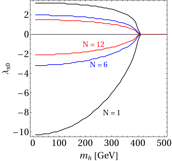
For a given $\Lambda$ we shall require that there is no pole in the evolution of scalar quartic coupling constants at energies below $\Lambda$. The region in the $(\Lambda,m_{h}=v\sqrt{2\lambda_{H\,0}})$ plane allowed by this constraint, depends on the initial parameters $\lambda_{x\,0}$, $\lambda_{\varphi\,0}$, and the number of scalars $N$. For each $\Lambda$ the maximum allowed value of $m_{h}$ constitutes the triviality bound on the Higgs mass. One might worry that each quartic coupling constant will have a different pole location, this, however, does not occur when $\lambda_{x\,0}\neq 0$ (as we assume), for then all the RGE equations are coupled and $\lambda_{H,\varphi,x}$ diverge at the same value of $\mu$.

The triviality bound for $m_{h}$ as a function of $\Lambda$ is illustrated in Fig. 1. Note that the allowed region shrinks as $\lambda_{x\,0}$ grows for fixed $N$, and as $N$ increases for fixed $\lambda_{x\,0}$, lowering the upper bound on $m_{h}$ in either case. This behavior is a direct consequence of the term $2N\lambda_{x}^{2}$ in (4.1): increasing $N$ and/or $\lambda_{x}$ amplifies the evolution of $\lambda_{H}$. For a given $(\Lambda,m_{h})$ and fixed $\lambda_{\varphi\,0}$ there is a range of $\lambda_{x\,0}$ for which the Landau pole occurs above $\Lambda$, as shown in Fig. 3. Note the asymmetry of the allowed (inner) region, which is a consequence of the $8\lambda_{x}^{2}$ term in (4.2).

In Fig.2 we show triviality limits for $\lambda_{\varphi}$ as a function of $\Lambda$ for the case $\lambda_{x\,0}=0$ when the $\vec{\varphi}$ evolution decouples from the SM.

If we assume that the SM is an effective theory valid at scales below the UV cutoff $\Lambda$, radiative corrections  [22] shift the Higgs mass to a scale of order $\Lambda/\sqrt{4\pi}$. The existing bounds on the scale of new physics imply $\Lambda>O(\;\hbox{TeV})$, which is in conflict with a Higgs mass below $1$ TeV range as required by the unitarity constraint [20]. A way of alleviating this conflict is to arrange cancellations to occur within the $O(\Lambda^{2})$ contributions to $m_{h}^{2}$. These cancellations can be obtained through a fine tuning of the parameters or through a an extension of the SM together with an appropriate new symmetry (as is the case in supersymmetric models).

The first solution to this problem was proposed by Veltman  [22] who observed that the 1-loop quadratic corrections to $m_{h}$ would vanish if $m_{h}^{2}+m_{Z}^{2}+2m_{W}^{2}-4m_{t}^{2}=0$, but this possibility is now experimentally disallowed. Here we shall follow a similar approach within the multi-singlet extension of the SM.

In pursuing this approach it is important to determine the possible effects generated by higher order radiative corrections. In a theory with many couplings $\lambda_{i}$ the general form of leading higher-order contributions (those containing the highest power of $\log(\Lambda)$) to the quadratically divergent contributions to $m_{h}^{2}$ at $n+1$ loops take the form [23]

where $\mu$ is the renormalization scale and the coefficients $f_{n}$ satisfy

Thus in order to determine the two-loop leading logarithmic corrections to the Higgs mass one needs the one-loop corrections and the first order beta functions (for generic results and applications to the single scalar case see [24]). The results for $N$-singlet model read:

the logarithmic terms ($\propto m_{\varphi}^{2}\log\Lambda$) in the one-loop correction were kept since they are relevant in the range $m_{h}\ll m_{\varphi}\mathrel{\raise 1.29167pt\hbox{$<$\kern-7.5pt\lower 4.30554pt\hbox{$\sim$}}}\Lambda$); terms $\propto m_{h}^{2}\log\Lambda$ are always numerically negligible and are included for completeness. For the numerical results the renormalization scale was chosen to be the vacuum expectation value of the Higgs field, $\mu=246\;\hbox{GeV}$. The SM result can be recovered in the limit $\lambda_{x}=\lambda_{\varphi}=0$.

We implement the fine tuning condition in a standard manner [18] by requiring

and determine the region in the $(\Lambda,m_{h})$ plane where this is obeyed for a given choice of the fine tuning parameter $\Delta_{h}$. Specifically, for each choice of $(\Lambda,m_{h})$ with fixed $N$ and $\lambda_{x}$ we check if there exist $m_{\varphi}$ and $\lambda_{\varphi}$ such that condition (5.5) is satisfied; the results are presented in Figs. 4 and 5.

It is worth noting that the two-loop $\vec{\varphi}$ corrections to $m_{h}$ (5.4) grow as $\lambda_{x}/(16\pi^{2})\ln(\Lambda/\mu)$ relative to the one-loop contributions(5.3). Perturbative consistency then requires this factor to be $\leq 1$, which translates into a maximal cutoff $\Lambda_{\rm max}$ beyond which perturbation theory is no valid:

Therefore the regions of large $\Lambda$ in Figs. 4 and 5 should be considered with a certain caution (that should increase with $\lambda_{x}$). The range of $\Lambda$ is extended up to $10^{6}\;\hbox{GeV}$ only for the purpose of the SM ($\lambda_{x}=0$) and small $\lambda_{x}$ cases ($\lambda_{x}\mathrel{\raise 1.29167pt\hbox{$<$\kern-7.5pt\lower 4.30554pt\hbox{$\sim$}}}0.95$ for $\mu=246\;\hbox{GeV}$).

We now consider the regions in the $(\Lambda,m_{h})$ excluded by the triviality and fine tuning constraints, first for $\lambda_{x}\geq 0$ and then for $\lambda_{x}<0$.

The singlet $\vec{\varphi}$, being odd under the $Z_{2}$ symmetry, is stable, and therefore a dark matter candidate, in which case the parameters of the theory should also lead to the DM abundance consistent with the WMAP observations, ${\Omega_{\mathrm{DM}}^{\mathrm{(exp)}}}=0.110\pm 0.018$ ($3\sigma$) [26]. In order to gauge the consequences of this constraint on our model we first calculate the relic DM abundance by solving the appropriate Boltzmann equation. Considering first the single component ($N=1$) case, we have [27]:

where $f\equiv n/T^{3}$, $n$ is the particle number density of the DM candidate (in our case the singlet), $f_{EQ}(T)$ is the equilibrium distribution, $g_{\star}(T)$ is the number of relativistic degrees of freedom at temperature $T$, $m_{Pl}$ is the Planck mass and $\left\langle\sigma v\right\rangle$ is the thermally-averaged cross section for $DM+DM\rightarrow SM+SM$ annihilation processes ([28], [10]):

where $x=m_{\varphi}/T$, $K_{1,2}(x)$ are the modified Bessel functions, and $\sigma(s)$ is the $DM+DM\rightarrow SM+SM$ annihilation cross section normalized in the standard manner. In analytical estimates is useful to note that $\left\langle\sigma v\right\rangle\sim\hat{\sigma}(4m_{\varphi}^{2})/4m_{\varphi}^{2}$ for non-relativistic DM; however we do not use this approximation in the numerical results shown below.

In the case of $N$-singlet scalar DM candidates with $O(N)$ symmetry, all components contribute equally to the relic abundance, just like a single field with $N$ degrees of freedom. Therefore the total abundance equals

where $\Omega_{\mathrm{DM}}^{i}$ is the dark matter relic density from the $i$-th scalar field. By virtue of the $O(N)$ symmetry it is sufficient to consider the Boltzmann equation for one of the components of $\vec{\varphi}$.

In the following we will discuss two different limiting cases for the Boltzmann equation: Cold Dark Matter (CDM) and Feebly Interacting Dark Matter (FIDM). We do not consider the hot dark matter solution, since it is inconsistent with structure formation at the galaxy scale, see e.g. [29].

The diagrams contributing to $\vec{\varphi}\vec{\varphi}$ annihilation into SM particles are shown in Fig. 6. The corresponding cross sections (for $N=1$) are available in the literature (e.g. [5] and [10]); we have verified the results of [10]:

where $F(\xi)=\mathrm{ArcTanh}(\xi)/\xi$, $\xi=\sqrt{(s-4m_{h}^{2})(s-4m_{\varphi}^{2})}/(s-2m_{h}^{2})$. The total cross section is then

where the sum runs over all fermions $f$.

When $N>1$ one has to modify the Higgs width as it can decay into $N$ possible $\varphi_{i}\varphi_{i}$ final states:

where $\theta_{H}$ is the Heaviside step function.

In this section we discuss constraints imposed on the model by searches for direct signals of DM particles scattering off nuclei. Even though the results of many experiments are available, here we will concentrate on the constraints obtained by the XENON100 experiment [32] as they impose strongest limits on DM - nucleon scattering cross-section $\sigma_{\rm DM-N}$ in the mass range of our interest; at the end of this section we also comment on the recent results for the CRESST-II experiment [19].

The relevant scattering amplitude is described by the Feynman diagram in Fig. 10; the corresponding cross section is

where the sum runs over all quark flavors $q$, $m_{n}$ is the nucleon mass and $f^{N}_{q}$ are the nucleon form factors as defined in [30].

In Fig. 11 we show the regions in the $(m_{\varphi},m_{h})$ plane allowed by the XENON100 limits [32] on $\sigma_{\rm DM-N}$. In the left panel the low $m_{\varphi}$ region is magnified to illustrate the two allowed bands. The one corresponding to the resonance region $m_{h}\sim 2m_{\varphi}$ (see also Fig. 7); for these values the annihilation is amplified to such an extent that (6.14) requires a very small coupling $\lambda_{x}$ so that this region is allowed by the direct detection. Since the XENON100 data is available for $m_{\varphi}\geq 5\;\hbox{GeV}$ therefore the vertical band of masses below $5\;\hbox{GeV}$ is also allowed. The right panel shows the large allowed area available for increasing $m_{DM}$ where the sensitivity of XENON100 is reduced.

Recently a positive result for a direct detection in elastic scattering of DM particles off nucleons was announced [19] by the CRESST-II collaboration; with two points selected by a maximum likelihood fit (Tab. 4 and Fig. 8 in [19]) $M1:\;\{m_{\rm DM}=25.3\;\hbox{GeV},~\sigma_{\rm DM-N}=11.6\cdot 10^{-6}\;\hbox{pb}\}$ and $M2:\;\{m_{\rm DM}=11.6\;\hbox{GeV},~\sigma_{\rm DM-N}=3.7\cdot 10^{-5}\;\hbox{pb}\}$. These cross sections are far above lower limit from XENON100 experiment [32], an issue that is yet to be resolved. As a complement to the implications derived above using the XENON100 limits, we will also discuss the consequences the CRESST-II results would have in constraining our model.

For each choice of $m_{h}$ and $N$ the requirement (6.14) determines a narrow allowed band in the $(\lambda_{x},m_{\varphi})$ plane; an example is provided in Fig. 7 for the CDM case with $m_{h}=130\;\hbox{GeV}$ and $N=1,6,12$. It is natural to ask weather there exist $m_{h}$ (in the region allowed by the present data) and $N$ such that the corresponding band contains the most likely points $M1$ and $M2$ found by CRESST-II. The answer is contained in the top panels of Fig. 12, where the regions preferred by CRESST-II (within $2\sigma$) are superimposed with predictions of our model for $N=1,~2$ and $m_{h}=110-140\;\hbox{GeV}$ when satisfying (6.14) at the $3\sigma$ level. As it is seen from the figure both regions are consistent with the model. For larger values of $N$ our model is consistent only with the 2$\sigma$ $M1$ contour for $m_{\varphi}\sim 50\;\hbox{GeV}$. If confirmed, these data would provide a strong restriction on the scenario discussed in this paper; in particular a tightening of the allowed regions around the current central values would require $N\mathrel{\raise 1.29167pt\hbox{$<$\kern-7.5pt\lower 4.30554pt\hbox{$\sim$}}}5$. Moreover it has immediate and dramatic consequences for Higgs boson searches at Tevatron or LHC since the invisible $h\to\vec{\varphi}\vec{\varphi}$ decay has a substantial branching ratio for the parameter regions consistent with $M1$ or $M2$. This is illustrated in the middle and bottom panels of Fig. 12, where the branching ratio is plotted against scalar mass $m_{\varphi}$.

When $\lambda_{x}<0$, the constraint (3.3) generates no restrictions and the branching ratio can be very large, $BR_{h\to\vec{\varphi}\vec{\varphi}}\sim 1$ (see middle panels of Figs. 12 and 13). In these figures we also plot maximum value of $BR_{h\to\vec{\varphi}\vec{\varphi}}$ calculated for $|\lambda_{x}|$ that saturates the vacuum stability bound (3.1) on $|\lambda_{x}|$ for a given quartic $\vec{\varphi}$ self coupling $\lambda_{\varphi}=8\pi,1,0.5$ and $0.1$, when $m_{h}=130\;\hbox{GeV}$; the regions above corresponding dashed curves are excluded by this constraint.

For $\lambda_{x}>0$ the constraint (3.3) is important and excludes the region above the dotted curve shown in the bottom panels of Fig. 12 and 13. Within the allowed region the $BR_{h\to\vec{\varphi}\vec{\varphi}}$ is smaller, but it can still reach $\sim 0.8$.

Note, that if one anticipates the cutoff $\Lambda$ to be below $\sim 10^{4}\;\hbox{GeV}$ (as we do in this work) then the triviality upper limit for low $N$ is roughly $\lambda_{\varphi}\mathrel{\raise 1.29167pt\hbox{$<$\kern-7.5pt\lower 4.30554pt\hbox{$\sim$}}}5$, so the branching ratio could easily reach even $99\%$ without any conflict with triviality. It is also worth mentioning here that if $\lambda_{x}>0$, then small value of $m_{\varphi}$ in the $M1$ and $M2$ regions together with the consistency condition (3.3) imply $0.06<\lambda_{x}<0.24$, which is too small to ameliorate the SM fine tuning problem (see Sec. 5). On the other hand, if $\lambda_{x}<0$, the vacuum stability bound (3.1) implies $|\lambda_{x}|<0.85$ for $\lambda_{\varphi}\leq 8\pi$ and $110\;\hbox{GeV}<m_{h}<141\;\hbox{GeV}$; then, as seen from Fig. 5, the allowed values for the cutoff $\Lambda$ are smaller than for the SM. Therefore $\lambda_{x}<0$ does not help solving the hierarchy problem regardless of the cosmological constraints.

From the top panels of Figs. 12 and 13 one observes that for $1\leq N\leq 12$ low Higgs boson masses ($m_{h}=110-120\;\hbox{GeV}$) are preferred by the $M1$ region of heavier $\vec{\varphi}$ (larger $N$ favors smaller $m_{h}$). For the region of lighter $m_{\varphi}$ ($M2$) roughly all Higgs boson masses fit data equally well, however only for $N=1$ and 2.

In conclusion, the CRESST-II positive result, if confirmed, would imply (within the singlet extension of the SM) that the Higgs boson could decay mainly invisibly, escaping discovery at both Tevatron and LHC. The option of invisibly decaying Higgs boson have been considered previously in [33].

In spite of its many successes, the standard CDM cosmological model is also facing some difficulties when compared with recent observations. For instance, high-resolution N-body simulations have shown that the model generates a cusps in the DM density distribution in central regions of galaxies [34]. Another discrepancy concerns the number of subhalos predicted by the model, which is at least factor of ten larger than the observed [35] number. Self-interacting DM was proposed by Spergel & Steinhardt [36] to cure these problems. Within this model, dark matter particles experience weak, non-dissipative collisions on scales of kpc to Mpc for typical galactic densities. This effect then generates a soft core in the inner regions of the dark halos, and it also ameliorates the overabundance of subhalos. The key requirement is that the mean free path of DM particles should be between 1 kpc and 1 Mpc in regions where the dark matter density is about $0.4\;\hbox{GeV}/{\rm cm}^{3}$. This model has attracted much attention [37].

In order to discuss this idea quantitatively we define the elastic scattering cross section per unit mass for DM consisting of $N$ species. We then imagine a clump of DM particles scattering off another such clump: