Low-rank optimization with trace norm penaltyThanks: This paper presents research results of the Belgian Network DYSCO (Dynamical Systems, Control, and Optimization), funded by the Interuniversity Attraction Poles Programme, initiated by the Belgian State, Science Policy Office. The scientific responsibility rests with its authors.
Abstract
The paper addresses the problem of low-rank trace norm minimization. We propose an algorithm that alternates between fixed-rank optimization and rank-one updates. The fixed-rank optimization is characterized by an efficient factorization that makes the trace norm differentiable in the search space and the computation of duality gap numerically tractable. The search space is nonlinear but is equipped with a particular Riemannian structure that leads to efficient computations. We present a second-order trust-region algorithm with a guaranteed quadratic rate of convergence. Overall, the proposed optimization scheme converges super-linearly to the global solution while maintaining complexity that is linear in the number of rows and columns of the matrix. To compute a set of solutions efficiently for a grid of regularization parameters we propose a predictor-corrector approach that outperforms the naive warm-restart approach on the fixed-rank quotient manifold. The performance of the proposed algorithm is illustrated on problems of low-rank matrix completion and multivariate linear regression.
1 Introduction
The present paper focuses on the convex program
| (1) |
where is a smooth convex function, is the trace norm (also known as nuclear norm) which is the sum of the singular values of [Faz02, RFP10, CCS10] and is the regularization parameter. Programs of this type have attracted much attention in the recent years as efficient convex relaxations of intractable rank minimization problems [Faz02]. The rank of the optimal solution of (1) decreases to zero as the regularization parameter grows unbounded [Bac08]. As a consequence, generating efficiently the regularization path , for a whole range of values of minimizers, is a convenient proxy to obtain suboptimal low-rank minimizers of .
Motivated by machine learning and statistical large-scale regression problems [RFP10, YELM07, VNMA10], we are interested in very low-rank solutions () of very high-dimensional problems (). To this end, we propose an algorithm that guarantees second-order convergence to the solutions of (1) while ensuring a tight control (linear in ) on the data storage requirements and on the numerical complexity of each iteration.
The proposed algorithm is based on a low-rank factorization of the unknown matrix, similar to the singular value decomposition (SVD), . Like in SVD, and are orthonormal matrices that span row and column spaces of . In contrast, the scaling factor is allowed to be non-diagonal which makes the factorization non-unique.
Our algorithm alternates between fixed-rank optimization and rank-one updates. When the rank is fixed, the problem is no longer convex but the search space has nevertheless a Riemannian structure. We use the framework of manifold optimization to devise a trust-region algorithm that generates low-cost (linear in ) iterates that converge super-linearly to a local minimum. Local minima are escaped by incrementing the rank until the global minimum in reached. The rank-one update is always selected to ensure a decrease of the cost.
Implementing the complete algorithm for a fixed value of the regularization parameter leads to a monotone convergence to the global minimum through a sequence of local minima of increasing ranks. Instead, we also modify along the way with a predictor-corrector method thereby transforming most local minima of (1) (for fixed and fixed rank) into global minima of (1) for different values of . The resulting procedure, thus, provides a full regularization path at a very efficient numerical cost.
Not surprisingly, the proposed approach has links with several earlier contributions in the literature. Primarily, the idea of interlacing fixed-rank optimization with rank-one updates has been used in semidefinite programming [BM03, JBAS10]. It is here extended to a non-symmetric framework using the Riemannian geometry recently developed in [BS09, Mey11, MBS11]. An improvement with respect to the earlier work [BM03, JBAS10] is the use of duality gap certificate to discriminate between local and global minima and its efficient computation thanks to the chosen parameterization.
Schemes that combine fixed-rank optimization and special rank-one updates have appeared recently in the particular context of matrix completion [KO09, WYZ12]. The framework presented here is in the same spirit but in a more general setting and with a global convergence analysis. Most other fixed-rank algorithms [SJ03, KO09, MJD09, SE10, WYZ12, Mey11, BA11, Van13] for matrix completion are first-order schemes. It is more difficult to provide a tight comparison of the proposed algorithm to trace norm minimization algorithms that do not fix the rank a priori [CCS10, MHT10, YELM07, AFSU07]. It should be emphasized, however, that most trace norm minimization algorithms use singular value thresholding operation at each iteration. This is the most numerically demanding step for these algorithms. For the matrix completion application, it involves computing (potentially all) the singular values of a low-rank + sparse matrix [CCS10]. In contrast, the proposed approach requires only dense linear algebra (linear in ) and rank-one updates using only dominant singular vectors and value of a sparse matrix. The main potential of the algorithm appears when computing the solution not for a single parameter but for a number of values of . We compute the entire regularization path with an efficient predictor-corrector strategy that convincingly outperforms the warm-restart strategy.
For the sake of illustration and empirical comparison with state-of-the-art algorithms we consider two particular applications, low-rank matrix completion [CR09] and multivariate linear regression [YELM07]. In both cases, we obtain iterative algorithms with a numerical complexity that is linear in the number of observations and with favorable convergence and precision properties.
2 Relationship between convex program and non-convex formulation
Among the different factorizations that exist to represent low-rank matrices, we use the factorization [MBS11, BS09] that decomposes a rank- matrix into
where , and . is the Stiefel manifold or the set of matrices with orthonormal columns. is the cone of positive definite matrices. We stress that the scaling is not required to be diagonal. The redundancy of this parameterization has non-trivial algorithmic implications (see Section 3) but we believe that it is key to success of the approach. See [KO09, MBS11] for earlier algorithms advocating matrix scaling and Section 6.1 for a numerical illustration. With the use of factorization , the trace norm is written as which makes it differentiable. For a fixed rank , the optimization problem (1) is recast as
| (2) |
The search space of (2) is not Euclidean but the product space of two well-studied manifolds, namely, the Stiefel manifold [EAS98] and the cone of positive definite matrices [Smi05]. This provides a proper geometric framework to perform optimization. From the geometric point of view, the column and row spaces of are represented on the Stiefel manifold whereas the scaling factor is absorbed into the positive definite part. A proper metric on the space takes into account both rotational and scaling invariance.
2.1 First-order optimality conditions
In order to relate the fixed-rank problem (2) to the convex optimization problem (1) we look at the necessary and sufficient optimality conditions that govern the solutions. The first-order necessary and sufficient optimality condition for the convex program (1) is
| (3) |
where is the Euclidean gradient of in at and is the sub-differential of the trace norm (optimality conditions for trace norm are in [Bac08, RFP10]).
Proposition 2.1.
The first-order necessary optimality conditions of (2)
| (4) |
where , for any square matrix and . is referred to as dual variable throughout the paper.
Proof.
Proposition 2.2.
Proof.
2.2 Duality gap computation
Proposition 2.2 provides a criterion to check the global optimality of a solution of (2). Here however, it provides no guarantees on closeness to the global solution. A better way of certifying closeness for the optimization problem of type (1) is provided by the duality gap. The duality gap characterizes the difference of the obtained solution from the optimal solution and is always non-negative [BV04].
Proposition 2.3.
Proof.
The proof is given in Appendix A.4. ∎
When , the expression of duality gap is
| (6) |
where is the dual candidate. A good choice for the dual candidate is with appropriate scaling to satisfy the operator norm constraint: [BJMO11]. As an extension for some functions of type where is a linear operator, computing the Fenchel conjugate of the function may be easier than that of . When the duality gap, using similar calculations as above, is where is the adjoint operator of and is the Fenchel conjugate of . A good choice of is again where is the dominant singular value of [BJMO11].
3 Manifold-based optimization to solve the non-convex problem (2)
In this section we propose an algorithm to obtain a local minimum for the problem (2). In contrast to first-order optimization algorithms proposed earlier in [MBS11, MBS10, KO09], we develop a second-order trust-region algorithm that has a quadratic rate of convergence [NW06, AMS08]. The idea behind a trust-region algorithm is to build locally a quadratic model of the function at a point and solve the trust-region subproblem to get the next potential iterate. Depending on whether the decrease in the objective function is sufficient or not, the potential iterate is accepted or rejected. Details about a general trust-region algorithm are given in [NW06]. We rewrite (2) as
| (7) |
where is introduced for notational convenience. An important observation for second-order algorithms [AIDLVH09, AMS08] is that the local minima of the problem (7) are not isolated in the search space
This is because the cost function is invariant under rotations, for any rotation matrix . Note that takes away all the symmetry of the total space. This is done by counting the dimension of the quotient space11 1 The dimension of the total space is and that of is . Hence, the dimension of the quotient space is equal to dimension of total space dimension of . which is . This is same as dimension of the rank- matrices.
To remove the symmetry of the cost function, we identify all the points of the search space that belong to the equivalence class defined by
The set of all such equivalence classes is denoted by
| (8) |
which has the structure of a smooth quotient manifold by [Lee03, Theorem ]. Problem (7) is thus conceptually an unconstrained optimization problem on the quotient manifold in which the minima are isolated. Computations are performed in the total space , which is the product space of well-studied manifolds.

Tangent space of
Tangent vectors at a point have a matrix representation in the tangent space of the total space . Note that belongs to and its equivalence class is represented by the element such that . Because the total space is a product space , its tangent space admits the decomposition at a point
and the following characterizations are well-known [EAS98, Smi05]
where is the set of symmetric matrices.
Note that an arbitrary matrix is projected on the tangent space by the linear operation
| (9) |
where . A matrix representation of the tangent space at relies on the decomposition of into its vertical and horizontal subspaces. The vertical space is the subspace of that is tangent to the equivalence class
| (10) |
where is the set of skew symmetric matrices of size . The horizontal space must be chosen such that . We choose as the orthogonal complement of for the metric
| (11) |
which picks the normal metric of the Stiefel manifold [EAS98] and the natural metric of the positive definite cone [Smi05]. Here and are elements of . With this choice, a horizontal tangent vector is any tangent vector belonging to the set
| (12) |
for all . Another characterization of the horizontal space is . The horizontal space is invariant by the group action along the equivalence class. Starting from an arbitrary tangent vector we construct its projection on the horizontal space by picking such that
| (13) |
Using the calculation (12), the unique that satisfies (13) is the solution of the Lyapunov equation
| (14) |
where and is the matrix representation of . The numerical complexity of solving the Lyapunov equation is [BS72].
The Riemannian submersion
The choice of the metric (11), which is invariant along the equivalence class turns the quotient manifold into a Riemannian submersion of [Lee03, Theorem ] and [AMS08, Section ]. As shown in [AMS08], this special construction allows for a convenient matrix representation of the gradient [AMS08, Section ] and the Hessian [AMS08, Proposition ] on the abstract manifold . The Riemannian gradient of is uniquely represented by its horizontal lift in which has the matrix representation
| (15) |
It should be emphasized that is in the the tangent space . However, due to invariance of the cost function along the equivalence class , also belongs to the horizontal space and hence, the equality in (15) [AMS08]. The matrix expression of in the total space at a point is obtained from its definition: it is unique element of that satisfies for all . is the standard Euclidean directional derivative of in the direction . This definition leads to the matrix representations
| (16) |
where is and is the gradient of in the Euclidean space . Here is projection operator (9).
Likewise, the Riemannian connection on is uniquely represented by its horizontal lift in which is where and are vector fields in and and are their horizontal lifts in . Once again, the Riemannian connection on has well-known expression [Jou09, Smi05, AMS08], obtained by means of the Koszul formula. The Riemannian connection on the Stiefel manifold is derived in [Jou09, Example ] and on the positive definite cone is derived in [Mey11, Appendix B]. Finally, the Riemannian connection on the total space is given by
| (17) |
Here is the classical Euclidean directional derivative of in the direction . The Riemannian Hessian in has, thus, the following matrix expression
| (18) |
for any and its horizontal lift .
Trust-region subproblem and retraction on
Trust-region algorithms on a quotient manifold with guaranteed quadratic rate convergence have been proposed in [AMS08, Algorithm ]. The convergence of the trust-region algorithm is quadratic because the assumptions [AMS08, Theorem ] are satisfied locally. The trust-region subproblem on is formulated as
where is the trust-region radius and and are the Riemannian gradient and Hessian on . The problem is horizontally lifted to the horizontal space where it is solved using a truncated-conjugate gradient method with parameters set as in [ABG07, Alg 2]. Solving the above trust-region subproblem leads to a direction that minimizes the quadratic model.
To find the new iterate based on the obtained direction , a mapping in the tangent space to the manifold is required. This mapping is more generally referred to as retraction which maps the vectors from the tangent space onto the points on the manifold, (details in [AMS08, Definition 4.1.1]). In the present case, a retraction of interest is [AMS08, MBS11]
| (19) |
where is a function that extracts the orthogonal factor of the polar factorization, i.e., and is the matrix exponential operator. The retraction on the positive definite cone is the natural exponential mapping for the metric (11) [Smi05]. These well-known retractions on the individual manifolds is also a valid retraction on the quotient space by virtue of [AMS08, Proposition ].
Numerical complexity
The numerical complexity per iteration of the proposed trust-region algorithm to solve (7) depends on the computational cost of the following components.
- •
Objective function problem dependent
- •
Metric
- •
Euclidean gradient of problem dependent
- •
- –
problem dependent
- –
Matrix
- –
Matrix
- –
Matrix
- –
- •
Projection operator
- •
Projection operator
- –
Lyapunov equation for
- –
- •
Retraction
As shown above all the manifold related operations have linear complexity in and . Other operations depend on the problem at hand and are computed in the search space . With the computational burden on the algorithm considerably reduces.
4 An optimization scheme to solve convex program (1)
Starting with rank problem, we alternate a second-order local optimization algorithm on fixed-rank manifold with a first-order rank-one update. The scheme is shown in Table 1. The rank update ensures that the cost is decreased and the new point belongs to .
Proposition 4.1.
If is a stationary point of (2) then the rank-one update
| (20) |
ensures a decrease in the objective function provided that is sufficiently small and the descent directions and are the dominant left and right singular vectors with singular value of the dual variable . The maximum decrease in the objective function is obtained for where is the Lipschitz constant such that for all .
Proof.
Algorithm to solve convex problem (1) 0. • Initialize to , a guess rank. • Initialize the threshold for convergence criterion, refer to Proposition 2.2. • Initialize the iterates , and . 1. Solve the non-convex problem (2) in the dimension to obtain a local minimum . 2. Compute (the dominant singular value) of dual variable . • If (or duality gap ) due to Proposition 2.2, output as the solution to problem (1) and stop. • Else, compute the update as shown in Proposition 4.1 and compute the new point as described in (21). Set and repeat step .
A representation of on is obtained from the singular value decomposition of . Since is a rank-one update of , the singular value decomposition can be performed efficiently [Bra06]. Defining and such that and , which are the orthogonal projections of and on the complementary space of and , the update (20) is written as
where
It should be noted that is of size . If is the singular value decomposition of where and are orthonormal matrices and is a diagonal matrix then the new iterate is
| (21) |
To compute an Armijo-optimal we perform a backtracking line search starting from the value where is the Lipschitz constant for the gradient of [Nes03]. The justification for this value is given in Appendix A.3. In many problem instances a good value of can be well-approximated.
There is no theoretical guarantee that the algorithm in Table 1 stops at where is the optimal rank. However, convergence to the global solution is guaranteed from the fact that the algorithm alternates between fixed-rank optimization and rank updates (unconstrained projected rank-1 gradient step) and both are descent iterates. Disregarding the fixed-rank step, the algorithm reduces to a gradient algorithm for a convex problem with classical global convergence guarantees. This theoretical certificate however does not capture the convergence properties of an algorithm that empirically always converges at a rank (most often at the optimal rank) One advantage of the scheme, in contrast to trace norm minimization algorithms proposed in [CCS10, TY10, MGC11, MHT10], is that it offers a tighter control of the rank at all intermediate iterates of the scheme. It should be also be emphasized that the stopping criterion threshold of the non-convex problem (2) and of the convex problem (1) are chosen separately. This means that rank-increments can be made after a fixed number of iterations of the manifold optimization without waiting for the trust-region algorithm to converge to a local minimum.
5 Regularization path
In most applications, the optimal value of is unknown [MHT10] and which means that in fact problem (1) be solved for a number of regularization parameters. In addition, even if the optimal is a priori known, a path of solutions corresponding to different values of proves interpretability to the intermediate iterates which are now global minima for different values of . This motivates to compute the complete regularization path of (1) for a number of values , i.e., defined as where is the solution to the minimization problem.
A common approach is the warm-restart approach where the algorithm to solve the problem is initialized from and so on [MHT10]. However, the warm-restart approach does not use the fact that the regularization path is smooth especially when the values of are close to each other. An argument towards this is given later in the paragraph. In this section we describe a predictor-corrector scheme that takes into account the first-order smoothness and computes the path efficiently. To compute the path we take a predictor (estimator) step to predict the solution and then rectify the prediction by a corrector step. This scheme has been widely used in solving differential equations and regression problems [PH06]. We extend the prediction idea to the quotient manifold . The corrector step is carried out by initializing the algorithm in Table 1 from the predicted point. If is the fixed-rank factorization then the solution of the optimization problem is predicted (or estimated), i.e., , by the two previous solutions and at and respectively belonging to the same rank manifold . When and belong to different rank manifolds we perform instead a warm restart to solve problem. The complete scheme is shown in Table 2 and has the following advantages.
- •
With a few number of rank increments we traverse the entire path.
- •
Potentially every iterate of the optimization scheme is now a global solution for a value of .
- •
The predictor-corrector approach outperforms the warm-restart approach in maximizing prediction accuracy with minimal extra computations.
In this section, we assume that the optimization problem (1) has a unique solution for all . A sufficient condition is that is strictly convex, which can be enforced by adding a small multiple of the square Frobenius norm to . The global solution is uniquely characterized by the non-linear system of equations
which is obtained from the optimality conditions (4) and Proposition 2.2. The smoothness of with respect to follows from the Implicit Function Theorem [KP02]. Another reasoning is by looking at the geometry of the dual formulation. Note that we employ the predictor-corrector step only when we are on the fixed-rank manifold which corresponds to a face of the dual operator norm set. From (5), the dual optimal solution is obtained by projection onto the dual set Smoothness of the dual variable with respect to follows from the smoothness of the projection operator [HUL93]. Consequently, smoothness of the primal variable follows from the smoothness assumption of .
Computing the regularization path 0. Given in decreasing order. Also given are the solutions and at and respectively and their low-rank factorizations. 1. Predictor step: • If and belong to the same quotient manifold then construct a first-order approximation of the solution path at and estimate as shown in (23). • Else . 2. Corrector step: Using the estimated solution of the , initialize the algorithm described in Table 1 to compute the exact solution . 3. Repeat steps and for all subsequent values of .
Predictor step on the quotient manifold

Assuming (first-order) smoothness of the regularization path on connecting and in , we build a first-order approximation of the geodesic, i.e. the curve of shortest length, connecting the two points. The estimated solution is then computed by extending the first-order approximation of the geodesic. In other words, we need to identify a vector and its horizontal lift at on defined as that maps on to the horizontal space [AMS08]. is referred to as logarithmic mapping. Computing the logarithmic mapping (and hence, the geodesic) might be numerically costly in general. For the case of interest there is no analytic expression for the logarithmic mapping. Instead a numerically efficient way is to use the approximate inverse retraction where to obtain a direction in the space followed by projection onto the horizontal space . Note that . The projection is accomplished using projection operators and defined in Section 3. Hence, an estimate on is given as
| (22) |
For the retraction of interest (19) the Frobenius norm error in the approximation of the Logarithmic mapping is bounded as
The approximation error comes from the fact that the retraction used is at least a first-order retraction [AMS08]. This approximation is exact if is the Euclidean space. The approximate inverse retraction corresponding to the retraction described in (19) is computed as
where is the matrix logarithm operator. The predicted solution is then obtained by taking a step and performing a backtracking line search in the direction i.e.,
| (23) |
A good choice of the initial step size is . The motivation for the choice comes the observation that it is optimal when the solution path is a straight line in the Euclidean space. The numerical complexity to perform the prediction step in the manifold is .
6 Numerical Experiments
The overall optimization scheme with descent-restart and trust-region algorithm is denoted as “Descent-restart + TR” (TR). We test the proposed optimization framework on the problems of low-rank matrix completion and multivariate linear regression where trace norm penalization has shown efficient recovery. Full regularization paths are constructed with optimality certificates. All simulations in this section are performed in MATLAB on a GHz Intel Core machine with GB of RAM.
6.1 Diagonal versus matrix scaling
Before entering a detailed numerical experiment we illustrate here the empirical evidence that constraining to be diagonal (as is the case with SVD) is detrimental to optimization. To this end, we consider the simplest implementation of a gradient descent algorithm for matrix completion problem (see below). The plots shown Figure 3 compare the behavior of the same algorithm in the search space and (SVD). is the set of diagonal matrices with positive entries. The empirical observation that convergence suffers from imposing diagonalization on is a generic observation that does not depend on the particular problem at hand. The problem here involves completing a of rank from of observed entries. is fixed at .

6.2 Low-rank matrix completion
The problem of matrix completion involves completing an matrix when only a few entries of the matrix entries are known. Presented in this way the problem is “ill-posed” but becomes considerably interesting when in addition a low-rank reconstruction is also sought. Given an incomplete low-rank (but unknown) real matrix , a convex relaxation of the matrix completion problem is
| (24) |
for and a regularization parameter . Here denotes the Frobenius norm, matrix is an weight matrix with binary entries and the operator denotes element-wise multiplication. If is the set of known entries in then, if and otherwise. The problem of matrix completion is known to be combinatorially hard. However, by solving the convex relaxation (24) a low-rank reconstruction is possible with a very high probability [CR09, KO09] under certain assumptions on the number of observed entries. For an exact reconstruction, the lower bound on the number of known entries is typically of the order where is the rank of the optimal solution, . Consequently, it leads to a very sparse weight matrix , which plays a very crucial role for efficient algorithmic implementations. For our case, we assume that the lower bound on the number of entries is met and we seek a solution to the optimization problem (24). Customizing the terminology for the present problem, the convex function is . Using the factorization , the rank- objective function is where . The dual variable .
The matrix representation of the gradient of in is , and . The Euclidean directional derivative of the gradient of along is where is the directional derivative of along . The Riemannian gradient and Hessian are computed using formulae developed in (16) and (18). Note that since is sparse, and are sparse too. As a consequence, the numerical complexity per iteration for the trust-region algorithm is of order where is the number of known entries. In addition computation of dominant singular value and vectors is performed with numerical complexity of [Lar]. The overall linear complexity with respect to the number of known entries allows us to handle potentially very large datasets.
Fenchel dual and duality gap for matrix completion
For the matrix completion problem, the sampling operation is the linear operator . We can, therefore, define a new function such that . The domain of is the non-zero support of . The dual candidate is defined by where and is the dominant singular value of (refer Section 2.2 for details). In matrix form, is written as . Finally, the Fenchel dual at a dual candidate can be computed is . The final expression for the duality gap at a point and a dual candidate is .
Next we provide some benchmark simulations for the low-rank matrix completion problem. For each example, a random matrix of rank is generated according to a Gaussian distribution with zero mean and unit standard deviation and a fraction of the entries are randomly removed with uniform probability. The dimensions of matrices of rank is . The over-sampling (OS) ratio determines the number of entries that are known. A over-sampling ratio of means that number of randomly and uniformly selected entries are known a priori out of entries.
6.2.1 An example
A random matrix of rank is generated as mentioned above. () of the entries are randomly removed with uniform probability. To reconstruct the original matrix we run the optimization scheme proposed in the Table 1 along with the trust-region algorithm to solve the non-convex problem. For illustration purposes is fixed at . We also assume that we do not have any a priori knowledge of the optimal rank and, thus, start from rank . The trust-region algorithm stops when the relative or absolute variation of the cost function falls below . The rank-incrementing strategy stops when relative duality gap is less than , i.e., . Convergence plots of the scheme are shown in Figure 4.


| Rel. error of reconstruction | |
|---|---|
| Recovered rank | |
| Duality gap | |
| Iterations |
A good way to characterize matrix reconstruction at is to look at the relative error of reconstruction, defined as,
Next, to understand low-rank matrix reconstruction by trace norm minimization we repeat the experiment for a number of values of all initialized from the same starting point and report the relative reconstruction error in Table 3 averaged over runs. This, indeed, confirms that matrix reconstruction is possible by solving the trace norm minimization problem (24).
| Rel. reconstruction error | ||||
|---|---|---|---|---|
| Recovered rank | ||||
| Iterations | ||||
| Time in seconds |
6.2.2 Regularization path for matrix completion
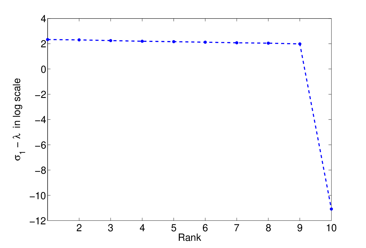
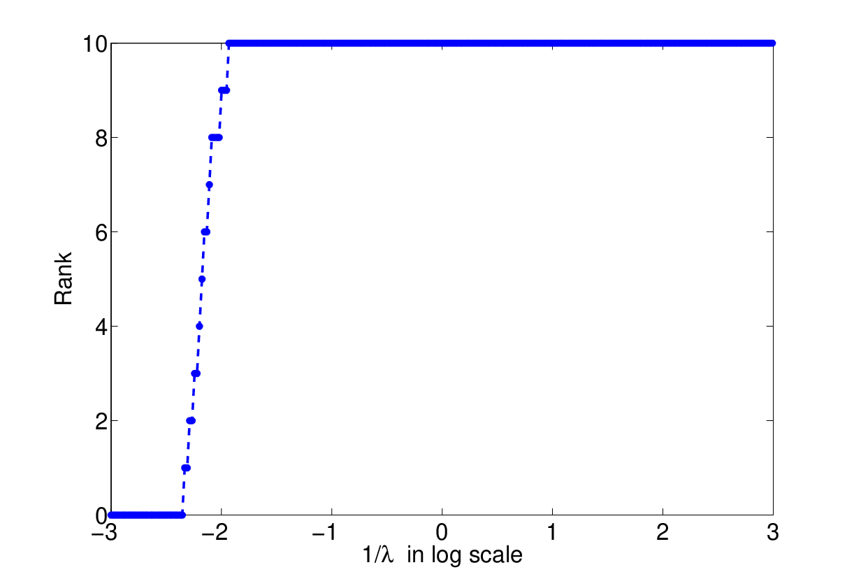
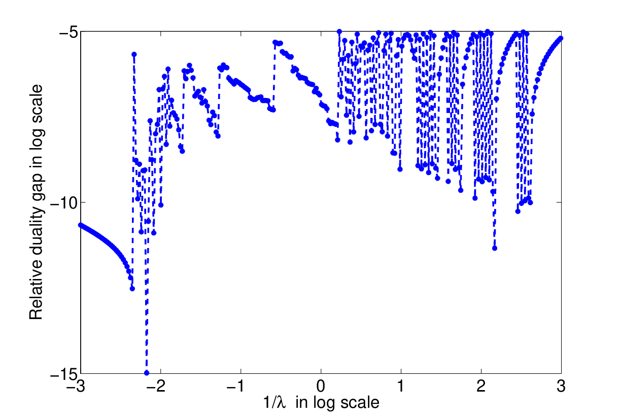
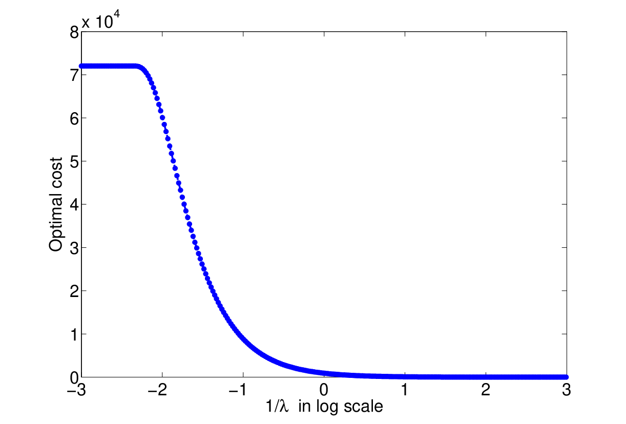
In order to compute the entire regularization path, we employ the predictor-corrector approach described in Table 2 to find solutions for a grid of values. For the purpose of illustration, a geometric sequence of values is created with the maximum value fixed at , the minimum value is set at and a reduction factor such that . We consider the same example as in Section 6.2.1. The algorithm for a stops when the relative duality gap falls below . Various plots are shown in Figure 5. Figure 5 also demonstrates the advantage of the scheme in Table 2 with respect to a warm-restart approach. We compare both approaches on the basis of
| (25) |
where is the global minimum at and is the prediction. A lower inaccuracy means better prediction.

| # values | |
|---|---|
| # iterations | |
| Time | seconds |
It should be emphasized that in Figure 4 most of the points on the curve of the objective function have no other utility than being intermediate iterates towards the global solution of the algorithm. In contrast all the points of the curve of optimal cost values in Figure 5 are now global minima for different values of .
6.2.3 Competing methods for matrix completion
In this section, we analyze the following state-of-the-art algorithms for low-rank matrix completion, namely,
- 1.
SVT algorithm by Cai et al. [CCS10]
- 2.
FPCA algorithm by Ma et al. [MGC11]
- 3.
SOFT-IMPUTE (Soft-I) algorithm by Mazumder et al. [MHT10]
- 4.
APG and APGL algorithms by Toh et al. [TY10]
While FPCA, SOFT-IMPUTE and APGL solve (24), the iterates of SVT converge towards a solution of the optimization problem
where is a regularization parameter. For simulation studies we use the MATLAB codes supplied on the authors’ webpages for SVT, FPCA and APGL. Due to simplicity of the SOFT-IMPUTE algorithm we use our own MATLAB implementation. The numerically expensive step in all these algorithms is the computation of the singular value thresholding operation. To reduce the computational burden FPCA uses a linear time approximate singular value decomposition (SVD). Likewise, implementations of SVT, SOFT-IMPUTE and APGL exploit the low-rank + sparse structure of the iterates to optimize the thresholding operation [Lar].
The basic algorithm FPCA by Ma et al. [MGC11] is a fixed-point algorithm with a proven bound on the iterations for accuracy. To accelerate the convergence they use the technique of continuation that involves approximately solving a sequence of parameters leading to the target . The singular value thresholding burden step is carried out by a linear time approximate SVD. The basic algorithm APG of Toh et al. is a proximal method [Nes03] and gives a much stronger bound on the number of iterations for accuracy. To accelerate the scheme, the authors propose three additional heuristics: continuation, truncation (hard-thresholding of ranks by projecting onto fixed-rank matrices) and a line-search technique for estimating the Lipschitz constant. The accelerated version is called APGL. The basic algorithm SOFT-IMPUTE iteratively replaces the missing elements with those given by an approximate SVD thresholding at each iteration. Accelerated versions involve post processing like continuation and truncation. It should be emphasized that the performance of SOFT-IMPUTE greatly varies with the singular values computation at each iteration. For our simulations we compute dominant singular values at each iteration of SOFT-IMPUTE.
Convergence behavior with varying
In this section we analyze the algorithms FPCA, SOFT-IMPUTE and Descent-restart + TR in terms of their ability to solve (24) for a fixed value of . For this simulation, we use FPCA, SOFT-IMPUTE and APGL without any acceleration techniques like continuation and truncation. SVT is not used for this test since it optimizes a different cost function. We plot the objective function against the number of iterations for a number of values. A random matrix of rank is generated under standard assumptions with over-sampling ratio ( of entries are removed uniformly). The algorithms Descent-restart + TR, FPCA and SOFT-IMPUTE and APG are initialized from the same point. The algorithms are stopped when either the variation or relative variation of is less than . The maximum number of iterations is set to. The rank incrementing procedure of our algorithm is stopped when the relative duality gap falls below .

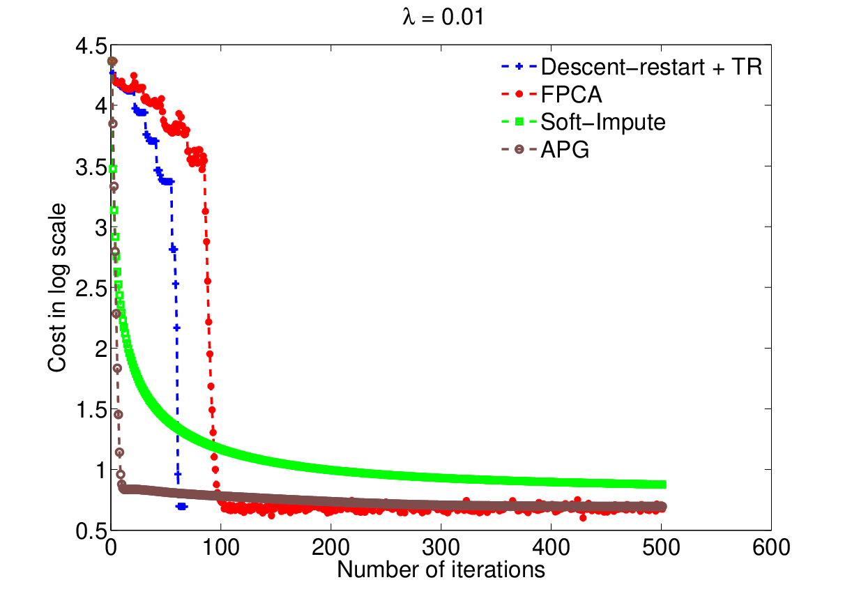
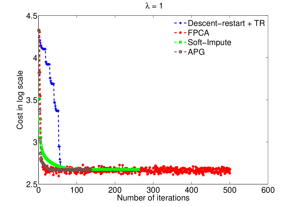
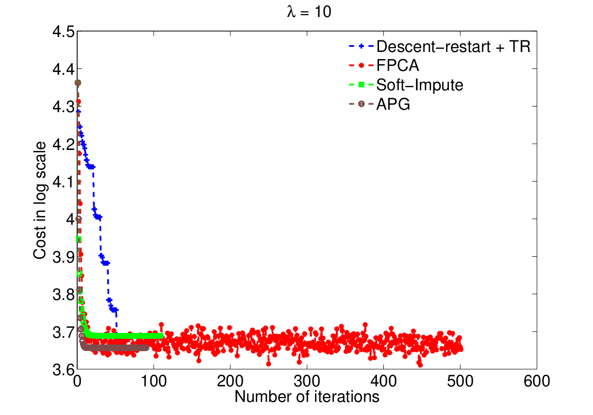
The plots are shown in Figure 6. The convergence behavior of FPCA is greatly affected by . It has a slow convergence for a small while for a larger , the algorithm fluctuates. SOFT-IMPUTE has a better convergence in all the three cases, however, the convergence suffers when a more accurate solution is sought. The performance of APG is robust to the change in values of . For moderate accuracy it outperforms all other algorithms. However, when a higher accuracy is sought it takes a large number of iterations. Descent-restart + TR, on the other hand, outperforms others in all the cases here with minimal number of iterations.
Convergence test
To understand the convergence behavior of different algorithms involving different optimization problems, we look at the evolution of the training error [CCS10, MHT10] defined as
| (26) |
with iterations. We generate a random matrix of rank under standard assumptions. The over-sampling ratio is kept at with slightly less of the entries being observed. The algorithms Descent-restart + TR, FPCA and SOFT-IMPUTE (Soft-I) are initialized from the same iterate with a fixed . We fix as it gives a good reconstruction to compare algorithms. For SVT we use the initialization including and a step size of as suggested in the paper [CCS10] where is the fraction of known entries. The algorithms are stopped when the variation or relative variation of Training error (26) is less than . The maximum number of iterations is set at . The rank incrementing procedure of our algorithm is stopped when the relative duality gap falls below .
APG has a fast convergence but the performance slows down later. Consequently, it exceeds the maximum limit of iterations. Similarly, SOFT-IMPUTE converges to a different solution but has a faster convergence in the initial phase (for iterations less than ). FPCA and Descent-restart + TR converge faster at a later stage of their iterations. Descent-restart + TR initially sweeps through ranks until arriving at the optimal rank where the convergence is accelerated owing to the trust-region algorithm.

Scaling test
To analyze the scalability of these algorithms to larger problems we perform a test where we vary the problem size from to . The reason for choosing a moderate value of is that large-scale implementations of SVT, FPCA and Soft-Impute are unavailable from authors’ webpages. For each , we generate a random matrix of size of rank under standard assumptions. Each entry is observed with uniform probability of [KO09]. The initializations are chosen as in the earlier example i.e., . We note the time and number of iterations taken by the algorithms until the stopping criterion is satisfied or when the number of iterations exceed . The stopping criterion is same as the one used before for comparison, when the absolute variation or relative variation of Training error (26) is less than . Results averaged over runs are shown in Figure 8. We have not shown the plots for SOFT-IMPUTE and APG as in all the cases either they did not converge in iterations or took much more time than the nearest competitor.


Below we have shown two more case studies where we intend to show the numerical scalability of our framework to a large scale instance. The first one involves comparisons with fixed-rank optimization algorithms. The second case is a large scale comparison with APGL (the accelerated version of APG). We consider the problem of completing a matrix of rank . The over-sampling ratio OS is implying that () of entries are randomly and uniformly revealed. The maximum number of iterations is fixed at .
Fixed-rank comparison
Because our algorithm uses a fixed-rank approach for the fixed-rank sub-problem, it is also meaningful to compare its performance with other fixed-rank optimization algorithms. However, a rigorous comparison with other algorithms is beyond the scope of the present paper. We refer to a recent paper [MMBS12] that deals with this question in a broader framework. Here we compare with two set-of-the-art algorithms that are LMaFit [WYZ12] and LRGeom (trust-region implementation) [Van13]. LMaFit is an alternating minimization scheme with a different factorization for a fixed-rank matrix. It is a tuned-version of the Gauss-Seidel non-linear scheme and has a superior time complexity per iteration. LRGeom is based on the embedded geometry of fixed-rank matrices. This viewpoint allows to simplify notions of moving on the search space. We use their trust-region implementation. The geometry leads to efficient guess of the optimal stepsize in a search direction. Plots in Figure 9 show a competitive performance of our trust-region scheme with respect to LMaFit. Asymptotically, both our trust-region scheme and LRGeom perform similarly but LRGeom performs much better in the initial few iterations.


Comparison with APGL
APG has a better iteration complexity than other class optimization algorithms. However, scalability of APG by itself to large dimensional problems is an issue. The principal bottleneck is that the ranks of the intermediate iterates seem to be uncontrolled and only asymptotically, a low-rank solution is expected. To circumvent this issue, an accelerated version of APG called APGL is also proposed in [TY10]. APGL is APG with three additional heuristics: continuation (a sequence of parameters leading to the target ), truncation (hard-thresholding of ranks by projecting onto fixed-rank matrices) and line-search technique for estimating the Lipschitz constant. We compare our algorithm with APGL. The algorithms are stopped when either absolute variation or relative variation of the objective function falls below . For our algorithm, the trust-region algorithm is also terminated with the same criterion. In addition, the rank-one update is stopped when the relative duality gap is below .
To solve (1) for a fixed APGL proceeds through a sequence of values for such that where is the iteration count of the algorithm. Initial is set to . We also follow a similar approach and create a sequence of values. A decreasing sequence is generated leading to is by using the recursive rule, when and otherwise until . Initial is set to . For we also relax the stopping criterion for the trust-region to as well as stopping the rank-one increment when relative duality gap is below as we are only interested for an accurate solution for .


We compete favorably with APGL in large scale problems for very low-ranks and when a higher accuracy is required. However, as the rank increases, APGL performs better. This is not surprising as our algorithm traverses all ranks, one by one before arriving at the optimal rank. In the process we spend a considerable effort in just traversing ranks. This approach is most effective only when computing in the full regularization path. Also for moderate accuracy, APGL performs extremely well. However, the better performance of APGL significantly relies on heuristics like continuation and truncation. The truncation heuristic allows the APGL algorithm to approximate an iterate by low and fixed-rank iterate. On the other hand, we strictly move in the low-rank space. This provides an efficient way to compute the full regularization path using a predictor-corrector strategy.
Comments on matrix completion algorithms
We summarize our observations in the following points.
- •
- •
- •
- •
APG has a better iteration complexity than the others and is well-suited when a moderate accuracy is required (Figure 6 and Figure 7). As the ranks of the intermediate iterates are not necessarily low, scalability to large dimension is an issue. The accelerated version APGL does not suffer from this problem and performs very well for large dimensions.
- •
In all the simulation studies on random examples Descent-restart+TR has shown a favorable performance on different benchmarks. In particular our framework is well suited when the optimal solution is low-rank and when one needs to compute the regularization path. Moving strictly on the low-rank space makes it possible to go beyond the standard warm-restart approach to compute the regularization path.
6.3 Multivariate linear regression
Given matrices (response space) and (input data space), we seek to learn a weight/coefficient matrix that minimizes the loss between and [YELM07]. Here is the number of observations, is the number of predictors and is the number of responses. One popular approach to multivariate linear regression problem is by minimizing a quadratic loss function. Note that in various applications responses are related and may therefore, be represented with much fewer coefficients. From an optimization point to view this corresponds to finding a low-rank coefficient matrix. The papers [YELM07, AFSU07], thus, motivate the use of trace norm regularization in the following optimization problem formulation, defined as,
(Optimization variable is .) Although the focus here is on the quadratic loss function, the framework can be applied to other smooth loss functions as well. Other than the difference in the dual variable and , the rest of the computation of gradient and its directional derivative in the Euclidean space is similar to that of the low-rank matrix completion case. where the rank of is and .
The numerical complexity per iteration is dominated by the numerical cost to compute , and terms like . The cost of computing is of and is . And that of full matrix is . From a cubic numerical complexity of per iteration (using the full matrix ) the low-rank factorization reduces the numerical complexity to which is quadratic. Note that the numerical complexity per iteration is linear in .
Fenchel dual and duality gap for multivariate linear regression
For the multivariate linear regression problem and therefore, we can define such that . So, . The dual candidate is defined by where and is the dominant singular value of . The Fenchel dual (after few more steps) can be computed as . Finally, the duality gap is . As we use a low-rank factorization of , i.e., the numerical complexity of finding the duality gap is dominated by numerical cost of computing which is also of the order of the cost of computing . Numerical complexity of computing is and of is .
6.3.1 Regularization path for multivariate linear regression
An input data matrix of size is randomly generated according to a Gaussian distribution with zero mean and unit standard deviation. The response matrix is computed as where is a randomly generated coefficient matrix of rank matrix and size . We randomly split the observations as well as responses into training and testing datasets in the ratio resulting in and . A Gaussian white noise of zero mean and variance is added to the training response matrix resulting in . We learn the coefficient matrix by minimizing the scaled cost function, i.e.,
where is a regularization parameter. We validate the learning by computing the root mean square error (rmse) defined as
where is the number of test observations. Similarly, the signal to noise ratio (SNR) is defined as .
We compute the entire regularization path for four different SNR values. The maximum value of is fixed at and the minimum value is set at with the reduction factor . Apart from this we also put the restriction that we only fit ranks less than . The solution to an optimization problem for is claimed to have been obtained when either the duality gap falls below or the relative duality gap falls below or is less than . Similarly, the trust-region algorithm stops when relative or absolute variation of the cost function falls below . The results are summarized in Figure 11.


| SNR | Test rmse | Rank | |
|---|---|---|---|
7 Conclusion
Three main ideas have been presented in this paper. First, we have given a framework to solve a general trace norm minimization problem (1) with a sequence of increasing but fixed-rank non-convex problems (2). We have analyzed the convergence criterion and duality gap which are used to monitor convergence to a solution of the original problem. The duality gap expression was shown numerically tractable even for large problems thanks to the specific choice of the low-rank parameterization. We have also given a way of incrementing the rank while simultaneously ensuring a decrease of the cost function. This may be termed as a descent-restart approach. The second contribution of the paper is to present a second-order trust-region algorithm for a general rank- (fixed-rank) optimization in the quotient search space equipped with the natural metric (11). The search space with the metric has the structure of a Riemannian submersion [AMS08]. We have used manifold-optimization techniques [AMS08] to derive the required geometric objects in order to devise a second-order algorithm. With a proper parameter tuning the proposed trust-region algorithm guarantees a quadratic rate of convergence. The third contribution of the paper is to develop a predictor-corrector algorithm on the quotient manifold where the predictor step is along the first-order approximation of the geodesic. The corrector step is achieved by initializing the descent-restart approach from the predicted point. The resulting performance is superior to the warm-restart approach.
These ideas have been applied to the problems of low-rank matrix completion and multivariate linear regression leading to encouraging numerical results.
Appendix A Proofs
A.1 Derivation of first-order optimality conditions of (4)
A.2 Proof of Proposition (2.2)
From the characterization of sub-differential of trace norm [RFP10] we have the following
| (27) |
where . Since is also a stationary point for the problem (2), the conditions (4) are satisfied including . From the properties of a matrix norm we have
Equality holds if and only if when and correspond to the dominant row and column subspace of , i.e., if where , , , and is diagonal matrix with positive entries with . Note that this also means that such that which satisfies (27) and the global optimality condition (3). This proves Proposition (2.2).
A.3 Proof of Proposition (4.1)
Since is a stationary point for the problem (2) and not the global optimum of (1) by virtue of Proposition 2.2 we have (strict inequality). We assume that is smooth and hence, let the first derivative of is Lipschitz continuous with the Lipschitz constant , i.e., where [Nes03]. Therefore, the update (20), would result in following inequalities
| (28) |
for and being . The maximum decrease in the cost function is obtained by maximizing with respect to which gives . only at optimality. This proves the proposition.
A.4 Proof of Proposition (2.3)
Without loss of generality we introduce a dummy variable to rephrase the optimization problem (1) as
The Lagrangian of the problem with dual variable is . The Lagrangian dual function of the Lagrangian is, then, computed as [BV04, BJMO11]
Using the concept of dual norm of trace norm, i.e., operator norm we have
Similarly, using the concept of Fenchel conjugate of a function we have
where is the Fenchel conjugate [BJMO11, BV04] of , defined as . Therefore when , the final expression for the dual function is [BJMO11] and the Lagrangian dual formulation boils down to
This proves the proposition.
References
- [ABG07] P.-A. Absil, C. G. Baker, and K. A. Gallivan, Trust-region methods on Riemannian manifolds, Foundations of Computational Mathematics 7 (2007), no. 3, 303–330.
- [AFSU07] Y. Amit, M. Fink, N. Srebro, and S. Ullman, Uncovering shared structures in multiclass classification, ICML (Zoubin Ghahramani, ed.), ACM International Conference Proceeding Series, vol. 227, ACM, 2007, pp. 17–24.
- [AIDLVH09] P.-A. Absil, M. Ishteva, L. De Lathauwer, and S. Van Huffel, A geometric Newton method for Oja’s vector field, Neural Computation 21 (2009), no. 5, 1415–1433.
- [AMS08] P.-A. Absil, R. Mahony, and R. Sepulchre, Optimization algorithms on matrix manifolds, Princeton University Press, 2008.
- [BA11] N. Boumal and P.-A. Absil, Rtrmc: A Riemannian trust-region method for low-rank matrix completion, Proceedings of the Neural Information Processing Systems Conference, NIPS, 2011.
- [Bac08] F. Bach, Consistency of trace norm minimization, Journal of Machine Learning Research 9 (2008), 1019–1048.
- [BJMO11] F. Bach, R. Jenatton, J. Mairal, and G. Obozinsky, Convex optimization with sparsity-inducing norms, In S. Sra, S. Nowozin, S. J. Wright., editors, Optimization for Machine Learning, MIT Press (To appear), 2011.
- [BM03] S. Burer and R. D. C. Monteiro, A nonlinear programming algorithm for solving semidefinite programs via low-rank factorization, Mathematical Programming 95 (2003), no. 2, 329–357.
- [Bra06] M. Brand, Fast low-rank modifications of the thin singular value decompositon, Linear Algebra and Its Applications 415 (2006), 20–30.
- [BS72] R. H. Bartels and G. W. Stewart, Solution of the matrix equation ax+xb=c [F4] (algorithm 432), Commun. ACM 15 (1972), no. 9, 820–826.
- [BS09] S. Bonnabel and R. Sepulchre, Geometric distance and mean for positive semi-definite matrices of fixed rank, SIAM J. Matrix Anal. Appl. 31 (2009), 1055–1070.
- [BV04] S. Boyd and L. Vandenberghe, Convex optimization, Cambridge University Press, March 2004.
- [CCS10] J.-F. Cai, E. J. Candès, and Z. Shen, A singular value thresholding algorithm for matrix completion, SIAM Journal On Optimization 20 (2010), no. 4, 1956–1982.
- [CR09] E. J. Candès and B. Recht, Exact matrix completion via convex optimization, Foundations of Computational Mathematics 9 (2009), no. 6, 717–772.
- [EAS98] A. Edelman, T. A. Arias, and S. T. Smith, The geometry of algorithms with orthogonality constraints, SIAM Journal On Matrix Analysis and Applications 20 (1998), no. 2, 303–353.
- [Faz02] M. Fazel, Matrix rank minimization with applications, Ph.D. thesis, Stanford University, 2002.
- [HUL93] J.-B. Hiriart-Urruty and C. Lemaréchal, Convex analysis and minimization algorithms, vol. 305-306, Springer-Verlag, Berlin, 1993.
- [JBAS10] M. Journée, F. Bach, P.-A. Absil, and R. Sepulchre, Low-rank optimization on the cone of positive semidefinite matrices, SIAM Journal on Optimization 20 (2010), no. 5, 2327–2351.
- [Jou09] M. Journée, Geometric algorithms for component analysis with a view to gene expression data analysis, Ph.D. thesis, University of Liège, Liège, Belgium, 2009.
- [KM10] R. H. Keshavan and A. Montanari, Regularization for matrix completion, the IEEE Int. Symposium on Inform. Theory (ISIT), 2010.
- [KO09] R. H. Keshavan and S. Oh, A gradient descent algorithm on the Grassman manifold for matrix completion, CoRR abs/0910.5260 (2009).
- [KP02] S. G Krantz and H. R. Parks, The implicit function theorem: history, theory, and applications, Birkhäuser, Boston, 2002.
- [Lar] R. M. Larsen, PROPACK - software for large and sparse svd calculations.
- [Lee03] John M. Lee, Introduction to smooth manifolds, vol. 218, Springer, New York, 2003.
- [MBS10] G. Meyer, S. Bonnabel, and R. Sepulchre, Regression on fixed-rank positive semidefinite matrices: a riemannian approach, Journal of Machine Learning Research 12 (Feb) (2010).
- [MBS11] , Linear regression under fixed-rank constraints: a Riemannian approach, Proceedings of the 28th International Conference on Machine Learning (ICML 2011), 2011.
- [Mey11] G. Meyer, Geometric optimization algorithms for linear regression on fixed-rank matrices, Ph.D. thesis, University of Liège, 2011.
- [MGC11] S. Ma, D. Goldfarb, and L. Chen, Fixed point and bregman iterative methods for matrix rank minimization, Math. Program. 128 (2011), no. 1-2, 321–353.
- [MHT10] R. Mazumder, T. Hastie, and R. Tibshirani, Spectral regularization algorithms for learning large incomplete matrices, Journal of Machine Learning Research 11 (2010), 2287–2322.
- [MJD09] R. Meka, P. Jain, and I. S. Dhillon, Guaranteed rank minimization via singular value projection, CoRR abs/0909.5457 (2009).
- [MMBS12] B. Mishra, G. Meyer, S. Bonnabel, and R. Sepulchre, Fixed-rank matrix factorizations and Riemannian low-rank optimization, Tech. report, arXiv 1209.0430, 2012.
- [Nes03] Y. Nesterov, Introductory Lectures on Convex Optimization: A Basic Course, Applied Optimization, vol. 87, Kluwer Academic Publishers, 2003.
- [NW06] J. Nocedal and S. J. Wright, Numerical optimization, 2nd ed., Springer, New York, 2006.
- [PH06] M.-Y. Park and T. Hastie, Regularization path algorithms for detecting gene interactions, Tech. report, Department of Statistics, Stanford University, 2006.
- [RFP10] B. Recht, M. Fazel, and P. A. Parrilo, Guaranteed minimum-rank solutions of linear matrix equations via nuclear norm minimization, SIAM Review 52 (2010), no. 3, 471–501.
- [SE10] L. Simonsson and L. Eldén, Grassmann algorithms for low rank approximation of matrices with missing values, BIT Numerical Mathematics 50 (2010), 173–191.
- [SJ03] N. Srebro and T. Jaakkola, Weighted low-rank approximations, Proceedings of the 20th International Conference on Machine Learning (ICML), 2003, pp. 720–727.
- [Smi05] S. T. Smith, Covariance, subspace, and intrinsic Cramér-Rao bounds, IEEE Transactions on Signal Processing 53 (2005), no. 5, 1610–1630.
- [TY10] K. C. Toh and S. Yun, An accelerated proximal gradient algorithm for nuclear norm regularized least squares problems, Pacific Journal of Optimization 6 (2010), no. 615–640.
- [Van13] B. Vandereycken, Low-rank matrix completion by Riemannian optimization, SIAM Journal on Optimization (2013).
- [VNMA10] M. Vounou, T. E. Nichols, G. Montana, and Alzheimer’s Disease Neuroimaging Initiative, Discovering genetic associations with high-dimensional neuroimaging phenotypes: A sparse reduced-rank regression approach, Neuroimage 53 (2010), no. 3, 1147–59.
- [WYZ12] Z. Wen, W. Yin, and Y. Zhang, Solving a low-rank factorization model for matrix completion by a nonlinear successive over-relaxation algorithm, Mathematical Programming Computation (2012).
- [YELM07] M. Yuan, A. Ekici, Z. Lu, and R. D. C. Monteiro, Dimension reduction and coefficient estimation in multivariate linear regression, Journal of the Royal Statistical Society Series B 69 (2007), no. 329-346.