Secrecy Degrees of Freedom of MIMO Broadcast Channels with Delayed CSIT

Sheng Yang ^†^†thanks: Manuscript submitted to IEEE Transactions on Information Theory in December 2011. Mari Kobayashi Pablo Piantanida Shlomo Shamai (Shitz) ^†^†thanks: S. Yang, M. Kobayashi, and P. Piantanida are with the Telecommunications department of SUPELEC, 3 rue Joliot-Curie, 91190 Gif-sur-Yvette, France.˜(e-mail: {sheng.yang, mari.kobayashi, pablo.piantanida}@supelec.fr)^†^†thanks: S. Shamai˜(Shitz) is with Technion-Israel Institute of Technology, Haifa, Israel.˜(e-mail: sshlomo@ee.technion.ac.il)^†^†thanks: This work was partially supported by the framework of the FP7 Network of Excellence in Wireless Communications NEWCOM++.

Abstract

The degrees of freedom (DoF) of the two-user Gaussian multiple-input and multiple-output (MIMO) broadcast channel with confidential message (BCC) is studied under the assumption that delayed channel state information (CSI) is available at the transmitter. We characterize the optimal secrecy DoF (SDoF) region and show that it can be achieved by a simple artificial noise alignment (ANA) scheme. The proposed scheme sends the confidential messages superposed with the artificial noise over several time slots. Exploiting delayed CSI, the transmitter aligns the transmit signal in such a way that the useful message can be extracted at the intended receiver but is completely drowned by the artificial noise at the unintended receiver. The proposed scheme can be interpreted as a non-trivial extension of Maddah-Ali Tse (MAT) scheme and enables us to quantify the resource overhead, or equivalently the DoF loss, to be paid for the secrecy communications.

I Introduction

We consider the two-user Gaussian multi-input multi-output broadcast channel with confidential messages (MIMO-BCC), where the transmitter sends two confidential messages to receivers A and B, respectively, while keeping each of them secret to the unintended receiver. By letting $m$ , $n_{\textsf{A}}$ , and $n_{\textsf{B}}$ denote the number of antennas at the transmitter, receiver A, and receiver B, respectively, the corresponding channel outputs are given by


$\displaystyle\boldsymbol{y}_{t}$	$\displaystyle=\boldsymbol{H}_{t}\boldsymbol{x}_{t}+\boldsymbol{e}_{t},$	(1a)
$\displaystyle\boldsymbol{z}_{t}$	$\displaystyle=\boldsymbol{G}_{t}\boldsymbol{x}_{t}+\boldsymbol{b}_{t},\quad t=1,2,\ldots,n,$	(1b)

where $(\boldsymbol{y}_{t},\boldsymbol{z}_{t})$ denotes the observations at the receiver A and B, respectively, at time instant $t$ ; $\boldsymbol{H}_{t}\in{\cal H}\subseteq\mbox{\bb C}^{n_{\textsf{A}}\times m},\boldsymbol{G}_{t}\in{\cal G}\subseteq\mbox{\bb C}^{n_{\textsf{B}}\times m}$ are the associated channel matrices; $(\boldsymbol{e}_{t},\boldsymbol{b}_{t})$ are assumed to be independent and identically distributed (i.i.d.) additive white Gaussian noises $\sim{\cal N}_{{\cal C}}({\bf 0},{\bf I})$ ; the input vector $\boldsymbol{x}_{t}\in\mbox{\bb C}^{m\times 1}$ is subject to the average power constraint

\displaystyle\frac{1}{n}\sum\limits_{t=1}^{n}{\hbox{tr}}(\boldsymbol{x}_{t}\boldsymbol{x}_{t}^{\scriptstyle\mathsf{H}})\leq P.

(2)

Furthermore, as in [1], we assume any arbitrary stationary fading process such that $\boldsymbol{H}_{t}$ and $\boldsymbol{G}_{t}$ are mutually independent and change from an instant to another one in an independent manner. Note that the channel at hand boils down to the conventional Gaussian MIMO wiretap channel where the transmitter wishes to send one message to the intended receiver while keeping it secret to the other one, namely, the eavesdropper.

The secrecy capacity region of the two-user MIMO Gaussian BCC with perfect channel state information at transmitter (CSIT)and receivers has been characterized in [2] (see also references therein). As a special case, the Gaussian MIMO wiretap channel has been extensively studied in [3, 4, 5, 6, 7]. However, the secrecy capacity of the MIMO Gaussian wiretap channel with general (imperfect) CSI at the transmitter remains open. Since a complete characterization of the capacity region in this case is very difficult (if not impossible), a number of contributions have focused on the so-called secrecy degrees of freedom (SDoF), by capturing the behavior in high signal-to-noise (SNR) regime (see [8, 9, 10, 11] and references therein). References [8, 9, 10] investigated the compound models where channel uncertainty at the encoder is modeled as a set of finite channel states, while [11] investigated the scenario where the transmitter knows some temporal structure of the block-fading processes. A fundamental observation is that unless two channels enjoy asymmetric statistical properties¹¹ 1 This may be in terms of asynchronous fading variation, different fading speed, number of antennas, etc.., the perfect secrecy cannot be guaranteed under a general CSIT assumption. In other words, if the statistics of the underlying channels seen by both receivers are symmetrical, additional side information (not necessarily instantaneous CSIT) is essential to ensure a positive SDoF, by introducing some asymmetry at the encoder. As a matter of fact, this reveals one of the major limitations of the wiretap model whose performance strongly depends on the quality of the channel state information at the transmitter side. Evidently, theoretically addressing CSI issues is of fundamental impact for secrecy systems.

Recently, in the context of multi-antenna broadcast channel, the pioneering work [1] showed that completely outdated channel state information at the transmitter is still very useful and increases the degrees of freedom of the multi-user channel. Motivated by this exciting result, the new assumption, commonly referred to as delayed CSIT, has since been applied to several multi-user settings, including the MIMO broadcast channel, X channel, and interference channel [12, 13, 14, 15]. Non-trivial gain of degrees of freedom have been shown in all these settings with delayed CSIT. The main idea behind the utility of delayed CSIT can be best described with the term “retrospective interference alignment” introduced in [13] and [16]. That is, the knowledge of causal channel state is used to align the interference between users into a spatial/temporal subspace with a reduced dimension at each receiver.

In this paper, we study the impact of delayed CSIT on the secrecy degrees of freedom in a MIMO broadcast channel. In our setting, delayed CSI of a given receiver is available both at the transmitter and the other receiver²² 2 Unless it is explicitly mentioned, we assume that delayed CSI of both channels is available to the transmitter, i.e., it observes $\boldsymbol{H}^{t-1}$ and $\boldsymbol{G}^{t-1}$ for every $t=1,2,\dots$ ., whereas each receiver knows its own instantaneous channel. Such a scenario is of practical interest since the receivers may send their channel states to the transmitter via delayed feedback links that may be overheard by the other receivers. We first characterize the optimal SDoF of the Gaussian MIMO wiretap channel with delayed CSIT. It is shown that delayed CSIT can significantly improve the SDoF, provided that the number of transmit antennas is larger than that of receive antennas, i.e., $m>\max(n_{\textsf{A}},n_{\textsf{B}})$ . In this case, we prove that a simple artificial noise alignment (ANA) scheme achieves the optimal SDoF. The proposed scheme sends the confidential symbols embedded by the artificial noise in such a way that the artificial noise is aligned in a subspace at the legitimate receiver while it fills the full signal space at the eavesdropper. The case of partial knowledge where the transmitter has delayed CSI only on the legitimate channel is also investigated. In this case, we show that a strictly smaller SDoF is achieved compared to the case with delayed CSIT on both channels. Then, we consider the two-user Gaussian MIMO-BCC and characterize the optimal SDoF region. The achievability follows from an artificial noise alignment scheme adapted to convey two confidential messages. The proposed scheme can be seen as a non-trivial extension of the Maddah-Ali Tse (MAT) scheme. A simple comparison with the MAT scheme enables us to quantify the resource overhead, or equivalently the DoF loss, to be paid to guarantee the confidentiality of messages. Although delayed CSIT is found beneficial for a large range of transmit antennas analogy to the conclusions drawn for other network systems without secrecy constraints [1, 13, 14], we remark that the lack of perfect CSIT significantly degrades the performance of the secrecy systems.

The rest of the paper is organized as follows. Section II introduces the assumptions and some useful lemmas while Section III summarizes our main results on the optimal SDoF. Sections IV and V are devoted to proof of the main theorems. Finally, the paper is concluded in Section VI with some open problems and future perspectives.

II Notations, Definitions, and Assumptions

II-A Notations

Boldface lower-case letters $\boldsymbol{v}$ and upper-case letters $\boldsymbol{M}$ are used to denote vectors and matrices, respectively. We use the superscript notation $X^{n}$ to denote a sequence $(X_{1},\ldots,X_{n})$ for any type of variables. Matrix transpose, Hermitian transpose, inverse, trace, and determinant are denoted by $\boldsymbol{A}^{\scriptstyle\mathsf{T}}$ , $\boldsymbol{A}^{{\scriptstyle\mathsf{H}}}$ , $\boldsymbol{A}^{-1}$ , ${\hbox{tr}}(\boldsymbol{A})$ , and ${\hbox{det}}(\boldsymbol{A})$ , respectively. We let ${\hbox{diag}}(\{\boldsymbol{A}_{t}\}_{t})$ denote the block diagonal matrix with the matrices $\boldsymbol{A}_{t}$ as diagonal elements. Logarithm is in base $2$ unless otherwise is specified. The differential entropy of $X$ is denoted by $h(X)$ . $(x)^{+}$ means $\max\left\{0,x\right\}$ . The little-o notation $\mathsf{o}(\log P)$ stands for any real-valued function $f(P)$ such that ${\displaystyle\lim_{P\to\infty}}\frac{f(P)}{\log P}=0$ . The dot equality means the equality on the “pre-log” factor, i.e., $f(P)\doteq g(P)$ is equivalent to $f(P)=g(P)+\mathsf{o}(\log P)$ ; the dot inequalities $\dot{\geq}$ and $\dot{\leq}$ are similarly defined.

II-B Assumptions and Definitions

The following assumptions and definitions will be applied in the rest of the paper.

Definition 1 (channel states)

The channel matrices $\boldsymbol{H}_{t}$ and $\boldsymbol{G}_{t}$ are called the states of the channel at instant $t$ . For simplicity, we also define the state matrix $\boldsymbol{S}_{t}$ as $\boldsymbol{S}_{t}=\left[\begin{smallmatrix}\boldsymbol{H}_{t}\\ \boldsymbol{G}_{t}\end{smallmatrix}\right].$

Assumption II.1 (delayed CSIT)

At each time $t$ , the states of the past $\boldsymbol{S}^{t-1}$ are known to all terminals. However, the instantaneous states $\boldsymbol{H}_{t}$ and $\boldsymbol{G}_{t}$ are only known to the respective receivers.

Under these assumptions, we define the code and the optimal SDoF region summarized below.

Definition 2 (code and SDoF region)

A code for the Gaussian MIMO-BCC with delayed CSIT consists of:

•

A sequence of stochastic encoders given by

\{F_{t}:\mathcal{W}_{\textsf{A}}\times\mathcal{W}_{\textsf{B}}\times\mathcal{H}^{t-1}\times\mathcal{G}^{t-1}\longmapsto\mbox{\bb C}^{m}\}_{t=1}^{n},

where the messages ${{W}}_{\textsf{A}}$ and ${{W}}_{\textsf{B}}$ are uniformly distributed over $\mathcal{W}_{\textsf{A}}$ and $\mathcal{W}_{\textsf{B}}$ , respectively.

•

The decoder A is given by the mapping $\hat{{{W}}}_{\textsf{A}}:\mathbb{C}^{n_{\textsf{A}}\times n}\times\mathcal{H}^{n}\times\mathcal{G}^{n-1}\longmapsto\mathcal{W}_{\textsf{A}}$ .
•

The decoder B is given by the mapping $\hat{{{W}}}_{\textsf{B}}:\mathbb{C}^{n_{\textsf{B}}\times n}\times\mathcal{H}^{n-1}\times\mathcal{G}^{n}\longmapsto\mathcal{W}_{\textsf{B}}$ .

A SDoF pair $(d_{\textsf{A}},d_{\textsf{B}})$ is said achievable if there exists a code that satisfies the reliability conditions at both receivers

		$\displaystyle\lim_{P\to\infty}\liminf_{n\to\infty}\frac{\log\|\mathcal{W}_{\textsf{A}}(n,P)\|}{n\log P}\geq d_{\textsf{A}},\;\;\lim_{P\to\infty}\limsup\limits_{n\to\infty}\Pr\left\{{{W}}_{\textsf{A}}\neq\hat{{{W}}_{\textsf{A}}}\right\}=0,$		(3)
		$\displaystyle\lim_{P\to\infty}\liminf_{n\to\infty}\frac{\log\|\mathcal{W}_{\textsf{B}}(n,P)\|}{n\log P}\geq d_{\textsf{B}},\;\;\lim_{P\to\infty}\limsup\limits_{n\to\infty}\Pr\left\{{{W}}_{\textsf{B}}\neq\hat{{{W}}_{\textsf{B}}}\right\}=0,$		(4)

as well as the perfect secrecy condition

		$\displaystyle\lim_{P\to\infty}\limsup_{n\to\infty}\frac{I({{W}}_{\textsf{A}};\boldsymbol{{z}}^{n},\boldsymbol{S}^{n})}{n\log P}=0,$		(5)
		$\displaystyle\lim_{P\to\infty}\limsup_{n\to\infty}\frac{I({{W}}_{\textsf{B}};\boldsymbol{{y}}^{n},\boldsymbol{S}^{n})}{n\log P}=0.$		(6)

The union of all achievable pairs $(d_{\textsf{A}},d_{\textsf{B}})$ is called the optimal SDoF region.

Assumption II.2 (channel symmetry)

At any instant $t$ , the rows of the state matrix $\boldsymbol{S}_{t}$ are independent and identically distributed. Furthermore, we limit ourselves to the class of fading processes in which the state matrix $\boldsymbol{S}_{t}$ has full rank $\min\left\{m,n_{\textsf{A}}+n_{\textsf{B}}\right\}$ almost surely at any time instant $t$ .³³ 3 This assumption is used to prove the achievability although the converse proof does not need such an assumption.

As direct consequences of the channel symmetry, we readily have that the marginal distributions of any antenna output are equal conditioned on the same previous observations and/or the source message. Namely, we have the following property.

Property II.1 (channel output symmetry)

Let $\Omega_{t}=\left\{{{y}}_{1,t},\ldots,{{y}}_{n_{\textsf{A}},t},{{z}}_{1,t},\ldots,{{z}}_{n_{\textsf{B}},t}\right\}$ be the collection of random variables representing all antenna outputs at time instant $t$ . Then, for any subset $\omega_{\mathcal{J}}$ and $\omega_{\mathcal{K}}$ of random variables in $\Omega_{t}$ satisfying $|\omega_{\mathcal{J}}|=|\omega_{\mathcal{K}}|$ , we have

\displaystyle\Pr(\omega_{\mathcal{J}}\,|\,\boldsymbol{{y}}^{t-1},\boldsymbol{{z}}^{t-1},U_{t})

\displaystyle=\Pr(\omega_{\mathcal{K}}\,|\,\boldsymbol{{y}}^{t-1},\boldsymbol{{z}}^{t-1},U_{t})

(7)

for any random variables $U_{t}\leftrightarrow(\boldsymbol{H}_{t},\boldsymbol{G}_{t},W)\leftrightarrow\Omega_{t}$ with $t=\{1,\dots,n\}$ that form a Markov chain.

Using the fact that current channel outputs do not depend on the future channel realizations, we can easily show that Property II.1 also holds when we add the conditioning on $\boldsymbol{S}^{n}$ , namely,

\displaystyle h(\omega_{\mathcal{J}}\,|\,\boldsymbol{{y}}^{t-1},\boldsymbol{{z}}^{t-1},\boldsymbol{S}^{n},{{W}})

\displaystyle=h(\omega_{\mathcal{K}}\,|\,\boldsymbol{{y}}^{t-1},\boldsymbol{{z}}^{t-1},\boldsymbol{S}^{n},{{W}}).

(8)

In the following, we omit the conditioning on $\boldsymbol{S}^{n}$ for notation simplicity.

II-C Preliminaries

For sake of clarity, we collect the results that will be used repeatedly in the rest of the paper. First, the following lemma is the direct consequences of the channel output symmetry.

Lemma 1 (properties of channel symmetry)

The following inequalities hold under the channel output symmetry Property II.1:


$\displaystyle\min\{m,n_{\textsf{A}}+n_{\textsf{B}}\}\,h(\boldsymbol{{z}}^{n})$	$\displaystyle\ \dot{\geq}\ n_{\textsf{B}}\,h(\boldsymbol{{y}}^{n},\boldsymbol{{z}}^{n}),$	(9a)
$\displaystyle\min\{m,n_{\textsf{A}}+n_{\textsf{B}}\}\,h(\boldsymbol{{y}}^{n})$	$\displaystyle\ \dot{\geq}\ n_{\textsf{A}}\,h(\boldsymbol{{y}}^{n},\boldsymbol{{z}}^{n}),$	(9b)
$\displaystyle\min\{m,n_{\textsf{A}}+n_{\textsf{B}}\}\,h(\boldsymbol{{z}}^{n})$	$\displaystyle\ \dot{\geq}\ n_{\textsf{B}}\,h(\boldsymbol{{y}}^{n}),$	(9c)
$\displaystyle\min\{m,n_{\textsf{A}}+n_{\textsf{B}}\}\,h(\boldsymbol{{y}}^{n})$	$\displaystyle\ \dot{\geq}\ n_{\textsf{A}}\,h(\boldsymbol{{z}}^{n}).$	(9d)

Furthermore, same inequalities hold true conditional on $W$ .

Proof:

The first two inequalities are proved in Appendix A. To prove (9c), from (9a), we have

	$\displaystyle h(\boldsymbol{{z}}^{n})$	$\displaystyle\ \dot{\geq}\ \frac{n_{\textsf{B}}}{\min\{m,n_{\textsf{A}}+n_{\textsf{B}}\}}h(\boldsymbol{{y}}^{n},\boldsymbol{{z}}^{n})$		(10)
		$\displaystyle\geq\frac{n_{\textsf{B}}}{\min\{m,n_{\textsf{A}}+n_{\textsf{B}}\}}h(\boldsymbol{{y}}^{n}),$		(11)

where the last inequality comes from the fact that $h(\boldsymbol{{z}}^{n}\,|\,\boldsymbol{{y}}^{n})\geq h(\boldsymbol{{z}}^{n}\,|\,\boldsymbol{{y}}^{n},\boldsymbol{{x}}^{n})=h(\boldsymbol{{b}}^{n})=\mathsf{o}(\log P)$ . Same steps can be applied to obtain (9d). ∎Then, all the achievable DoF results are essentially based on the rank of the channel matrices.

Lemma 2

For any matrix $\boldsymbol{A}$ which does not depend on $P$ , we have

\displaystyle\lim_{P\to\infty}\frac{\log{\hbox{det}}({\bf I}+P\boldsymbol{A}\boldsymbol{A}^{\scriptstyle\mathsf{H}})}{\log P}={\hbox{rank}}(\boldsymbol{A}).

(12)

Proof:

Let $(\sigma_{1},\ldots,\sigma_{r})$ be the $r\triangleq{\hbox{rank}}(\boldsymbol{A})$ non-zero singular values of $\boldsymbol{A}$ . Then, we have that logdet(I+PAA^H)= ∑_k=1^r log(1+Pσ_k^2) ≐r logP, since the non-zero singular values do not depend on $P$ and thus do not vanish with $P$ either. ∎

III Main Results

In this section, we highlight our main results on the optimal SDoF of the Gaussian MIMO wiretap channel and then on the more general Gaussian MIMO broadcast channel with confidential messages. We shall interpret the results through comparisons and numerical evaluations.

III-A Wiretap Channel

Theorem 1 (wiretap channel with delayed CSIT)

In presence of delayed CSIT on both the legitimate channel and the eavesdropper channel, the optimal SDoF of the Gaussian MIMO wiretap channel with $m,n_{\textsf{A}},n_{\textsf{B}}$ antennas at the transmitter, the legitimate receiver, the eavesdropper, respectively, is given by

d_{s}(n_{\textsf{A}},n_{\textsf{B}},m)=\begin{cases}0,&m\leq n_{\textsf{B}},\\ \displaystyle{m-n_{\textsf{B}}},&n_{\textsf{B}}<m\leq n_{\textsf{A}},\\ \displaystyle{\frac{n_{\textsf{A}}m(m-n_{\textsf{B}})}{n_{\textsf{A}}n_{\textsf{B}}+m(m-n_{\textsf{B}})}},&\max\{n_{\textsf{A}},n_{\textsf{B}}\}<m\leq{n_{\textsf{A}}+n_{\textsf{B}}},\\ \displaystyle{\frac{n_{\textsf{A}}(n_{\textsf{A}}+n_{\textsf{B}})}{n_{\textsf{A}}+2n_{\textsf{B}}}},&m>n_{\textsf{A}}+n_{\textsf{B}}.\end{cases}

(13)

In the wiretap setting, it is not always reasonable to assume any CSI on the eavesdropper channel at the transmitter side. In this case, we may consider delayed CSIT only on the legitimate channel and without CSIT on the eavesdropper channel. With this asymmetric CSI assumption, hereafter referred to as delayed partial CSIT, we can show that a strictly positive yet smaller SDoF than delayed CSIT on both channels is still achievable for a wide range of number of antennas.

Theorem 2 (wiretap channel with delayed partial CSIT)

In presence of delayed partial CSIT, either on the legitimate channel or the eavesdropper channel, the following SDoF is achievable for MIMO Gaussian wiretap channel for $m>\max\{n_{\textsf{A}},n_{\textsf{B}}\}$

d_{s}^{\rm partial}(n_{\textsf{A}},n_{\textsf{B}},m)=\begin{cases}\displaystyle{\frac{n_{\textsf{A}}(m-n_{\textsf{B}})}{m}},&\max\{n_{\textsf{A}},n_{\textsf{B}}\}<m\leq{n_{\textsf{A}}+n_{\textsf{B}}},\\ \displaystyle{\frac{n_{\textsf{A}}^{2}}{n_{\textsf{A}}+n_{\textsf{B}}}},&m>n_{\textsf{A}}+n_{\textsf{B}}.\end{cases}

(14)

Note that it is the best known achievable SDoF in this setting, although the converse is yet to be proved.

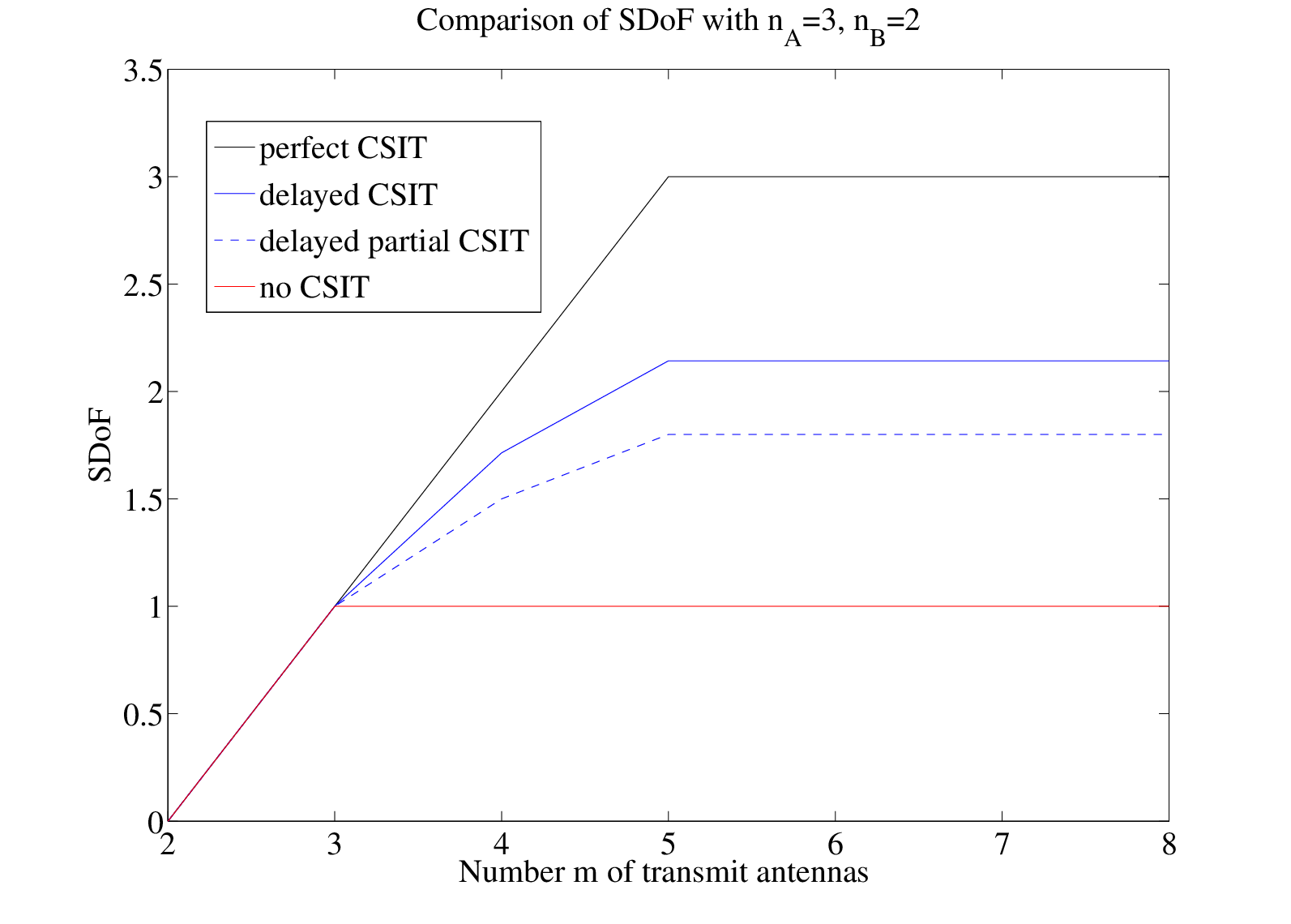
In order to quantify the benefit of delayed CSIT, we summarize the SDoF with perfect, delayed and without CSIT in Table I and provide an example with $n_{\textsf{A}}=3,n_{\textsf{B}}=2$ in Fig. 1. We remark that delayed CSIT is beneficial only when the number of transmit antennas is larger than the number of receive antennas, i.e., $m>\max\{n_{\textsf{A}},n_{\textsf{B}}\}$ , since the SDoF is $(m-n_{\textsf{B}})^{+}$ for $m\leq\max\{n_{\textsf{A}},n_{\textsf{B}}\}$ with perfect, delayed, and without CSIT. As the number $m$ of transmit antennas increases, the SDoF grows until $m=n_{\textsf{A}}+n_{\textsf{B}}$ for perfect and delayed CSIT while it does not increase with $m$ without CSIT. It appears that with both perfect and delayed CSIT, we cannot exploit any gain for $m$ beyond $n_{\textsf{A}}+n_{\textsf{B}}$ . Furthermore, we remark that delayed CSIT only on the legitimate channel incurs a non-negligible loss compared to delayed CSIT on both channels. This is because the transmitter without CSI on the eavesdropper channel cannot access to the signal overheard by the eavesdropper, which reduces the signal dimension to be exploited by the legitimate receiver.

TABLE I: Comparison of the SDoF under different CSIT assumptions for

m>\max\{n_{\textsf{A}},n_{\textsf{B}}\}

CSIT	$\max\{n_{\textsf{A}},n_{\textsf{B}}\}<m<n_{\textsf{A}}+n_{\textsf{B}}$	$m\geq n_{\textsf{A}}+n_{\textsf{B}}$
perfect	$m-n_{\textsf{B}}$	$n_{\textsf{A}}$
delayed	$\frac{n_{\textsf{A}}m(m-n_{\textsf{B}})}{n_{\textsf{A}}n_{\textsf{B}}+m(m-n_{\textsf{B}})}$	$\frac{n_{\textsf{A}}(n_{\textsf{A}}+n_{\textsf{B}})}{n_{\textsf{A}}+2n_{\textsf{B}}}$
delayed partial	$\frac{n_{\textsf{A}}(m-n_{\textsf{B}})}{m}$	$\frac{n_{\textsf{A}}^{2}}{n_{\textsf{A}}+n_{\textsf{B}}}$
no	$(n_{\textsf{A}}-n_{\textsf{B}})^{+}$	$(n_{\textsf{A}}-n_{\textsf{B}})^{+}$

Refer to caption — Fig. 1: SDoF with $n_{\textsf{A}}=3$ and $n_{\textsf{B}}=2$ with perfect, delayed, and no CSIT.

III-B Broadcast channel with confidential messages

Next, we present the achievable SDoF region of the two-user MIMO-BCC with delayed CSIT.

Theorem 3 (BCC with delayed CSIT)

The optimal SDoF region $\mathcal{R}_{\textrm{BCC}}$ of the two-user MIMO-BCC with delayed CSIT is given as a set of non-negative $(d_{\textsf{A}},d_{\textsf{B}})$ satisfying


	$\displaystyle\frac{d_{\textsf{A}}}{d_{s}(n_{\textsf{A}},n_{\textsf{B}},m)}+\frac{d_{\textsf{B}}}{\min\{m,n_{\textsf{A}}+n_{\textsf{B}}\}}\leq 1,$		(15a)
	$\displaystyle\frac{d_{\textsf{A}}}{\min\{m,n_{\textsf{A}}+n_{\textsf{B}}\}}+\frac{d_{\textsf{B}}}{d_{s}(n_{\textsf{B}},n_{\textsf{A}},m)}\leq 1,$		(15b)

for any $m>\max\{n_{\textsf{A}},n_{\textsf{B}}\}$ . If $n_{\textsf{B}}<m\leq n_{\textsf{A}}$ , we have $d_{\textsf{A}}\leq m-n_{\textsf{B}}$ and $d_{\textsf{B}}=0$ , whereas if $n_{\textsf{A}}<m\leq n_{\textsf{B}}$ , we have $d_{\textsf{A}}=0$ and $d_{\textsf{B}}\leq m-n_{\textsf{A}}$ .

Corollary III.1

For the case $m>\max\{n_{\textsf{A}},n_{\textsf{B}}\}$ , the SDoF region is characterized by the two corner points $(0,d_{s}(n_{\textsf{B}},n_{\textsf{A}},m))$ , $(d_{s}(n_{\textsf{A}},n_{\textsf{B}},m),0)$ and the sum SDoF point given by

\displaystyle(d_{\textsf{A}},d_{\textsf{B}})=\begin{cases}\displaystyle{\left(\frac{n_{\textsf{A}}(m-n_{\textsf{B}})}{m},\frac{n_{\textsf{B}}(m-n_{\textsf{A}})}{m}\right)},&\max\{n_{\textsf{A}},n_{\textsf{B}}\}<m\leq{n_{\textsf{A}}+n_{\textsf{B}}}\\ \displaystyle{\left(\frac{n_{\textsf{A}}^{2}}{n_{\textsf{A}}+n_{\textsf{B}}},\frac{n_{\textsf{B}}^{2}}{n_{\textsf{A}}+n_{\textsf{B}}}\right)},&m>n_{\textsf{A}}+n_{\textsf{B}}.\end{cases}

(16)

Remark III.1

We can find trivial upper bounds to the above SDoF region for the case of $m>\max\{n_{\textsf{A}},n_{\textsf{B}}\}$ . On one hand, the SDoF region with delayed CSIT is dominated by the SDoF region with perfect CSIT. The SDoF region with perfect CSIT is square connecting three corner points $(\min\{n_{\textsf{A}},m-n_{\textsf{B}}\},0)$ , $(\min\{n_{\textsf{A}},m-n_{\textsf{B}}\},\min\{m-n_{\textsf{A}},n_{\textsf{B}}\})$ , and $(0,\min\{m-n_{\textsf{A}},n_{\textsf{B}}\})$ . We can also compare the above SDoF region with delayed CSIT and the DoF region of the two-user MIMO-BC with delayed constraint [12], given by


$\displaystyle\frac{d_{\textsf{A}}}{\min\{m,n_{\textsf{A}}\}}+\frac{d_{\textsf{B}}}{\min\{m,n_{\textsf{A}}+n_{\textsf{B}}\}}$	$\displaystyle\leq 1,$	(17a)
$\displaystyle\frac{d_{\textsf{A}}}{\min\{m,n_{\textsf{A}}+n_{\textsf{B}}\}}+\frac{d_{\textsf{B}}}{\min\{m,n_{\textsf{B}}\}}$	$\displaystyle\leq 1.$	(17b)

Obviously, since SDoF is always upper bounded by DoF of the MIMO channel, namely $d_{s}(n_{\textsf{A}},n_{\textsf{B}},m)\leq\min\{n_{\textsf{A}},m\}$ and $d_{s}(n_{\textsf{B}},n_{\textsf{A}},m)\leq\min\{n_{\textsf{B}},m\}$ , the SDoF region is dominated by the DoF region.

We provide an insight to the proposed artificial noise alignment scheme which achieves the sum SDoF point $\left(\frac{1}{2},\frac{1}{2}\right)$ over the two-user MISO-BCC. Let us consider the four-slot scheme where the transmitter sends six independent Gaussian distributed symbols $\boldsymbol{u}\triangleq[u_{1}\ u_{2}]^{\scriptstyle\mathsf{T}}$ , $\boldsymbol{v}_{\textsf{A}}\triangleq[v_{11}\ v_{12}]^{\scriptstyle\mathsf{T}}$ , $\boldsymbol{v}_{\textsf{B}}\triangleq[v_{21}\ v_{22}]^{\scriptstyle\mathsf{T}}$ whose powers scale equally with $P$ . Specifically, the transmit vectors are given by

\displaystyle\boldsymbol{x}_{1}=\boldsymbol{u},\;\;\boldsymbol{x}_{2}=\boldsymbol{v}_{\textsf{A}}+\begin{bmatrix}\boldsymbol{h}_{1}^{{\scriptstyle\mathsf{T}}}\boldsymbol{u}\\ 0\end{bmatrix},\boldsymbol{x}_{3}=\boldsymbol{v}_{\textsf{B}}+\begin{bmatrix}\boldsymbol{g}_{1}^{{\scriptstyle\mathsf{T}}}\boldsymbol{u}\\ 0\end{bmatrix},\boldsymbol{x}_{4}=\begin{bmatrix}(\boldsymbol{g}_{2}^{\scriptstyle\mathsf{T}}\boldsymbol{v}_{\textsf{A}}+g_{21}\boldsymbol{h}_{1}^{{\scriptstyle\mathsf{T}}}\boldsymbol{u})+(\boldsymbol{h}_{3}^{\scriptstyle\mathsf{T}}\boldsymbol{v}_{\textsf{B}}+h_{31}\boldsymbol{g}_{1}^{{\scriptstyle\mathsf{T}}}\boldsymbol{u})\\ 0\end{bmatrix},

(18)

where, for simplicity of demonstration, we omit the scaling factors that fulfill the power constraint (2). Note that this simplification, also adopted in [1] and other related works, does not affect the high SNR analysis carried out here. The following remarks are in order. First, it can be easily shown that, at receiver A, $\boldsymbol{v}_{\textsf{A}}$ lies in a two-dimensional subspace, while the unintended signal $\boldsymbol{v}_{\textsf{B}}$ plus the artificial noise are aligned in another two-dimensional subspace. Thus, the intended message can be recovered through $\boldsymbol{v}_{\textsf{A}}$ from the four-dimensional observation at receiver A. Second, $\boldsymbol{v}_{\textsf{A}}$ is drowned in the observation at receiver B. More precisely, at receiver B, $\boldsymbol{v}_{\textsf{A}}$ is squeezed into a one-dimension subspace filled with artificial noise, which makes it impossible to recover any useful information about A. Due to the symmetry, the same holds for $\boldsymbol{v}_{\textsf{B}}$ . Therefore, we can send simultaneously two confidential symbols to each receiver over four slots, yielding the sum SDoF point $\left(\frac{1}{2},\frac{1}{2}\right)$ .

The four-slot scheme contains two special cases of interest. If we consider the MISO wiretap channel where the transmitter wishes to convey $\boldsymbol{v}_{\textsf{A}}$ to receiver A while keeping it secret to receiver B, we let $\boldsymbol{v}_{\textsf{B}}={\bf 0}$ and ignore the third time slot. This provides a SDoF of $\frac{2}{3}$ . If we consider the two-user MISO-BC without secrecy constraint, we remove the artificial noise transmission by letting $\boldsymbol{u}={\bf 0}$ and ignoring the first time slot. This boils down to the MAT scheme [1]. The four-slot scheme as well as the more general artificial noise alignment scheme presented in Section V is indeed a non-trivial extension of retrospective interference alignment schemes for MIMO broadcast channels [1, 12] to secure communications. The comparison with the three-slot MAT scheme can be interpreted as follows. The messages can be kept secret at a price of an additional resource (one slot), which appears as a DoF loss with respect to the communication systems without secrecy constraint.

In order to visualize the DoF loss due to the secrecy constraints, we provide an example of the achievable DoF/SDoF regions with $m=5$ , $n_{\textsf{A}}=3$ , and $n_{\textsf{B}}=2$ in Fig. 2. For the case of perfect CSIT, the SDoF region and the DoF region are square. In the MIMO-BC, we send $(n_{\textsf{A}}^{2}(n_{\textsf{A}}+n_{\textsf{B}}),n_{\textsf{B}}^{2}(n_{\textsf{A}}+n_{\textsf{B}}))=(45,20)$ private symbols to receiver A and B, respectively, over a duration of $n_{\textsf{A}}^{2}+n_{\textsf{B}}^{2}+n_{\textsf{A}}n_{\textsf{B}}=19$ slots, yielding the DoF $\left(\frac{45}{19},\frac{20}{19}\right)$ , as shown in [12]. Under the perfect secrecy constraints, we need an extra phase of the artificial noise transmission of $n_{\textsf{A}}n_{\textsf{B}}=6$ slots to convey two streams securely. This yields the SDoF of $\left(\frac{9}{5},\frac{4}{5}\right)$ . The comparison with the DoF region of the MIMO-BC can be interpreted in either an optimistic or a pessimistic way. On one hand, the benefit of delayed CSIT is more significant for the SDoF region. On the other hand, we also observe that the lack of accurate CSIT decreases substantially the SDoF, which implies that the secure communications are very sensitive to the quality of CSIT.

IV Wiretap Channel: Proofs of Theorems 1 and 2

IV-A Converse proof of Theorem 1

We are now ready to provide the converse by considering different cases below.

IV-A1 Case $m\leq n_{\textsf{B}}$

From Fano’s inequality and the secrecy constraint, we have

$\displaystyle n(R-\mathsf{o}(\log P))$	$\displaystyle\leq I({{W}};\boldsymbol{{y}}^{n})-I({{W}};\boldsymbol{{z}}^{n})$	(19)
	$\displaystyle=I({{W}};\boldsymbol{{y}}^{n}\,\|\,\boldsymbol{{z}}^{n})-I({{W}};\boldsymbol{{z}}^{n}\,\|\,\boldsymbol{{y}}^{n})$	(20)
	$\displaystyle=h(\boldsymbol{{y}}^{n}\,\|\,\boldsymbol{{z}}^{n})-h(\boldsymbol{{y}}^{n}\,\|\,\boldsymbol{{z}}^{n},{{W}})-I({{W}};\boldsymbol{{z}}^{n}\,\|\,\boldsymbol{{y}}^{n})$	(21)
	$\displaystyle\leq h(\boldsymbol{{y}}^{n}\,\|\,\boldsymbol{{z}}^{n})$	(22)
	$\displaystyle\leq\sum_{t=1}^{n}h(\boldsymbol{{y}}_{t}\,\|\,\boldsymbol{{z}}_{t})$	(23)
	$\displaystyle=\sum_{t=1}^{n}h(\boldsymbol{{y}}_{t}-\boldsymbol{{H}}_{t}\,\hat{\boldsymbol{{x}}}_{\boldsymbol{{z}},t}\,\|\,\boldsymbol{{z}}_{t})$	(24)
	$\displaystyle=\sum_{t=1}^{n}h(\boldsymbol{{e}}_{t}-\boldsymbol{{H}}_{t}\,(\hat{\boldsymbol{{x}}}_{\boldsymbol{{z}},t}-\boldsymbol{{x}}_{t})\,\|\,\boldsymbol{{z}}_{t})$	(25)
	$\displaystyle=\sum_{t=1}^{n}h(\boldsymbol{{e}}_{t}-\boldsymbol{{H}}_{t}\,(\hat{\boldsymbol{{x}}}_{\boldsymbol{{z}},t}-\boldsymbol{{x}}_{t}))$	(26)
	$\displaystyle=n\,\mathsf{o}(\log P),$	(27)

where (22) is from the fact that both $I({{W}};\boldsymbol{{z}}^{n}\,|\,\boldsymbol{{y}}^{n})$ and $h(\boldsymbol{{y}}^{n}\,|\,\boldsymbol{{z}}^{n},{{W}})$ are non-negative; in (24) we use the fact that translations preserve differential entropy and let $\hat{\boldsymbol{{x}}}_{\boldsymbol{{z}},t}$ denote the MMSE estimation of $\boldsymbol{{x}}_{t}$ given $\boldsymbol{{z}}_{t}$ ; the last equality holds because the estimation error does not scale with $P$ .

IV-A2 Case $n_{\textsf{B}}<m\leq\max\left\{n_{\textsf{A}},n_{\textsf{B}}\right\}$

Since this case happens only when $n_{\textsf{B}}<m\leq n_{\textsf{A}}$ , we can assume $m\leq n_{\textsf{A}}$ . Starting from (22), we have

$\displaystyle n(R-\mathsf{o}(\log P))$	$\displaystyle\leq h(\boldsymbol{{y}}^{n}\,\|\,\boldsymbol{{z}}^{n})$	(28)
	$\displaystyle\ \dot{\leq}\ \!\frac{\min\{m,n_{\textsf{A}}+n_{\textsf{B}}\}-n_{\textsf{B}}}{n_{\textsf{B}}}h(\boldsymbol{{z}}^{n})$	(29)
	$\displaystyle\leq n(m-n_{\textsf{B}})\log P+n\,\mathsf{o}(\log P),$	(30)

where (29) follows straightforwardly from (9a); the last inequality comes from the fact that i.i.d. Gaussian variables maximize the differential entropies under the variance constraint.

IV-A3 Case $m>\max\{n_{\textsf{A}},n_{\textsf{B}}\}$

In the following we let $\tilde{m}=\min\{m,n_{\textsf{A}}+n_{\textsf{B}}\}$ for notation simplicity. We remark that two upper bounds can be obtained as a direct consequence of Lemma 1. One one hand, (29) still holds

\displaystyle I({{W}};\boldsymbol{{y}}^{n})-I({{W}};\boldsymbol{{z}}^{n})

\displaystyle\ \dot{\leq}\ \!\frac{\tilde{m}-n_{\textsf{B}}}{n_{\textsf{B}}}h(\boldsymbol{{z}}^{n}).

(31)

On the other hand, we have

$\displaystyle I({{W}};\boldsymbol{{y}}^{n})-I({{W}};\boldsymbol{{z}}^{n})$	$\displaystyle=h(\boldsymbol{{y}}^{n})-h(\boldsymbol{{y}}^{n}\,\|\,{{W}})-h(\boldsymbol{{z}}^{n})+h(\boldsymbol{{z}}^{n}\,\|\,{{W}})$	(32)
	$\displaystyle\ \dot{\leq}\ \!h(\boldsymbol{{y}}^{n})+\left(1-\frac{n_{\textsf{A}}}{\tilde{m}}\right)h(\boldsymbol{{z}}^{n}\,\|\,{{W}})-h(\boldsymbol{{z}}^{n})$	(33)
	$\displaystyle\leq h(\boldsymbol{{y}}^{n})-\frac{n_{\textsf{A}}}{\tilde{m}}h(\boldsymbol{{z}}^{n}),$	(34)

where (33) follows from (9d); (34) follows from $h(\boldsymbol{{z}}^{n}\,|\,W)\leq h(\boldsymbol{{z}}^{n})$ ; By combining the above two upper bounds, we readily have

$\displaystyle n(R-\mathsf{o}(\log P))$	$\displaystyle\leq I({{W}};\boldsymbol{{y}}^{n})-I({{W}};\boldsymbol{{z}}^{n})$	(35)
	$\displaystyle\ \dot{\leq}\ \!\!\min\left\{\frac{\tilde{m}-n_{\textsf{B}}}{n_{\textsf{B}}}h(\boldsymbol{{z}}^{n}),h(\boldsymbol{{y}}^{n})-\frac{n_{\textsf{A}}}{\tilde{m}}h(\boldsymbol{{z}}^{n})\right\}$	(36)
	$\displaystyle\leq\max_{\alpha}\max_{\beta}\min\left\{\frac{\tilde{m}-n_{\textsf{B}}}{n_{\textsf{B}}}\beta,\alpha-\frac{n_{\textsf{A}}}{\tilde{m}}\beta\right\}$	(37)
	$\displaystyle\leq\max_{\alpha}{\alpha}\left({1+\frac{n_{\textsf{A}}n_{\textsf{B}}}{\tilde{m}(\tilde{m}-n_{\textsf{B}})}}\right)^{-1}$	(38)
	$\displaystyle\ \dot{\leq}\ \left({1+\frac{n_{\textsf{A}}n_{\textsf{B}}}{\tilde{m}(\tilde{m}-n_{\textsf{B}})}}\right)^{-1}{n_{\textsf{A}}}n\log P,$	(39)

where (37) is because the RHS of (36) can only increase by maximizing it over both entropies $\alpha=h(\boldsymbol{{y}}^{n}),\beta=h(\boldsymbol{{z}}^{n})$ ; in (38) the inner maximization is solved by equalizing two terms inside $\min$ , and finally we use $h(\boldsymbol{{y}}^{n})\leq n_{\textsf{A}}n\log P+\mathsf{o}(\log P)$ . This establishes the converse proof.

IV-B Achievability proof of Theorem 1

In the following, we wish to show the achievability of the SDoF. As in the converse part, we consider separately the cases for different $m$ . Note that only two ranges of $m$ need to be considered. The first one is $n_{\textsf{B}}\leq m\leq\max\{n_{\textsf{A}},n_{\textsf{B}}\}$ and the other one is $\max\{n_{\textsf{A}},n_{\textsf{B}}\}<m\leq n_{\textsf{A}}+n_{\textsf{B}}$ . For $m<n_{\textsf{B}}$ , the SDoF is zero. For $m>n_{\textsf{A}}+n_{\textsf{B}}$ , the converse shows that it is useless in terms of SDoF to set more than $n_{\textsf{A}}+n_{\textsf{B}}$ antennas.

IV-B1 Case $n_{\textsf{B}}\leq m\leq\max\{n_{\textsf{A}},n_{\textsf{B}}\}$

For this case, we need to show that $d_{s}(n_{\textsf{A}},n_{\textsf{B}},m)=m-n_{\textsf{B}}$ is achievable for $n_{\textsf{B}}<m\leq n_{\textsf{A}}$ . This can be simply done by sending a vector of $m$ symbols of which $m-n_{\textsf{B}}$ symbols $\boldsymbol{{v}}$ are useful message and the other $n_{\textsf{B}}$ symbols $\boldsymbol{{u}}$ are artificial noise (or a random message). The legitimate receiver can decode all $m$ symbols and therefore extract the useful message, i.e.,

$\displaystyle I(\boldsymbol{{v}};\boldsymbol{{y}})$	$\displaystyle=I(\boldsymbol{{v}},\boldsymbol{{u}};\boldsymbol{{y}})-I(\boldsymbol{{u}};\boldsymbol{{y}}\,\|\,\boldsymbol{{v}})$	(40)
	$\displaystyle=\log{\hbox{det}}\left({\bf I}_{n_{\textsf{A}}}+\frac{P}{m}\boldsymbol{H}\boldsymbol{H}^{{\scriptstyle\mathsf{H}}}\right)-\log{\hbox{det}}\left({\bf I}_{n_{\textsf{A}}}+\frac{n_{\textsf{B}}P}{m}\boldsymbol{H}\left[\begin{smallmatrix}{\bf I}_{n_{\textsf{B}}}&\\ &0_{m-n_{\textsf{B}}}\end{smallmatrix}\right]\boldsymbol{H}^{{\scriptstyle\mathsf{H}}}\right)$	(41)
	$\displaystyle\doteq(m-n_{\textsf{B}})\log P,$	(42)

while the eavesdropper channel is inflated by the random message and does not expose more than a vanishing fraction of the useful message, i.e.,

$\displaystyle I(\boldsymbol{{v}};\boldsymbol{{z}})$	$\displaystyle=I(\boldsymbol{{v}},\boldsymbol{{u}};\boldsymbol{{z}})-I(\boldsymbol{{u}};\boldsymbol{{z}}\,\|\,\boldsymbol{{v}})$	(43)
	$\displaystyle=\log{\hbox{det}}\left({\bf I}_{n_{\textsf{B}}}+\frac{P}{m}\boldsymbol{G}\boldsymbol{G}^{{\scriptstyle\mathsf{H}}}\right)-\log{\hbox{det}}\left({\bf I}_{n_{\textsf{B}}}+\frac{n_{\textsf{B}}P}{m}\boldsymbol{G}\left[\begin{smallmatrix}{\bf I}_{n_{\textsf{B}}}&\\ &0_{m-n_{\textsf{B}}}\end{smallmatrix}\right]\boldsymbol{G}^{{\scriptstyle\mathsf{H}}}\right)$	(44)
	$\displaystyle\doteq n_{\textsf{B}}\log P-n_{\textsf{B}}\log P$	(45)
	$\displaystyle=0,$	(46)

where we used the fact that ${\hbox{rank}}(\boldsymbol{H})=m$ and ${\hbox{rank}}(\boldsymbol{G})=n_{\textsf{B}}$ . Note that (41) and (44) are obtained by applying independent Gaussian signaling to $\boldsymbol{{v}}$ and $\boldsymbol{{u}}$ with proper covariance corresponding to the power constraint. This assumption will be implicitly applied in the rest of the paper.

IV-B2 Case $\max\{n_{\textsf{A}},n_{\textsf{B}}\}<m\leq n_{\textsf{A}}+n_{\textsf{B}}$

The proposed scheme combines the artificial noise with the Maddah-Ali Tse (MAT) alignment scheme [1]. The main idea of this scheme is to send the artificial noise such that it fills the eavesdropper’s observation and hides the confidential message, while it shall be aligned in a reduced subspace at the legitimate receiver.

TABLE II: Proposed three-phase scheme for

\max\{n_{\textsf{A}},n_{\textsf{B}}\}<m\leq n_{\textsf{A}}+n_{\textsf{B}}

Phase 1 ( $t\in\mathcal{T}_{1}$ )	Phase 2 ( $t\in\mathcal{T}_{2}$ )	Phase 3 ( $t\in\mathcal{T}_{3}$ )
$\boldsymbol{x}_{1}=\boldsymbol{u}$	$\boldsymbol{x}_{2}=\boldsymbol{v}+{\bf{{\Theta}}}\tilde{\boldsymbol{y}}_{1}$	$\boldsymbol{x}_{3}={\bf{{\Phi}}}\tilde{\boldsymbol{z}}_{2}$
$\tilde{\boldsymbol{y}}_{1}=\tilde{\boldsymbol{H}}_{1}\boldsymbol{u}$	$\tilde{\boldsymbol{y}}_{2}=\tilde{\boldsymbol{H}}_{2}\boldsymbol{v}+\tilde{\boldsymbol{H}}_{2}{\bf{{\Theta}}}\tilde{\boldsymbol{H}}_{1}\boldsymbol{u}$	$\tilde{\boldsymbol{y}}_{3}=\tilde{\boldsymbol{H}}_{3}{\bf{{\Phi}}}\tilde{\boldsymbol{G}}_{2}\boldsymbol{v}+\tilde{\boldsymbol{H}}_{3}{\bf{{\Phi}}}\tilde{\boldsymbol{G}}_{2}{\bf{{\Theta}}}\tilde{\boldsymbol{H}}_{1}\boldsymbol{u}$
$\tilde{\boldsymbol{z}}_{1}=\tilde{\boldsymbol{G}}_{1}\boldsymbol{u}$	$\tilde{\boldsymbol{z}}_{2}=\tilde{\boldsymbol{G}}_{2}\boldsymbol{v}+\tilde{\boldsymbol{G}}_{2}{\bf{{\Theta}}}\tilde{\boldsymbol{H}}_{1}\boldsymbol{u}$	$\tilde{\boldsymbol{z}}_{3}=\tilde{\boldsymbol{G}}_{3}{\bf{{\Phi}}}\tilde{\boldsymbol{G}}_{2}\boldsymbol{v}+\tilde{\boldsymbol{G}}_{3}{\bf{{\Phi}}}\tilde{\boldsymbol{G}}_{2}{\bf{{\Theta}}}\tilde{\boldsymbol{H}}_{1}\boldsymbol{u}$

TABLE III: Length of three phases

\{\tau_{i}\}

for different

m,n_{\textsf{A}},n_{\textsf{B}}

	$\max\{n_{\textsf{A}},n_{\textsf{B}}\}<m\leq n_{\textsf{A}}+n_{\textsf{B}}$	$m>n_{\textsf{A}}+n_{\textsf{B}}$
$\tau_{1}$	$n_{\textsf{A}}n_{\textsf{B}}$	$n_{\textsf{A}}n_{\textsf{B}}$
$\tau_{2}$	$n_{\textsf{A}}(m-n_{\textsf{B}})$	$n_{\textsf{A}}^{2}$
$\tau_{3}$	$(m-n_{\textsf{A}})(m-n_{\textsf{B}})$	$n_{\textsf{A}}n_{\textsf{B}}$
total duration $\sum_{i=1}^{3}\tau_{i}$	$n_{\textsf{A}}n_{\textsf{B}}+m(m-n_{\textsf{B}})$	$2n_{\textsf{A}}n_{\textsf{B}}+n_{\textsf{A}}^{2}$

The proposed three-phase scheme is presented in Table III, where the signal model without thermal noise is described concisely with the block matrix notation:

$\displaystyle\boldsymbol{u}$	$\displaystyle=\bigl[\ \begin{matrix}\boldsymbol{u}_{1}^{\scriptstyle\mathsf{T}}&\dots&\boldsymbol{u}_{\tau_{1}}^{\scriptstyle\mathsf{T}}\end{matrix}\ \bigr]^{\scriptstyle\mathsf{T}}\in\mathbb{C}^{m\tau_{1}\times 1},$	$\displaystyle\boldsymbol{v}$	$\displaystyle=\bigl[\ \begin{matrix}\boldsymbol{v}_{1}^{\scriptstyle\mathsf{T}}&\dots&\boldsymbol{v}_{\tau_{2}}^{\scriptstyle\mathsf{T}}\end{matrix}\ \bigr]^{\scriptstyle\mathsf{T}}\in\mathbb{C}^{m\tau_{2}\times 1},$	(47)
$\displaystyle\tilde{\boldsymbol{H}}_{i}$	$\displaystyle={\hbox{diag}}\left(\{\boldsymbol{H}_{t}\}_{t\in\mathcal{T}_{i}}\right)\in\mathbb{C}^{n_{\textsf{A}}\tau_{i}\times m\tau_{i}},$	$\displaystyle\tilde{\boldsymbol{G}}_{i}$	$\displaystyle={\hbox{diag}}\left(\{\boldsymbol{G}_{t}\}_{t\in\mathcal{T}_{i}}\right)\in\mathbb{C}^{n_{\textsf{B}}\tau_{i}\times m\tau_{i}},$	(48)
$\displaystyle{\bf{{\Theta}}}$	$\displaystyle\in\mathbb{C}^{m\tau_{2}\times n_{\textsf{A}}\tau_{1}},$	$\displaystyle{\bf{{\Phi}}}$	$\displaystyle\in\mbox{\bb C}^{m\tau_{3}\times n_{\textsf{B}}\tau_{2}},$	(49)

where $\tau_{i}$ denotes the length of phase $i$ for $i=1$ , $2$ , and $3$ given in Table III.

The three phases are explained as follows:

•

Phase 1, $t\in\mathcal{T}_{1}\triangleq\{1,\ldots,\tau_{1}\}$ : sending the artificial noise. The $m\tau_{1}$ symbols sent in $\tau_{1}$ time slots is represented by $\boldsymbol{u}$ .
•

Phase 2, $t\in\mathcal{T}_{2}\triangleq\{\tau_{1}+1,\ldots,\tau_{1}+\tau_{2}\}$ : sending the confidential symbols with the artificial noise seen by the legitimate receiver. In $\tau_{2}$ time slots, we send the $m\tau_{2}$ useful symbols represented by $\boldsymbol{v}$ , superimposed by a linear combination (specified by ${\bf{{\Theta}}}$ ) of the artificial noise observed by the legitimate receiver in phase 1.⁴⁴ 4 As mentioned before, we ignore the scaling factor necessary to meet the power constraint. The same holds for the transmit vector in phase 3.
•

Phase 3, $t\in\mathcal{T}_{3}\triangleq\{\tau_{1}+\tau_{2}+1,\ldots,\tau_{1}+\tau_{2}+\tau_{3}\}$ : repeating the eavesdropper’s observation during phase 2. The final phase consists in sending a linear combination (specified by ${\bf{{\Phi}}}$ ) of the eavedropper’s observation in phase 2. The aim of this phase is to complete the equations for the legitimate receiver to solve the useful symbols $\boldsymbol{v}$ without exposing anything new to the eavedropper.

After three phases, the observations are given by


$\displaystyle\boldsymbol{y}$	$\displaystyle=\underbrace{\begin{bmatrix}{\bf I}_{n_{\textsf{A}}\tau_{1}}&{\bf 0}_{m\tau_{2}}\\ \tilde{\boldsymbol{H}}_{2}{\bf{{\Theta}}}&\tilde{\boldsymbol{H}}_{2}\\ \tilde{\boldsymbol{H}}_{3}{\bf{{\Phi}}}\tilde{\boldsymbol{G}}_{2}{\bf{{\Theta}}}&\tilde{\boldsymbol{H}}_{3}{\bf{{\Phi}}}\tilde{\boldsymbol{G}}_{2}\end{bmatrix}}_{\boldsymbol{\mathsf{\widehat{H}}}}\begin{bmatrix}\tilde{\boldsymbol{H}}_{1}\boldsymbol{u}\\ \boldsymbol{v}\end{bmatrix}+\boldsymbol{e},$	(50a)
$\displaystyle\boldsymbol{z}$	$\displaystyle=\underbrace{\begin{bmatrix}\tilde{\boldsymbol{G}}_{1}&{\bf 0}_{n_{\textsf{B}}\tau_{2}}\\ \tilde{\boldsymbol{G}}_{2}{\bf{{\Theta}}}\tilde{\boldsymbol{H}}_{1}&{\bf I}_{n_{\textsf{B}}\tau_{2}}\\ \tilde{\boldsymbol{G}}_{3}{\bf{{\Phi}}}\tilde{\boldsymbol{G}}_{2}{\bf{{\Theta}}}\tilde{\boldsymbol{H}}_{1}&\tilde{\boldsymbol{G}}_{3}{\bf{{\Phi}}}\end{bmatrix}}_{\boldsymbol{\mathsf{\widehat{G}}}}\begin{bmatrix}\boldsymbol{u}\\ \tilde{\boldsymbol{G}}_{2}\boldsymbol{v}\end{bmatrix}+\boldsymbol{b}.$	(50b)

Therefore, we have

$\displaystyle I(\boldsymbol{{v}};\boldsymbol{{y}})$	$\displaystyle=I(\boldsymbol{{v}},\tilde{\boldsymbol{H}}_{1}\boldsymbol{{u}};\boldsymbol{{y}})-I(\tilde{\boldsymbol{H}}_{1}\boldsymbol{{u}};\boldsymbol{{y}}\,\|\,\boldsymbol{{v}})$	(51)
	$\displaystyle\doteq{\hbox{rank}}\bigl(\boldsymbol{\mathsf{\widehat{H}}}\bigr)\log(P)-{\hbox{rank}}\left(\begin{smallmatrix}{\bf I}_{n_{\textsf{A}}\tau_{1}}\\ \tilde{\boldsymbol{H}}_{2}{\bf{{\Theta}}}\\ \tilde{\boldsymbol{H}}_{3}{\bf{{\Phi}}}\tilde{\boldsymbol{G}}_{2}{\bf{{\Theta}}}\end{smallmatrix}\right)\log(P)$	(52)
	$\displaystyle=\left(n_{\textsf{A}}\tau_{1}+{\hbox{rank}}\left(\begin{smallmatrix}\tilde{\boldsymbol{H}}_{2}\\ \tilde{\boldsymbol{H}}_{3}{\bf{{\Phi}}}\tilde{\boldsymbol{G}}_{2}\end{smallmatrix}\right)\right)\log(P)-n_{\textsf{A}}\tau_{1}\log P$	(53)
	$\displaystyle={\hbox{rank}}\left(\begin{smallmatrix}\tilde{\boldsymbol{H}}_{2}\\ \tilde{\boldsymbol{H}}_{3}{\bf{{\Phi}}}\tilde{\boldsymbol{G}}_{2}\end{smallmatrix}\right)\log(P)$	(54)
	$\displaystyle=mn_{\textsf{A}}(m-n_{\textsf{B}})\log P,$	(55)

where (53) follows due to the block-triangular structure of $\boldsymbol{\mathsf{\widehat{H}}}$ and by the fact that the rank of the second term corresponds to the rank of the identity matrix. In order to prove the last equality, we need to show first that the submatrix $\tilde{\boldsymbol{H}}_{3}{\bf{{\Phi}}}\tilde{\boldsymbol{G}}_{2}$ has full-row rank with linearly independent $n_{\textsf{A}}\tau_{3}$ rows. This is satisfied by letting

\displaystyle{\bf{{\Phi}}}\boldsymbol{\Pi}=\begin{bmatrix}{\hbox{diag}}(\{{\bf{{\Phi}}}_{t}\}_{t=1}^{\tau_{3}})&{\bf 0}_{m\tau_{3}\times(n_{\textsf{B}}\tau_{2}-n_{\textsf{A}}\tau_{3})}\end{bmatrix},

(56)

where $\boldsymbol{\Pi}$ is a permutation matrix such that the first $n_{\textsf{A}}\tau_{3}$ rows of $\boldsymbol{\Pi}^{\scriptstyle\mathsf{T}}\tilde{\boldsymbol{G}}_{2}$ , is block diagonal, denoted by ${\hbox{diag}}\left(\{\boldsymbol{G}_{2,t}^{\Pi}\}_{t\in{\cal T}_{2}}\right)$ , where $\boldsymbol{G}_{2,t}^{\Pi}\in\mbox{\bb C}^{(m-n_{\textsf{A}})\times m}$ is a submatrix of $\tilde{\boldsymbol{G}}_{2,t}$ ; ${\bf{{\Phi}}}_{t}$ denotes a $m\times n_{\textsf{A}}$ matrix with $n_{\textsf{A}}$ independent columns, e.g., ${\bf{{\Phi}}}_{t}=\bigl[\begin{matrix}{\bf I}_{n_{\textsf{A}}}&{\bf 0}_{n_{\textsf{A}}\times(m-n_{\textsf{A}})}\end{matrix}\bigr]^{\scriptstyle\mathsf{T}}$ . Note that with this particular choice of ${\bf{{\Phi}}}$ , the resulting submatrix is given by

\displaystyle\tilde{\boldsymbol{H}}_{3}{\bf{{\Phi}}}\tilde{\boldsymbol{G}}_{2}={\hbox{diag}}(\{\boldsymbol{H}_{t+\tau_{1}+\tau_{2}}{\bf{{\Phi}}}_{t}\}_{t=1}^{\tau_{3}})\,{\hbox{diag}}\left(\{\boldsymbol{G}_{2,t}^{\Pi}\}_{t\in{\cal T}_{2}}\right)

(57)

Since the first matrix in the right hand side of (57) is square and full-rank, it is easy to see that ${\hbox{rank}}\left(\begin{smallmatrix}\tilde{\boldsymbol{H}}_{2}\\ \tilde{\boldsymbol{H}}_{3}{\bf{{\Phi}}}\tilde{\boldsymbol{G}}_{2}\end{smallmatrix}\right)={\hbox{rank}}\left(\begin{smallmatrix}\tilde{\boldsymbol{H}}_{2}\\ {\hbox{diag}}\left(\{\boldsymbol{G}_{2,t}^{\Pi}\}_{t\in{\cal T}_{2}}\right)\end{smallmatrix}\right)$ . By the row permutation, we can readily show that the latter has a desired rank of $mn_{\textsf{A}}(m-n_{\textsf{B}})$ . Namely,

	$\displaystyle{\hbox{rank}}\left(\begin{matrix}\tilde{\boldsymbol{H}}_{2}\\ {\hbox{diag}}\left(\{\boldsymbol{G}_{2,t}^{\Pi}\}_{t\in{\cal T}_{2}}\right)\end{matrix}\right)$	$\displaystyle=\sum_{t=1}^{n_{\textsf{A}}(m-n_{\textsf{B}})}{\hbox{rank}}\left(\begin{matrix}\tilde{\boldsymbol{H}}_{2,t}\\ \tilde{\boldsymbol{G}}_{2,t}^{\Pi}\end{matrix}\right)$		(58)
		$\displaystyle=n_{\textsf{A}}(m-n_{\textsf{B}})m,$		(59)

where the last equality follows by noticing that each block $t$ corresponds to $m$ different rows of the state matrix $\boldsymbol{S}_{t}$ which are linearly independent from Assumption II.2. On the other hand, the eavesdropper’s observation is filled by the artificial noise and thus does not expose more than a vanishing fraction of the useful message, i.e.,

$\displaystyle I(\boldsymbol{{v}};\boldsymbol{{z}})$	$\displaystyle\leq I(\tilde{\boldsymbol{G}}_{2}\boldsymbol{{v}};\boldsymbol{{z}})$	(60)
	$\displaystyle=I(\tilde{\boldsymbol{G}}_{2}\boldsymbol{{v}},\boldsymbol{{u}};\boldsymbol{{z}})-I(\boldsymbol{{u}};\boldsymbol{{z}}\,\|\,\tilde{\boldsymbol{G}}_{2}\boldsymbol{{v}})$	(61)
	$\displaystyle\doteq n_{\textsf{B}}(\tau_{1}+\tau_{2})\log P-{\hbox{rank}}\left(\begin{smallmatrix}\tilde{\boldsymbol{G}}_{1}\\ \tilde{\boldsymbol{G}}_{2}{\bf{{\Theta}}}\tilde{\boldsymbol{H}}_{1}\\ \tilde{\boldsymbol{G}}_{3}\boldsymbol{B}\tilde{\boldsymbol{G}}_{2}{\bf{{\Theta}}}\tilde{\boldsymbol{H}}_{1}\end{smallmatrix}\right)\log P$	(62)
	$\displaystyle=mn_{\textsf{A}}n_{\textsf{B}}\log P-{\hbox{rank}}\left(\begin{smallmatrix}\tilde{\boldsymbol{G}}_{1}\\ \tilde{\boldsymbol{G}}_{2}{\bf{{\Theta}}}\tilde{\boldsymbol{H}}_{1}\end{smallmatrix}\right)\log P$	(63)
	$\displaystyle\doteq 0,$	(64)

where (60) follows due to the Markov chain $\boldsymbol{{v}}\leftrightarrow\tilde{\boldsymbol{G}}_{2}\boldsymbol{{v}}\leftrightarrow\boldsymbol{{z}}$ ; (62) follows by noticing that the rank of $\boldsymbol{\mathsf{\widehat{G}}}$ is determined by the submatrix corresponding to first two phases; (63) follows because the third block row is a linear combination of rows from the second block row. In order to prove the last equality, we choose

\displaystyle{\bf{{\Theta}}}\boldsymbol{\Pi}=\begin{bmatrix}{\hbox{diag}}(\{{\bf{{\Theta}}}_{t}\}_{t=1}^{\tau_{2}})&{\bf 0}_{m\tau_{1}\times(n_{\textsf{A}}\tau_{1}-n_{\textsf{B}}\tau_{2})}\end{bmatrix},

(65)

where $\boldsymbol{\Pi}$ is a permutation matrix⁵⁵ 5 We abuse the notation to denote another permutation matrix than the one used in (56) . such that the first $n_{\textsf{B}}\tau_{2}$ rows of $\boldsymbol{\Pi}^{\scriptstyle\mathsf{T}}\tilde{\boldsymbol{H}}_{1}$ is block diagonal, denoted by ${\hbox{diag}}\left(\{\tilde{\boldsymbol{H}}_{1,t}^{\Pi}\}_{t\in{\cal T}_{1}}\right)$ , with $\tilde{\boldsymbol{H}}_{1,t}^{\Pi}$ being a $(m-n_{\textsf{B}})\times m$ submatrix of $\tilde{\boldsymbol{H}}_{1,t}$ ; ${\bf{{\Theta}}}_{t}$ denotes a $m\times n_{\textsf{B}}$ matrix with $n_{\textsf{B}}$ independent columns, e.g., ${\bf{{\Theta}}}_{t}=\bigl[\begin{matrix}{\bf I}_{n_{\textsf{B}}}&{\bf 0}_{n_{\textsf{B}}\times(m-n_{\textsf{B}})}\end{matrix}\bigr]^{\scriptstyle\mathsf{T}}$ . By applying exactly the same reasoning as on the choice of ${\bf{{\Phi}}}$ , we can prove that ${\hbox{rank}}\left(\begin{smallmatrix}\tilde{\boldsymbol{G}}_{1}\\ \tilde{\boldsymbol{G}}_{2}{\bf{{\Theta}}}\tilde{\boldsymbol{H}}_{1}\end{smallmatrix}\right)=m\tau_{1}=mn_{\textsf{A}}n_{\textsf{B}}$ . As a result, the $n_{\textsf{A}}m(m-n_{\textsf{B}})$ useful symbols can be conveyed secretly over $n_{\textsf{A}}n_{\textsf{B}}+m(m-n_{\textsf{B}})$ time slots in the high SNR regime, yielding the SDoF of $\frac{n_{\textsf{A}}m(m-n_{\textsf{B}})}{n_{\textsf{A}}n_{\textsf{B}}+m(m-n_{\textsf{B}})}$ .

IV-C Achievability proof of Theorem 2

In this subsection, we provide the achievability proof for the case of delayed partial CSIT when the transmitter has delayed CSI only on the legitimate channel. We focus on the case $\max\{n_{\textsf{A}},n_{\textsf{B}}\}<m<n_{\textsf{A}}+n_{\textsf{B}}$ . For the case of $m\geq n_{\textsf{A}}+n_{\textsf{B}}$ , we can easily show that the desired SDoF follows by using only $n_{\textsf{A}}+n_{\textsf{B}}$ antennas out of $m$ , i.e., by replacing $m$ by $n_{\textsf{A}}+n_{\textsf{B}}$ similarly to the case of delayed CSIT on both channels. We propose a variant of the artificial noise alignment scheme described previously. The lack of CSIT on the eavesdropper channel requires the following modifications. First, the transmission consists of first two phases presented in Table III, because the lack of CSI on the eavesdropper channel does not enable the transmitter to repeat the signal overheard by the eavesdropper (corresponding to the third phase). Consequently, the confidential symbols $\boldsymbol{v}$ sent during the second phase must be decoded within this phase. This decreases the dimension of $\boldsymbol{v}$ from $m\tau_{2}$ to $n_{\textsf{A}}\tau_{2}$ . After two phases, the observations are given by


$\displaystyle\boldsymbol{y}$	$\displaystyle=\underbrace{\begin{bmatrix}{\bf I}_{n_{\textsf{A}}\tau_{1}}&{\bf 0}_{n_{\textsf{A}}\tau_{2}}\\ \tilde{\boldsymbol{H}}_{2}{\bf{{\Theta}}}&\tilde{\boldsymbol{H}}_{2}\\ \end{bmatrix}}_{\boldsymbol{\mathsf{\widehat{H}}}}\begin{bmatrix}\tilde{\boldsymbol{H}}_{1}\boldsymbol{u}\\ \boldsymbol{v}\end{bmatrix}+\boldsymbol{e},$	(66a)
$\displaystyle\boldsymbol{z}$	$\displaystyle=\underbrace{\begin{bmatrix}\tilde{\boldsymbol{G}}_{1}&{\bf 0}_{n_{\textsf{B}}\tau_{2}}\\ \tilde{\boldsymbol{G}}_{2}{\bf{{\Theta}}}\tilde{\boldsymbol{H}}_{1}&{\bf I}_{n_{\textsf{B}}\tau_{2}}\\ \end{bmatrix}}_{\boldsymbol{\mathsf{\widehat{G}}}}\begin{bmatrix}\boldsymbol{u}\\ \tilde{\boldsymbol{G}}_{2}\boldsymbol{v}\end{bmatrix}+\boldsymbol{b}.$	(66b)

Following similar steps as before and choosing ${\bf{{\Theta}}}$ in (65), we can easily show that

	$\displaystyle I(\boldsymbol{{v}};\boldsymbol{{y}})$	$\displaystyle\doteq n_{\textsf{A}}^{2}(m-n_{\textsf{B}})\log P,$		(67)
	$\displaystyle I(\boldsymbol{{v}};\boldsymbol{{z}})$	$\displaystyle\doteq 0.$		(68)

As a result, the $n_{\textsf{A}}^{2}(m-n_{\textsf{B}})$ useful symbols can be conveyed secretly over $n_{\textsf{A}}m$ time slots in the high SNR regime, yielding the SDoF of $\frac{n_{\textsf{A}}(m-n_{\textsf{B}})}{m}$ .

V Broadcast Channel with Confidential Messages: Proof of Theorem 3

V-A Converse

We focus on the case $m>\max\{n_{\textsf{A}},n_{\textsf{B}}\}$ in the following. The converse for the other cases is trivial from Section IV. The secrecy constraint (5) together with Fano’s inequality for ${{W}}_{\textsf{B}}$ , i.e., $h({{W}}_{\textsf{B}}|\boldsymbol{z}^{n})\leq n\epsilon$ , yields

I({{W}}_{\textsf{A}};\boldsymbol{{z}}^{n}|{{W}}_{\textsf{B}})\leq n\,\mathsf{o}(\log P).

(69)

Similarly to the converse of the MIMO wiretap channel, we obtain two upper bounds on $R_{\textsf{A}}$ . The first bound is obtained by combining (69) with Fano’s inequality on ${{W}}_{\textsf{A}}$ , i.e., $h({{W}}_{\textsf{A}}|\boldsymbol{y}^{n})\leq n\epsilon$ ,

$\displaystyle n(R_{\textsf{A}}-\mathsf{o}(\log P))$	$\displaystyle\leq I({{W}}_{\textsf{A}};\boldsymbol{{y}}^{n}\|{{W}}_{\textsf{B}})-I({{W}}_{\textsf{A}};\boldsymbol{{z}}^{n}\|{{W}}_{\textsf{B}})$
	$\displaystyle\leq I({{W}}_{\textsf{A}};\boldsymbol{{y}}^{n}\|\boldsymbol{{z}}^{n},{{W}}_{\textsf{B}})$	(70)
	$\displaystyle\leq h(\boldsymbol{{y}}^{n}\|\boldsymbol{{z}}^{n},{{W}}_{\textsf{B}})$	(71)
	$\displaystyle\ \dot{\leq}\ \frac{\tilde{m}-n_{\textsf{B}}}{n_{\textsf{B}}}h(\boldsymbol{{z}}^{n}\|{{W}}_{\textsf{B}}),$	(72)

where (70) follows by $I({{W}}_{\textsf{A}};\boldsymbol{{y}}^{n}|{{W}}_{\textsf{B}})\leq I({{W}}_{\textsf{A}};\boldsymbol{{y}}^{n},\boldsymbol{{z}}^{n}|{{W}}_{\textsf{B}})$ ; (72) follows from inequality (9a) in Lemma 1. The second bound is (34) which holds also here by replacing ${{W}}$ by ${{W}}_{\textsf{A}}$ , namely,

\displaystyle I({{W}}_{\textsf{A}};\boldsymbol{{y}}^{n})-I({{W}}_{\textsf{A}};\boldsymbol{{z}}^{n})\ \dot{\leq}\ h(\boldsymbol{{y}}^{n})-\frac{n_{\textsf{A}}}{\tilde{m}}h(\boldsymbol{{z}}^{n}).

(73)

Putting the two upper bounds together, we have

n(R_{\textsf{A}}-\mathsf{o}(\log P))\ \dot{\leq}\ \min\left\{\frac{\tilde{m}-n_{\textsf{B}}}{n_{\textsf{B}}}h(\boldsymbol{{z}}^{n}|{{W}}_{\textsf{B}}),h(\boldsymbol{{y}}^{n})-\frac{n_{\textsf{A}}}{\tilde{m}}h(\boldsymbol{{z}}^{n})\right\}.

(74)

On the other hand, Fano’s inequality for ${{W}}_{\textsf{B}}$ leads to

n(R_{\textsf{B}}-\mathsf{o}(\log P))\leq h(\boldsymbol{{z}}^{n})-h(\boldsymbol{{z}}^{n}|{{W}}_{\textsf{B}}).

(75)

Now, we sum inequalities (74) and (75) with the weight $T_{\textsf{A}}=n_{\textsf{A}}n_{\textsf{B}}+\tilde{m}(\tilde{m}-n_{\textsf{B}})$ , $n_{\textsf{A}}(\tilde{m}-n_{\textsf{B}})$ , respectively. This yields

$\displaystyle n(T_{\textsf{A}}R_{\textsf{A}}+n_{\textsf{A}}(\tilde{m}-n_{\textsf{B}})R_{\textsf{B}}-\mathsf{o}(\log P))$	$\displaystyle\ \dot{\leq}\ \!\max_{h(\boldsymbol{{y}}^{n})}\max_{\alpha}\min\left\{(\tilde{m}-n_{\textsf{B}})\alpha,T_{\textsf{A}}h(\boldsymbol{{y}}^{n})-\frac{n_{\textsf{A}}n_{\textsf{B}}}{\tilde{m}}\alpha\right\}$	(76)
	$\displaystyle\leq\max_{h(\boldsymbol{{y}}^{n})}\tilde{m}(\tilde{m}-n_{\textsf{B}})h(\boldsymbol{{y}}^{n})$	(77)
	$\displaystyle\ \dot{\leq}\ \!n_{\textsf{A}}\tilde{m}(\tilde{m}-n_{\textsf{B}})n\log P,$	(78)

where we let $\alpha=n_{\textsf{A}}h(\boldsymbol{{z}}^{n})+\frac{\tilde{m}(\tilde{m}-n_{\textsf{B}})}{n_{\textsf{B}}}h(\boldsymbol{{z}}^{n}|{{W}}_{\textsf{B}})$ in the first inequality and the last inequality follows because $h(\boldsymbol{{y}}^{n})\leq nn_{\textsf{A}}\log P+\mathsf{o}(\log P)$ . By dividing both sides by $n_{\textsf{A}}\tilde{m}(\tilde{m}-n_{\textsf{B}})\log P$ and letting $P$ grow, we obtain the first desired inequality (15a). Due to the symmetry of the problem, (15b) can be obtained by swapping the roles of $R_{\textsf{A}}$ and $R_{\textsf{B}}$ . This completes the converse proof.

V-B Achievability

TABLE IV: Proposed four-phase scheme for

\max\{n_{\textsf{A}},n_{\textsf{B}}\}<m\leq n_{\textsf{A}}+n_{\textsf{B}}

Phase 1	Phase 2	Phase 3
$\boldsymbol{x}_{1}=\boldsymbol{u}$	$\boldsymbol{x}_{2}=\boldsymbol{v}_{\textsf{A}}+{\bf{{\Theta}}}_{\textsf{A}}\tilde{\boldsymbol{y}}_{1}$	$\boldsymbol{x}_{3}=\boldsymbol{v}_{\textsf{B}}+{\bf{{\Theta}}}_{\textsf{B}}\tilde{\boldsymbol{z}}_{1}$
$\tilde{\boldsymbol{y}}_{1}=\tilde{\boldsymbol{H}}_{1}\boldsymbol{u}$	$\tilde{\boldsymbol{y}}_{2}=\tilde{\boldsymbol{H}}_{2}\left(\boldsymbol{v}_{\textsf{A}}+{\bf{{\Theta}}}_{\textsf{A}}\tilde{\boldsymbol{H}}_{1}\boldsymbol{u}\right)$	$\tilde{\boldsymbol{y}}_{3}=\tilde{\boldsymbol{H}}_{3}\left(\boldsymbol{v}_{\textsf{B}}+{\bf{{\Theta}}}_{\textsf{B}}\tilde{\boldsymbol{G}}_{1}\boldsymbol{u}\right)$
$\tilde{\boldsymbol{z}}_{1}=\tilde{\boldsymbol{G}}_{1}\boldsymbol{u}$	$\tilde{\boldsymbol{z}}_{2}=\tilde{\boldsymbol{G}}_{2}\left(\boldsymbol{v}_{\textsf{A}}+{\bf{{\Theta}}}_{\textsf{A}}\tilde{\boldsymbol{H}}_{1}\boldsymbol{u}\right)$	$\tilde{\boldsymbol{z}}_{3}=\tilde{\boldsymbol{G}}_{3}\left(\boldsymbol{v}_{\textsf{B}}+{\bf{{\Theta}}}_{\textsf{B}}\tilde{\boldsymbol{G}}_{1}\boldsymbol{u}\right)$
Phase 4
$\boldsymbol{x}_{4}={\bf{{\Phi}}}_{\textsf{A}}\tilde{\boldsymbol{z}}_{2}+{\bf{{\Phi}}}_{\textsf{B}}\tilde{\boldsymbol{y}}_{3}$
$\tilde{\boldsymbol{y}}_{4}=\tilde{\boldsymbol{H}}_{4}{\bf{{\Phi}}}_{\textsf{A}}(\tilde{\boldsymbol{G}}_{2}\boldsymbol{v}_{\textsf{A}}+\tilde{\boldsymbol{G}}_{2}{\bf{{\Theta}}}_{\textsf{A}}\tilde{\boldsymbol{H}}_{1}\boldsymbol{u})+\tilde{\boldsymbol{H}}_{4}{\bf{{\Phi}}}_{\textsf{B}}(\tilde{\boldsymbol{H}}_{3}\boldsymbol{v}_{\textsf{B}}+\tilde{\boldsymbol{H}}_{3}{\bf{{\Theta}}}_{\textsf{B}}\tilde{\boldsymbol{G}}_{1}\boldsymbol{u})$
$\tilde{\boldsymbol{z}}_{4}=\tilde{\boldsymbol{G}}_{4}{\bf{{\Phi}}}_{\textsf{A}}(\tilde{\boldsymbol{G}}_{2}\boldsymbol{v}_{\textsf{A}}+\tilde{\boldsymbol{G}}_{2}{\bf{{\Theta}}}_{\textsf{A}}\tilde{\boldsymbol{H}}_{1}\boldsymbol{u})+\tilde{\boldsymbol{G}}_{4}{\bf{{\Phi}}}_{\textsf{B}}(\tilde{\boldsymbol{H}}_{3}\boldsymbol{v}_{\textsf{B}}+\tilde{\boldsymbol{H}}_{3}{\bf{{\Theta}}}_{\textsf{B}}\tilde{\boldsymbol{G}}_{1}\boldsymbol{u})$

TABLE V: Length of four phases

\{\tau_{i}\}

for different

m

n_{\textsf{A}}

, and

n_{\textsf{B}}

	$\max\{n_{\textsf{A}},n_{\textsf{B}}\}<m\leq n_{\textsf{A}}+n_{\textsf{B}}$	$m>n_{\textsf{A}}+n_{\textsf{B}}$
$\tau_{1}$	$n_{\textsf{A}}n_{\textsf{B}}$	$n_{\textsf{A}}n_{\textsf{B}}$
$\tau_{2}$	$n_{\textsf{A}}(m-n_{\textsf{B}})$	$n_{\textsf{A}}^{2}$
$\tau_{3}$	$n_{\textsf{B}}(m-n_{\textsf{A}})$	$n_{\textsf{B}}^{2}$
$\tau_{4}$	$(m-n_{\textsf{A}})(m-n_{\textsf{B}})$	$n_{\textsf{A}}n_{\textsf{B}}$
total duration $\sum_{i=1}^{4}\tau_{i}$	$m^{2}$	$(n_{\textsf{A}}+n_{\textsf{B}})^{2}$

The corner points can be achieved by the ANA scheme described in Section IV. Here, we provide a strategy achieving the sum SDoF point. In fact, the ANA scheme for the MIMO wiretap channel in Section IV can be suitably modified to convey two confidential messages. We focus on the case $\max\{n_{\textsf{A}},n_{\textsf{B}}\}<m\leq n_{\textsf{A}}+n_{\textsf{B}}$ because the converse proof says that we only need to use $n_{\textsf{A}}+n_{\textsf{B}}$ antennas for the case $m>n_{\textsf{A}}+n_{\textsf{B}}$ .

The proposed four-phase scheme is presented in Table V, where the signal model is describe concisely with the block matrix notation:

$\displaystyle\boldsymbol{u}$	$\displaystyle=\bigl[\ \begin{matrix}\boldsymbol{u}_{1}^{\scriptstyle\mathsf{T}}&\dots&\boldsymbol{u}_{\tau_{1}}^{\scriptstyle\mathsf{T}}\end{matrix}\ \bigr]^{\scriptstyle\mathsf{T}}\in\mathbb{C}^{m\tau_{1}\times 1},$			(79)
$\displaystyle\boldsymbol{v}_{\textsf{A}}$	$\displaystyle=\bigl[\ \begin{matrix}\boldsymbol{v}_{\textsf{A},1}^{\scriptstyle\mathsf{T}}&\dots&\boldsymbol{v}_{\textsf{A},\tau_{2}}^{\scriptstyle\mathsf{T}}\end{matrix}\ \bigr]^{\scriptstyle\mathsf{T}}\in\mathbb{C}^{m\tau_{2}\times 1},$	$\displaystyle\boldsymbol{v}_{\textsf{B}}$	$\displaystyle=\bigl[\ \begin{matrix}\boldsymbol{v}_{\textsf{B},1}^{\scriptstyle\mathsf{T}}&\dots&\boldsymbol{v}_{\textsf{B},\tau_{3}}^{\scriptstyle\mathsf{T}}\end{matrix}\ \bigr]^{\scriptstyle\mathsf{T}}\in\mathbb{C}^{m\tau_{3}\times 1},$	(80)
$\displaystyle\tilde{\boldsymbol{H}}_{i}$	$\displaystyle={\hbox{diag}}\left(\{\boldsymbol{H}_{t}\}_{t\in\mathcal{T}_{i}}\right)\in\mathbb{C}^{n_{\textsf{A}}\tau_{i}\times m\tau_{i}},$	$\displaystyle\tilde{\boldsymbol{G}}_{i}$	$\displaystyle={\hbox{diag}}\left(\{\boldsymbol{G}_{t}\}_{t\in\mathcal{T}_{i}}\right)\in\mathbb{C}^{n_{\textsf{B}}\tau_{i}\times m\tau_{i}},$	(81)
$\displaystyle{\bf{{\Theta}}}_{\textsf{A}}$	$\displaystyle\in\mathbb{C}^{m\tau_{2}\times n_{\textsf{A}}\tau_{1}},$	$\displaystyle{\bf{{\Theta}}}_{\textsf{B}}$	$\displaystyle\in\mathbb{C}^{m\tau_{3}\times n_{\textsf{B}}\tau_{1}},$	(82)
$\displaystyle{\bf{{\Phi}}}_{\textsf{A}}$	$\displaystyle\in\mbox{\bb C}^{m\tau_{4}\times n_{\textsf{B}}\tau_{2}},$	$\displaystyle{\bf{{\Phi}}}_{\textsf{B}}$	$\displaystyle\in\mbox{\bb C}^{m\tau_{4}\times n_{\textsf{A}}\tau_{3}},$	(83)

where the durations of four phases $\{\tau_{i}\}_{i}$ are given in Table V. The four phases consist of:

•

Phase 1, $t\in\mathcal{T}_{1}\triangleq\{1,\ldots,\tau_{1}\}$ : sending the artificial noise. The $m\tau_{1}$ symbols sent in $\tau_{1}$ time slots is represented by $\boldsymbol{u}$ .
•

Phase 2, $t\in\mathcal{T}_{2}\triangleq\{\tau_{1}+1,\ldots,\tau_{1}+\tau_{2}\}$ : sending the confidential symbols $\boldsymbol{v}_{\textsf{A}}$ with the artificial noise seen by receiver A. In $\tau_{2}$ time slots, we send the $m\tau_{2}$ useful symbols represented by $\boldsymbol{v}_{\textsf{A}}$ , superimposed by a linear combination (specified by ${\bf{{\Theta}}}_{\textsf{A}}$ ) of the artificial noise observed by receiver A in phase 1.
•

Phase 3, $t\in\mathcal{T}_{3}\triangleq\{\tau_{1}+\tau_{2}+1,\ldots,\tau_{1}+\tau_{2}+\tau_{3}\}$ : sending the confidential symbols $\boldsymbol{v}_{\textsf{B}}$ with the artificial noise seen by receiver B. In $\tau_{3}$ time slots, we send the $m\tau_{3}$ useful symbols represented by $\boldsymbol{v}_{\textsf{B}}$ , superimposed by a linear combination (specified by ${\bf{{\Theta}}}_{\textsf{B}}$ ) of the artificial noise observed by receiver B in phase 1.
•

Phase 4, $t\in\mathcal{T}_{4}\triangleq\{\tau_{1}+\tau_{2}+\tau_{3}+1,\ldots,\tau_{1}+\tau_{2}+\tau_{3}+\tau_{4}\}$ : repeating the past observations during in phase 2 and 3. The final phase consists in sending a linear combination of receiver B’s observation in phase 2 (specified by ${\bf{{\Phi}}}_{\textsf{A}}$ ) and receiver A’s observation in phase 3 (specified by ${\bf{{\Phi}}}_{\textsf{B}}$ ). The aim of this phase is to complete the equations for the intended receivers to solve the useful symbols without exposing anything new about the message to the unintended receivers.

After four phases, the observations are given by


$\displaystyle\boldsymbol{y}$	$\displaystyle=\underbrace{\begin{bmatrix}\tilde{\boldsymbol{H}}_{2}&\tilde{\boldsymbol{H}}_{2}{\bf{{\Theta}}}_{\textsf{A}}&{\bf 0}\\ \tilde{\boldsymbol{H}}_{4}{\bf{{\Phi}}}_{\textsf{A}}\tilde{\boldsymbol{G}}_{2}&\tilde{\boldsymbol{H}}_{4}{\bf{{\Phi}}}_{\textsf{A}}\tilde{\boldsymbol{G}}_{2}{\bf{{\Theta}}}_{\textsf{A}}&\tilde{\boldsymbol{H}}_{4}\\ {\bf 0}&{\bf I}_{n_{\textsf{A}}\tau_{1}}&{\bf 0}\\ {\bf 0}&{\bf 0}&{\bf I}_{n_{\textsf{A}}\tau_{3}}\end{bmatrix}}_{\boldsymbol{\mathsf{\widehat{H}}}_{\text{bcc}}}\begin{bmatrix}\boldsymbol{v}_{\textsf{A}}\\ \tilde{\boldsymbol{H}}_{1}\boldsymbol{u}\\ \tilde{\boldsymbol{H}}_{3}\boldsymbol{v}_{\textsf{B}}+\tilde{\boldsymbol{H}}_{3}{\bf{{\Theta}}}_{\textsf{B}}\tilde{\boldsymbol{G}}_{1}\boldsymbol{u}\end{bmatrix}+\boldsymbol{e},$	(84a)
$\displaystyle\boldsymbol{z}$	$\displaystyle=\underbrace{\begin{bmatrix}{\bf 0}&{\bf I}_{n_{\textsf{B}}\tau_{1}}&{\bf 0}\\ {\bf 0}&{\bf 0}&{\bf I}_{n_{\textsf{B}}\tau_{2}}\\ \tilde{\boldsymbol{G}}_{3}&\tilde{\boldsymbol{G}}_{3}{\bf{{\Theta}}}_{\textsf{B}}&{\bf 0}\\ \tilde{\boldsymbol{G}}_{4}{\bf{{\Phi}}}_{\textsf{B}}\tilde{\boldsymbol{H}}_{3}&\tilde{\boldsymbol{G}}_{4}{\bf{{\Phi}}}_{\textsf{B}}\tilde{\boldsymbol{H}}_{3}{\bf{{\Theta}}}_{\textsf{B}}&\tilde{\boldsymbol{G}}_{4}{\bf{{\Phi}}}_{\textsf{A}}\end{bmatrix}}_{\boldsymbol{\mathsf{\widehat{G}}}_{\text{bcc}}}\begin{bmatrix}\boldsymbol{v}_{\textsf{B}}\\ \tilde{\boldsymbol{G}}_{1}\boldsymbol{u}\\ \tilde{\boldsymbol{G}}_{2}\boldsymbol{v}_{\textsf{A}}+\tilde{\boldsymbol{G}}_{2}{\bf{{\Theta}}}_{\textsf{A}}\tilde{\boldsymbol{H}}_{1}\boldsymbol{u}\end{bmatrix}+\boldsymbol{b}.$	(84b)

First, we examine the mutual information between $\boldsymbol{v}_{\textsf{A}}$ and $\boldsymbol{y}$ :

$\displaystyle I(\boldsymbol{v}_{\textsf{A}};\boldsymbol{{y}})$	$\displaystyle=I(\boldsymbol{v}_{\textsf{A}},\tilde{\boldsymbol{H}}_{1}\boldsymbol{{u}},\tilde{\boldsymbol{H}}_{3}\boldsymbol{v}_{\textsf{B}}+\tilde{\boldsymbol{H}}_{3}{\bf{{\Theta}}}_{\textsf{B}}\tilde{\boldsymbol{G}}_{1}\boldsymbol{u};\boldsymbol{{y}})-I(\tilde{\boldsymbol{H}}_{1}\boldsymbol{{u}},\tilde{\boldsymbol{H}}_{3}\boldsymbol{v}_{\textsf{B}}+\tilde{\boldsymbol{H}}_{3}{\bf{{\Theta}}}_{\textsf{B}}\tilde{\boldsymbol{G}}_{1}\boldsymbol{u};\boldsymbol{{y}}\,\|\,\boldsymbol{v}_{\textsf{A}})$	(85)
	$\displaystyle\doteq{\hbox{rank}}(\boldsymbol{\mathsf{\widehat{H}}}_{\text{bcc}})\log(P)-{\hbox{rank}}\left(\begin{smallmatrix}\tilde{\boldsymbol{H}}_{2}{\bf{{\Theta}}}_{\textsf{A}}&{\bf 0}\\ \tilde{\boldsymbol{H}}_{4}\tilde{\boldsymbol{H}}_{3}{\bf{{\Phi}}}_{\textsf{A}}\tilde{\boldsymbol{G}}_{2}{\bf{{\Theta}}}_{\textsf{A}}&\tilde{\boldsymbol{H}}_{4}\\ {\bf I}_{n_{\textsf{A}}\tau_{1}}&{\bf 0}\\ {\bf 0}&{\bf I}_{n_{\textsf{A}}\tau_{3}}\end{smallmatrix}\right)\log P$	(86)
	$\displaystyle=\left(n_{\textsf{A}}(\tau_{1}+\tau_{3})+{\hbox{rank}}\left(\begin{smallmatrix}\tilde{\boldsymbol{H}}_{2}\\ \tilde{\boldsymbol{H}}_{4}{\bf{{\Phi}}}_{\textsf{A}}\tilde{\boldsymbol{G}}_{2}\end{smallmatrix}\right)\right)\log P-n_{\textsf{A}}(\tau_{1}+\tau_{3})\log P$	(87)
	$\displaystyle={\hbox{rank}}\left(\begin{smallmatrix}\tilde{\boldsymbol{H}}_{2}\\ \tilde{\boldsymbol{H}}_{4}{\bf{{\Phi}}}_{\textsf{A}}\tilde{\boldsymbol{G}}_{2}\end{smallmatrix}\right)\log P$	(88)
	$\displaystyle=m\,n_{\textsf{A}}(m-n_{\textsf{B}})\log P,$	(89)

where in (87) the first term is due to the block-triangular structure of $\boldsymbol{\mathsf{\widehat{H}}}_{\text{bcc}}$ and the second term follows because the rank corresponds to the rank of the identity matrix; (89) follows by choosing ${\bf{{\Phi}}}_{\textsf{A}}$ given in (56) where we replace $\tau_{3}$ with $\tau_{4}$ .

Next, in order to examine the leakage of $\boldsymbol{v}_{\textsf{A}}$ to receiver B, we write

$\displaystyle I(\boldsymbol{v}_{\textsf{A}};\boldsymbol{{z}},\boldsymbol{v}_{\textsf{B}})$	$\displaystyle=I(\boldsymbol{v}_{\textsf{A}};\boldsymbol{{z}}\|\boldsymbol{v}_{\textsf{B}})$	(90)
	$\displaystyle\leq I(\tilde{\boldsymbol{G}}_{2}\boldsymbol{v}_{\textsf{A}};\boldsymbol{{z}}\|\boldsymbol{v}_{\textsf{B}})$	(91)
	$\displaystyle=I(\tilde{\boldsymbol{G}}_{2}\boldsymbol{v}_{\textsf{A}},\boldsymbol{{u}};\boldsymbol{{z}}\|\boldsymbol{v}_{\textsf{B}})-I(\boldsymbol{{u}};\boldsymbol{{z}}\,\|\,\tilde{\boldsymbol{G}}_{2}\boldsymbol{v}_{\textsf{A}},\boldsymbol{v}_{\textsf{B}})$	(92)
	$\displaystyle\leq I(\tilde{\boldsymbol{G}}_{1}\boldsymbol{u},\tilde{\boldsymbol{G}}_{2}\boldsymbol{v}_{\textsf{A}}+\tilde{\boldsymbol{G}}_{2}{\bf{{\Theta}}}_{\textsf{A}}\tilde{\boldsymbol{H}}_{1}\boldsymbol{u};\boldsymbol{{z}}\|\boldsymbol{v}_{\textsf{B}})-I(\boldsymbol{{u}};\boldsymbol{{z}}\,\|\,\tilde{\boldsymbol{G}}_{2}\boldsymbol{v}_{\textsf{A}},\boldsymbol{v}_{\textsf{B}})$	(93)
	$\displaystyle\doteq{\hbox{rank}}\left(\begin{smallmatrix}{\bf I}_{n_{\textsf{B}}\tau_{1}}&{\bf 0}\\ {\bf 0}&{\bf I}_{n_{\textsf{B}}\tau_{2}}\\ \tilde{\boldsymbol{G}}_{3}{\bf{{\Theta}}}_{\textsf{B}}&{\bf 0}\\ \tilde{\boldsymbol{G}}_{4}{\bf{{\Phi}}}_{\textsf{B}}\tilde{\boldsymbol{H}}_{3}{\bf{{\Theta}}}_{\textsf{B}}&\tilde{\boldsymbol{G}}_{4}{\bf{{\Phi}}}_{\textsf{A}}\end{smallmatrix}\right)\log P-{\hbox{rank}}\left(\begin{smallmatrix}\tilde{\boldsymbol{G}}_{1}\\ \tilde{\boldsymbol{G}}_{2}{\bf{{\Theta}}}_{\textsf{A}}\tilde{\boldsymbol{H}}_{1}\\ \tilde{\boldsymbol{G}}_{3}{\bf{{\Theta}}}_{\textsf{B}}\tilde{\boldsymbol{G}}_{1}\\ \tilde{\boldsymbol{G}}_{4}{\bf{{\Phi}}}_{\textsf{B}}\tilde{\boldsymbol{H}}_{3}{\bf{{\Theta}}}_{\textsf{B}}\tilde{\boldsymbol{G}}_{1}+\tilde{\boldsymbol{G}}_{4}{\bf{{\Phi}}}_{\textsf{A}}\tilde{\boldsymbol{G}}_{2}{\bf{{\Theta}}}_{\textsf{A}}\tilde{\boldsymbol{H}}_{1}\end{smallmatrix}\right)\log P$	(94)
	$\displaystyle=n_{\textsf{B}}(\tau_{1}+\tau_{2})\log P-{\hbox{rank}}\left(\begin{smallmatrix}\tilde{\boldsymbol{G}}_{1}\\ \tilde{\boldsymbol{G}}_{2}{\bf{{\Theta}}}_{\textsf{A}}\tilde{\boldsymbol{H}}_{1}\end{smallmatrix}\right)\log P$	(95)
	$\displaystyle\doteq 0,$	(96)

where (91) follows from the Markov chain $\boldsymbol{v}_{\textsf{A}}\leftrightarrow\tilde{\boldsymbol{G}}_{2}\boldsymbol{v}_{\textsf{A}}\leftrightarrow\boldsymbol{z}$ ; (92) is due to another Markov chain $(\tilde{\boldsymbol{G}}_{2}\boldsymbol{v}_{\textsf{A}},\boldsymbol{{u}})\leftrightarrow(\tilde{\boldsymbol{G}}_{1}\boldsymbol{u},\tilde{\boldsymbol{G}}_{2}\boldsymbol{v}_{\textsf{A}}+\tilde{\boldsymbol{G}}_{2}{\bf{{\Theta}}}_{\textsf{A}}\tilde{\boldsymbol{H}}_{1}\boldsymbol{u})\leftrightarrow\boldsymbol{z}$ ; in (95) we notice that two block columns of $\boldsymbol{\mathsf{\widehat{G}}}_{\text{bcc}}$ is block-triangular and the second term follows by keeping only linearly independent block rows; the last equality is obtained by setting ${\bf{{\Theta}}}_{\textsf{A}}$ given in (65). As a result, the SDoF $d_{\textsf{A}}=\frac{n_{\textsf{A}}(\tilde{m}-n_{\textsf{B}})}{\tilde{m}}$ is achieved with the proposed scheme. By symmetry of the problem, we have $d_{\textsf{B}}=\frac{n_{\textsf{B}}(\tilde{m}-n_{\textsf{A}})}{\tilde{m}}$ which completes the proof.

VI Conclusions and Perspectives

We studied the impact of delayed CSIT on the MIMO wiretap channel and the MIMO broadcast channel with confidential messages (BCC) by focusing on the secrecy degrees of freedom (SDoF) metric. The optimal SDoF region of the two-user Gaussian MIMO-BCC was fully characterized. It is shown that an artificial noise alignment (ANA) scheme, which can be regarded as a non-trivial extension of Maddah-Ali Tse (MAT) scheme, can achieve the entire SDoF region. The proposed ANA scheme enables to nicely quantify the resource overhead to be dedicated to secure the confidential messages, which in turn appears as a DoF loss. Although delayed CSIT was found useful to improve the SDoF over a wide range of the MIMO system, our study somehow revealed the bottleneck of physical-layer security due to its high sensitivity to the quality of CSIT.

Several interesting open problems emerge out of this work. First, some techniques used for lower- and upper-bounding the SDoF in this work may serve to enhance further insights on related problems for moderate SNR regimes. Second, the characterization of the SDoF upper bound of the Gaussian MIMO wiretap channel with delayed partial CSIT remains open. We emphasize that for the case of partial CSIT, the inequalities due to the channel symmetry still hold true, but these do not seem to be enough to prove the converse. The challenge consists of finding novel and tighter inequalities that capture some new asymmetry between $h(\boldsymbol{z}^{n})$ and $h(\boldsymbol{y}^{n})$ . Finally, the extension to more complex scenarios such as the BCC with more than two receivers can be also investigated.

Appendix A Proof of Lemma 1

Lemma 3

Let ${{x}}^{L}=\left({{x}}_{1},\ldots,{{x}}_{L}\right)$ be entropy-symmetric such that $h(\{x_{j}:\,j\in\mathcal{J}\})=h(\{x_{k}:\,k\in\mathcal{K}\})$ , for any $|\mathcal{J}|=|\mathcal{K}|\leq L$ . Then, for any $M\geq N$ , we have


$\displaystyle h({{x}}^{N+k})-h({{x}}^{N})$	$\displaystyle\geq h({{x}}^{M+k})-h({{x}}^{M}),\quad\forall\,k\geq 0,$	(97a)
$\displaystyle\text{and}\quad M\,h({{x}}^{N})$	$\displaystyle\geq N\,h({{x}}^{M}),$	(97b)

where we define $h(\emptyset)=0$ for convenience of notation.

Proof:

For $M=N$ , the inequalities (97a) and (97b) hold with equality trivially. It is thus without loss of generality to assume that $M>N$ .

We first prove inequality (97a). It is readily shown that

$\displaystyle h({{x}}^{N+k})-h({{x}}^{N})$	$\displaystyle=h({{x}}_{1},\ldots,{{x}}_{N+k})-h({{x}}_{1},\ldots,{{x}}_{N})$	(98)
	$\displaystyle=h({{x}}_{1},\ldots,{{x}}_{N+k})-h({{x}}_{k+1},\ldots,{{x}}_{N+k})$	(99)
	$\displaystyle=h({{x}}_{1},\ldots,{{x}}_{k}\,\|\,{{x}}_{k+1},\ldots,{{x}}_{N+k}),$	(100)

where (99) is from the entropy-symmetry of ${{x}}^{L}$ . Since the last equality is decreasing with $N\geq 0$ , (97a) is immediate.

For the inequality (97b), we prove it by induction on $L$ . For $L=2$ , the only non-trivial case is $M=2$ and $N=1$ , where we have

	$\displaystyle 2h({{x}}_{1})$	$\displaystyle=h({{x}}_{1})+h({{x}}_{2})$		(101)
		$\displaystyle\geq h({{x}}_{1},{{x}}_{2}).$		(102)

Assume that the result holds to $L=l-1$ , i.e., (97b) is true for any $(M,N)\in\left\{(j,k):\ l-1\geq j>k\right\}$ . We would like to prove that it holds for any $(M,N)\in\left\{(j,k):\ l\geq j>k\right\}$ . In particular, all we need to prove is that the inequality holds for $M=l$ and any $N\leq l-1$ , i.e.,

\displaystyle l\,h({{x}}^{N})-N\,h({{x}}^{l})

\displaystyle\geq 0,\quad\forall\,N\leq l-1.

(103)

To this end, we first write

\displaystyle l\,h({{x}}^{N})-N\,h({{x}}^{l})

\displaystyle=(l-N)\,h({{x}}^{N})-N\,(h({{x}}^{l})-h({{x}}^{N})).

(104)

For $N$ such that $l-N\leq N$ , we can lower-bound the right hand side (RHS) of (104) as

$\displaystyle(l-N)h({{x}}^{N})-N(h({{x}}^{l})-h({{x}}^{N}))$	$\displaystyle\geq(l-N)h({{x}}^{N})-N(h({{x}}^{N})-h({{x}}^{2N-l}))$	(105)
	$\displaystyle=N\,h({{x}}^{2N-l})-(2N-l)h({{x}}^{N})$	(106)
	$\displaystyle\geq 0,$	(107)

where the first inequality is from the fact that applying (97a), $h({{x}}^{l})-h({{x}}^{N})\leq h({{x}}^{N})-h({{x}}^{2N-l})$ ; the last inequality is from the induction assumption, since $(N,2N-l)$ is such that $l-1\geq N\geq 2N-l$ .

For $N$ such that $l-N>N$ , we lower-bound the RHS of (104) differently

	$\displaystyle(l-N)h({{x}}^{N})-N(h({{x}}^{l})-h({{x}}^{N}))$	$\displaystyle\geq(l-N)h({{x}}^{N})-N\,h({{x}}^{l-N})$		(108)
		$\displaystyle\geq 0,$		(109)

where the first inequality is from the fact that applying (97a), $h({{x}}^{l})-h({{x}}^{N})\leq h({{x}}^{l-N})-h({{x}}^{0})$ with $h({{x}}^{0})=h(\emptyset)=0$ by definition; the last inequality is from the induction assumption since $(l-N,N)$ is such that $l-1\geq l-N>N$ . The proof for (103) in complete.

∎

By symmetry of the problem, we only need to prove (9a). We first consider the case $n_{\textsf{A}}+n_{\textsf{B}}\leq m$ .

$\displaystyle n_{\textsf{B}}h(\boldsymbol{{y}}^{n},\boldsymbol{{z}}^{n})$	$\displaystyle=n_{\textsf{B}}\sum_{t=1}^{n}h(\boldsymbol{{y}}_{t},\boldsymbol{{z}}_{t}\,\|\,\boldsymbol{{y}}^{t-1},\boldsymbol{{z}}^{t-1})$	(110)
	$\displaystyle=n_{\textsf{B}}\sum_{t=1}^{n}h(\boldsymbol{\omega}_{t}\,\|\,\boldsymbol{{y}}^{t-1},\boldsymbol{{z}}^{t-1})$	(111)
	$\displaystyle\leq(n_{\textsf{A}}+n_{\textsf{B}})\sum_{t=1}^{n}h(\boldsymbol{{z}}_{t}\,\|\,\boldsymbol{{y}}^{t-1},\boldsymbol{{z}}^{t-1})$	(112)
	$\displaystyle\leq(n_{\textsf{A}}+n_{\textsf{B}})\sum_{t=1}^{n}h(\boldsymbol{{z}}_{t}\,\|\,\boldsymbol{{z}}^{t-1})$	(113)
	$\displaystyle\leq(n_{\textsf{A}}+n_{\textsf{B}})h(\boldsymbol{{z}}^{n}),$	(114)

where we define $\boldsymbol{\omega}_{t}=\{\boldsymbol{y}_{t},\boldsymbol{z}_{t}\}$ ; (112) is the application of (9a).

When $m<n_{\textsf{A}}+n_{\textsf{B}}$ , (112) is loose. We tighten the bound as follows.

$\displaystyle n_{\textsf{B}}h(\boldsymbol{{y}}^{n},\boldsymbol{{z}}^{n})$	$\displaystyle=n_{\textsf{B}}\sum_{t=1}^{n}h(\boldsymbol{\omega}_{t}\,\|\,\boldsymbol{{y}}^{t-1},\boldsymbol{{z}}^{t-1})$	(115)
	$\displaystyle=n_{\textsf{B}}\sum_{t=1}^{n}\left(h(\bar{\boldsymbol{\omega}}_{t}\,\|\,\boldsymbol{{y}}^{t-1},\boldsymbol{{z}}^{t-1})+h(\hat{\boldsymbol{\omega}}_{t}\,\|\,\bar{\boldsymbol{\omega}}_{t},\boldsymbol{{y}}^{t-1},\boldsymbol{{z}}^{t-1})\right)$	(116)
	$\displaystyle\leq n_{\textsf{B}}\sum_{t=1}^{n}h(\bar{\boldsymbol{\omega}}_{t}\,\|\,\boldsymbol{{y}}^{t-1},\boldsymbol{{z}}^{t-1})+\mathsf{o}(\log P)$	(117)
	$\displaystyle\leq m\sum_{t=1}^{n}h(\boldsymbol{{z}}_{t}\,\|\,\boldsymbol{{y}}^{t-1},\boldsymbol{{z}}^{t-1})+\mathsf{o}(\log P)$	(118)
	$\displaystyle\leq m\sum_{t=1}^{n}h(\boldsymbol{{z}}_{t}\,\|\,\boldsymbol{{z}}^{t-1})+\mathsf{o}(\log P)$	(119)
	$\displaystyle\leq mh(\boldsymbol{{z}}^{n})+\mathsf{o}(\log P),$	(120)

where we partition ${\boldsymbol{\omega}}_{t}$ as ${\boldsymbol{\omega}}_{t}=\{\bar{\boldsymbol{\omega}}_{t},\ \hat{\boldsymbol{\omega}}_{t}\}$ in such a way that $\bar{\boldsymbol{\omega}}_{t}$ and $\tilde{\boldsymbol{\omega}}_{t}$ are of length $m$ and $n_{\textsf{A}}+n_{\textsf{B}}-m$ , respectively; (117) is from the fact that $h(\hat{\boldsymbol{\omega}}_{t}\,|\,\bar{\boldsymbol{\omega}}_{t},\boldsymbol{{y}}^{t-1},\boldsymbol{{z}}^{t-1})\leq h(\hat{\boldsymbol{\omega}}_{t}\,|\,\bar{\boldsymbol{\omega}}_{t})$ and that $h(\hat{\boldsymbol{\omega}}_{t}\,|\,\bar{\boldsymbol{\omega}}_{t})\leq\mathsf{o}(\log P)$ with the same reasoning applied in (23)-(27).

References

[1] M.A. Maddah-Ali and D. Tse, “On the Degrees of Freedom of MISO Broadcast Channels with Delayed Feedback,” EECS Department, University of California, Berkeley, Tech. Rep. UCB/EECS-2010-122, Sep, pp. 2010–122, 2010.
[2] R. Liu, T. Liu, H.V. Poor, and S. Shamai (Shitz), “Multiple-Input Multiple-Output Gaussian Broadcast Channels with Confidential Messages,” IEEE Trans. on Inform. Theory, vol. 56, no. 9, pp. 4215–4227, 2010.
[3] T. Liu and S. Shamai (Shitz), “A Note on the Secrecy Capacity of the Multiple-Antenna Wiretap Channel,” IEEE Trans. on Inform. Theory, vol. 55, no. 6, pp. 2547–2553, 2009.
[4] A. Khisti and G.W. Wornell, “Secure Transmission with Multiple Antennas I: The MISOME Wiretap Channel,” IEEE Trans. on Inform. Theory, vol. 56, no. 7, pp. 3088–3104, 2010.
[5] A. Khisti and G.W. Wornell, “Secure Transmission with Multiple Antennas–Part II: The MIMOME Wiretap Channel,” IEEE Trans. on Inform. Theory, vol. 56, no. 11, pp. 5515–5532, 2010.
[6] F. Oggier and B. Hassibi, “The Secrecy Capacity of the MIMO Wiretap Channel,” IEEE Trans. on Inform. Theory, vol. 57, no. 8, pp. 4961–4972, 2011.
[7] R. Bustin, R. Liu, H. V. Poor, and S. Shamai (Shitz), “An MMSE Approach to the Secrecy Capacity of the MIMO Gaussian Wiretap Channel,” EURASIP Journal on Wireless Communications and Networking, special issue on Wireless Physical Security, 2009.
[8] Y. Liang and G. Kramer and H. V. Poor and S. Shamai (Shitz), “Compound Wiretap Channels,” EURASIP Journal on Wireless Communications and Networking, vol. 2009, 2009.
[9] A. Khisti, “Interference Alignment for the Multiantenna Compound Wiretap Channel,” IEEE Trans. on Inform. Theory, vol. 57, no. 5, pp. 2976–2993, 2011.
[10] M. Kobayashi, Y. Liang, S. Shamai (Shitz), and M. Debbah, “On the Compound MIMO Broadcast Channels with Confidential Messages,” in Proceedings of the IEEE International Symposium on Information Theory (ISIT’09), Seoul, Korea., 2009, pp. 1283–1287.
[11] M. Kobayashi, J. Piantanida, S. Yang, and S. Shamai (Shitz), “On the Secrecy Degrees of Freedom of the Multi-Antenna Block Fading Wiretap Channels,” IEEE Transactions on Information Forensics and Security, vol. 6, no. 3, pp. 703–711, Sept. 2011.
[12] C.S. Vaze and M.K. Varanasi, “The Degrees of Freedom Region of the Two-User MIMO Broadcast Channel with Delayed CSI,” Arxiv preprint arXiv:1101.0306, 2010.
[13] H. Maleki, S.A. Jafar, and S. Shamai (Shitz), “Retrospective Interference Alignment,” Arxiv preprint arXiv:1009.3593, 2010.
[14] C.S. Vaze and M.K. Varanasi, “The Degrees of Freedom Region and Interference Alignment for the MIMO Interference Channel with Delayed CSI,” Arxiv preprint arXiv:1101.5809, 2011.
[15] M.J. Abdoli, A. Ghasemi, and A.K. Khandani, “On the Degrees of Freedom of $K$ -User SISO Interference and X Channels with Delayed CSIT,” Arxiv preprint arXiv:1109.4314, 2011.
[16] S. A. Jafar, “Interference Alignment: A New Look at Signal Dimensions in a Communication Network,” Foundations and Trends in Communications and Information Theory, vol. 7, no. 1, pp. 1–136, 2011.

Secrecy Degrees of Freedom of MIMO Broadcast Channels with Delayed CSIT

Abstract

I Introduction

II Notations, Definitions, and Assumptions

II-A Notations

II-B Assumptions and Definitions

Definition 1 (channel states)

Assumption II.1 (delayed CSIT)

Definition 2 (code and SDoF region)

Assumption II.2 (channel symmetry)

Property II.1 (channel output symmetry)

II-C Preliminaries

Lemma 1 (properties of channel symmetry)

Proof:

Lemma 2

Proof:

III Main Results

III-A Wiretap Channel

Theorem 1 (wiretap channel with delayed CSIT)

Theorem 2 (wiretap channel with delayed partial CSIT)

III-B Broadcast channel with confidential messages

Theorem 3 (BCC with delayed CSIT)

Corollary III.1

Remark III.1

IV Wiretap Channel: Proofs of Theorems 1 and 2

IV-A Converse proof of Theorem 1

IV-A1 Case m≤nBm\leq n_{\textsf{B}}

IV-A2 Case nB<m≤max⁡{nA,nB}n_{\textsf{B}}<m\leq\max\left\{n_{\textsf{A}},n_{\textsf{B}}\right\}

IV-A3 Case m>max⁡{nA,nB}m>\max\{n_{\textsf{A}},n_{\textsf{B}}\}

IV-B Achievability proof of Theorem 1

IV-B1 Case nB≤m≤max⁡{nA,nB}n_{\textsf{B}}\leq m\leq\max\{n_{\textsf{A}},n_{\textsf{B}}\}

IV-B2 Case max⁡{nA,nB}<m≤nA+nB\max\{n_{\textsf{A}},n_{\textsf{B}}\}<m\leq n_{\textsf{A}}+n_{\textsf{B}}

IV-C Achievability proof of Theorem 2

V Broadcast Channel with Confidential Messages: Proof of Theorem 3

V-A Converse

V-B Achievability

VI Conclusions and Perspectives

Appendix A Proof of Lemma 1

Lemma 3

Proof:

References

IV-A1 Case $m\leq n_{\textsf{B}}$

IV-A2 Case $n_{\textsf{B}}<m\leq\max\left\{n_{\textsf{A}},n_{\textsf{B}}\right\}$

IV-A3 Case $m>\max\{n_{\textsf{A}},n_{\textsf{B}}\}$

IV-B1 Case $n_{\textsf{B}}\leq m\leq\max\{n_{\textsf{A}},n_{\textsf{B}}\}$

IV-B2 Case $\max\{n_{\textsf{A}},n_{\textsf{B}}\}<m\leq n_{\textsf{A}}+n_{\textsf{B}}$