A network is a graph $G$ comprising a set of $n$ nodes (or vertices) connected by a set of $M$ links (or edges). Graphs are the mathematical structures used to model pairwise relations between objects. We shall often refer to the network topology, which is the layout pattern of interconnections of the various elements. Topology can be considered as a virtual shape or structure of a network.

The networks we consider here are simple and undirected. A network is called simple if the nodes do not have self-connections, and undirected if there is no distinction between the two vertices associated with each edge. A path in a graph is a sequence of connected (non-repeated) nodes. From each node of a path, there is a link to the next node in the sequence. The length of a path is the number of links in the path. See further details in Ref. [47].

For example, let’s consider the network in Fig. 1a). Between the nodes $2$ and $4$ we have three paths $\{2,1,3,4\}$, $\{2,5,3,4\}$ and $\{2,3,4\}$. The first two have length $3$, and the last has length $2$. Therefore, the path $\{2,3,4\}$ is the shortest path between the node $2$ and $4$.

The network diameter $d$ is the greatest length of the shortest path between any pair of vertices. To find the diameter of a graph, first find the shortest path between each pair of vertices. The greatest length of any of these paths is the diameter of the graph. If we have an isolated node, that is, a node without any connections, then we say that the diameter is infinite. A network of finite diameter is called connected.

A connected component of an undirected graph is a subgraph with finite diameter. The graph is called directed if it is not undirected. If the graph is directed, then there are two connected nodes, say, $u$ and $v$, such that $u$ is reachable from $v$, but $v$ is not reachable from $u$. See Fig. 1 for an illustration.

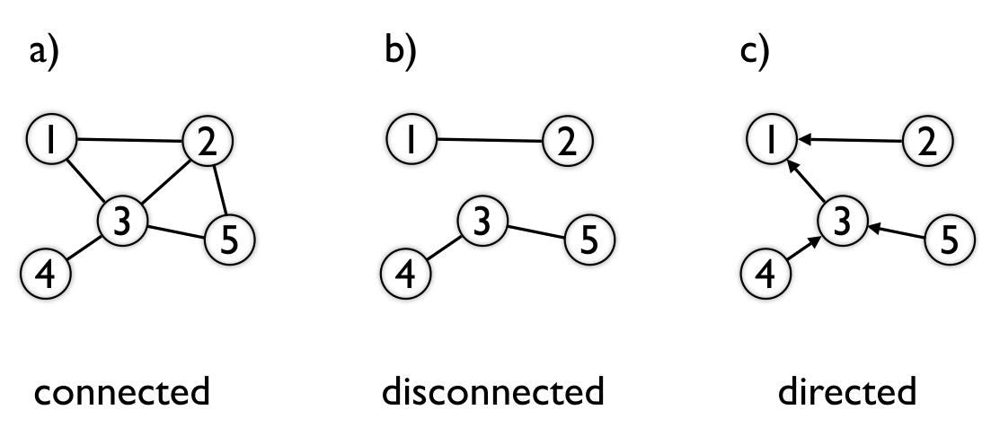
The network may be described in terms of its adjacency matrix A, which encodes the topological information, and is defined as

$$A_{ij}=\left\{\begin{array}[]{cc}1&\mbox{if }i\mbox{ and }j\mbox{ are connected}\\ 0&\mbox{ otherwise }.\end{array}\right.$$

An undirected graph has a symmetric adjacency matrix. The degree $k_{i}$ of the $i$th node is the number of connections it receives, clearly

$$k_{i}=\sum_{j=1}^{n}A_{ij}.$$

Another important matrix associated with the network is the combinatorial Laplacian matrix L, defined as

$$L_{ij}=\left\{\begin{array}[]{cc}k_{i}&\mbox{ if }i=j\\ -1&\mbox{if }i\mbox{ and }j\mbox{ are connected}\\ 0&\mbox{ otherwise }.\end{array}\right.$$

The Laplacian L is closely related to the adjacency matrix A. In a compact form it reads

$$\textbf{L}=\textbf{D}-\textbf{A},$$

where $\textbf{D}=$ diag$(k_{1},\cdots,k_{n})$ is the matrix of degrees. We depict in Fig. 2 distinct networks of size $4$ and their adjacency and Laplacian matrices.

The eigenvalues and eigenvectors of A and L tell us a lot about the network structure. The eigenvalues of L for instance, are related to how well-connected the graph is and how fast a random walk on the graph could spread. In particular, the smallest nonzero eigenvalue of L will determine the synchronization properties of the network. Since the graph is undirected, the matrix L is symmetric, its eigenvalues are real, and L has a complete set of orthonormal eigenvectors 9. The next result characterizes important properties of the Laplacian

Proof : The statement $a)$ follows from the fact that L is symmetric $\textbf{L}=\textbf{L}^{*}$, see Ap. id1 Theorem 9. To prove $b)$ consider the $\textbf{1}=(1,1,\cdots,1)^{*}$ and note that

$$(\textbf{L 1})_{i}=\sum L_{ij}=k_{i}-\sum_{j}A_{ij}=0$$

(1)

Item $c)$ follows from the Gershgorin theorem, see Ap. id1 Theorem 8. The nontrivial conclusion $d)$ is one of the main properties of the spectrum. To prove the statement $d)$ we first note that if the graph $G$ has $r$ connected components $G_{1},\cdots,G_{r}$, then is possible to represent L such that it splits into blocks $\textbf{L}_{1},\cdots,\textbf{L}_{r}$.

Let $m$ denote the multiplicity of $0$. Then Each $\textbf{L}_{i}$ has an eigenvector $\textbf{z}_{i}$ with $0$ as an eigenvalue. Note that $\textbf{z}_{i}=(z_{i}^{1},\cdots z_{i}^{n})$ can be defined as $z_{i}^{j}$ is equal to 1 if $j$ belongs to the component $i$ and zero otherwise, hence $m\geq r$. It remains to show that any eigenvector g associated with $0$ is also constant. Assume that g is a non-constant eigenvector associated with $0$, and let $g_{\ell}>0$ be the largest entry of g. Then

	$\displaystyle(\textbf{L g})_{\ell}$	$\displaystyle=$	$\displaystyle\sum_{j}L_{\ell j}g_{j}$
		$\displaystyle=$	$\displaystyle\sum_{j}(k_{\ell}\delta_{\ell j}-A_{\ell j})g_{j},$

since g is associated with the $0$ eigenvalue we have

$$g_{\ell}=\frac{\sum_{j}A_{\ell j}g_{j}}{k_{\ell}}.$$

This means that the value of the component $g_{\ell}$ is equal to the average of the values assigned to its neighbors. Hence g must be constant, which completes the proof. $\Box$

Therefore, $\lambda_{2}$ is bounded away from zero whenever the network is connected. The smallest non-zero eigenvalue is known as algebraic connectivity, and it is often called the Fiedler value. The spectrum of the Laplacian is also related to some other topological invariants. One of the most interesting connections is its relation to the diameter, size, and degrees.

We will not present the proof of the Theorem here, however, it can be found in the references we provide in the theorem. We suggest the reader see further bounds on the spectrum of the Laplacian in Ref. [50]. Also, Ref. [51] presents many applications of the Laplacian eigenvalues to diverse problems. One of the main goals in spectral graph theory is the obtain better bounds by having access to further information on the graphs.

For a fixed network size, the magnitude of $\lambda_{2}$ reflects how well-connected the graph is. Although the bounds given by Theorem 2 are general, they can be tight for certain graphs. For the ring, the lower bound on $\lambda_{2}$ is tight. This implies that as the size increases – consequently also its diameter – $\lambda_{2}$ converges to zero, and the network becomes effectively disconnected. In sharp contrast, we find the star network. In this case, the upper bound in $i)$ is tight. The star diameter is equal to two, regardless of the size, and $\lambda_{2}=1$. See the table for the precise values.

The networks we encounter in real applications have a wilder connection structure. Typical examples are cortical networks, the Internet, power grids, and metabolic networks [1]. These networks don’t have a regular structure of connections, such as the ones presented in Fig. 2. We say that the network is complex if it does not possess a regular connectivity structure.

One of the goals is to understand the relation between the topological organization of the network and its functional relation, such as its collective motion. In Fig. 3, we depict two networks used to model real networks, namely the Barabasi-Albert and the Erdos-Renyi Networks.

The Erdös-Rényi network is generated by setting an edge between each pair of nodes with equal probability $p$, independently of the other edges. If $p\gg\ln n/n$, then the network is almost surely connected, that is, as $N$ tends to infinity, the probability that a graph on $n$ vertices is connected tends to $1$. The degree is pretty homogeneous; almost surely every node has the same expected degree [34].

The Barabasi-Albert network possesses a great deal of heterogeneity in the nodes’ degrees, while most nodes have only a few connections, some nodes, termed hubs, have many connections. These networks do not arise by chance alone. The network is generated by means of the cumulative advantage principle – the rich get richer. According to this process, a node with many links will have a higher probability of establishing new connections than a regular node. The number of nodes of degree $k$ is proportional to $k^{-\beta}$. These networks are called scale-free networks [1]. Many graphs arising in various real-world networks display a similar structure to the Barabasi-Albert network [2, 3].

\motto

How can intuition deceive us at this point ?
          – Henri Poincaré

We say that set $\Omega\subset\mathbb{R}^{m}$ under the dynamics of Eq. (2) is positively invariant if the trajectories starting at the set never leave it in the future, that is, if $\textbf{x}(t_{0})\in\Omega$ then $\textbf{x}(t)\in\Omega$ for all $t\geq t_{0}$ Intuitively, it means that once the trajectory enters $\Omega$ it never leaves it again. The system is called dissipative if the solutions enter a positively invariant set $\Omega\subset D$ in finite time. $\Omega$ is called the absorbing domain of the system. The existence of an absorbing domain guarantees that the solutions are bounded, hence, the extension results in Ap. id1 Theorem 17 assures the global existence of the solutions.

The question is then how to obtain the absorbing domains. Note that whenever f is nonlinear, finding the solutions of Eq. 2 can be a rather intricate problem. And usually we won’t be able to do it analytically. So we need new machinery to address the problem on absorbing domains. A method by Lyapunov allows us to obtain such domains without finding the trajectories. The technique infers the existence of the absorbing domains in relation to some properties of a scalar function – the Lyapunov function.

We will study notions relative to connected nonempty subsets $\Omega$ of $\mathbb{R}^{m}$. A function $V:\mathbb{R}^{m}\rightarrow\mathbb{R}$ is said to be positive definite with respect to the set $B$ if $V(\textbf{x})>0$ for all $\textbf{x}\in\mathbb{R}^{q}\backslash\Omega$. It is radially unbounded if

$$\lim_{\|\textbf{x}\|\rightarrow\infty}V(\textbf{x})=\infty.$$

Note that this condition guarantees that all level sets of $V$ are bounded. This fact plays a central role in the analysis. We also define $V^{\prime}:\mathbb{R}^{m}\rightarrow\mathbb{R}$ as

$$V^{\prime}(\textbf{x})=\nabla V(\textbf{x})\cdot\textbf{f}(\textbf{x}).$$

where $\cdot$ denotes the Euclidean inner product. This definition agrees with the time derivative along the trajectories. That is, if $\textbf{x}(t)$ is a solution of Eq. (2), then by the chain rule we have

$$\frac{dV(\textbf{x}(t))}{dt}=V^{\prime}(\textbf{x}(t)).$$

The main result is then the following

Proof: Note that for any trajectory $\textbf{x}(t)$ in virtue of the fundamental theorem of the calculus

$$V(\textbf{x}(t))-V(\textbf{x}(s))=\int_{s}^{t}V^{\prime}(\textbf{x}(u))du<0.$$

So $V(\textbf{x}(t))<V(\textbf{x}(s))$ for any $t>s$, and $V$ is decreasing along solutions and is radially unbounded, the level sets

$$S_{a}=\{\textbf{x}\in\mathbb{R}^{m}:V(\textbf{x})\leq a\}$$

are positively invariant. Hence, the solutions are bounded, and will lie in smaller level sets as time increases until the trajectory enters $\Omega$. It remains to show that once the solutions lie in $\Omega$, they don’t leave it.

Suppose $\textbf{x}(t)$ leaves $\Omega$ at $t_{0}$ and let $b=V(\textbf{x}(t_{0}))$. The level set $S_{b}$ is closed, and there is a ball $B_{r}(\textbf{x}(t_{0}))$ such that $\textbf{x}(t_{0}+\varepsilon)\in B_{r}(\textbf{x}(t_{0}))\backslash S_{b}$ for some small $\varepsilon$. Hence, $V(\textbf{x}(t_{0}+\varepsilon))>V(\textbf{x}(t_{0}))$ contradicting the fact that $V$ is decreasing along solutions. $\Box$

There are also converse Lyapunov theorems [52]. Typically, if the system is dissipative (and has nice properties), then there exists a Lyapunov function. Although the above theorem is very useful, since we don’t need knowledge of the trajectories, the drawback is the function $V$ itself. There is no recipe to obtain a function $V$ fulfilling all these properties. One could always try to guess the function, or go for a general form such as choosing a quadratic function $V$. We assume that the Lyapunov function is given.

$$V(\textbf{x})=\frac{1}{2}(\textbf{x}-\textbf{a})^{*}\textbf{Q}(\textbf{x}-\textbf{a}).$$

where $\textbf{a}\in\mathbb{R}^{m}$. Consider the set $\Omega:=\{\textbf{x}\in\mathbb{R}^{m}\,\,|\,\,(\textbf{x}-\textbf{a})^{\dagger}\textbf{Q}(\textbf{x}-\textbf{a})\leq\rho^{2}\}$, then

$$V^{\prime}(\textbf{x})<0\ ,\forall\textbf{x}\in\mathbb{R}^{m}\backslash\Omega.$$

Under Assumption 1, Theorem 3 guarantees that $\Omega$ is positively invariant and that the trajectories of Eq. (2) eventually enter it. So, $\Omega$ is the absorbing domain of the problem. The solutions are, therefore, globally defined.

Since the system Eq. (2) is dissipative, the solutions accumulate in a neighborhood of a bounded set $\Lambda\subset\Omega$. The set $\Lambda$ is called an attractor. We focus on the situation where $\Lambda$ is a chaotic attractor. Now, the definition of a chaotic attractor is rather intricate – there is even a general definition, the important properties for us are that solutions on the attractor are aperiodic, i.e., there is no $\tau\geq 0$ such that $\textbf{x}(t)=\textbf{x}(t+\tau)$, and the solutions exhibits sensitive dependence on initial conditions. Sensitive dependence on initial conditions means that nearby trajectories separate exponentially fast.

If the system is chaotic, no matter how close two solutions start, they move apart when they are close to the attractor. Hence, arbitrarily small modifications of initial conditions typically lead to quite different states for large times. This sensitive dependence on initial conditions is one of the main features of a chaotic system. Exponential divergence cannot go on forever, since the attractor is bounded, it is possible to show that the trajectories will come close together in the future [53].

We introduce now the network model. On top of each node of the network, we introduce a copy of the system Eq. (2). Then the influence that the neighbor $j$ exerts on the dynamics of the node $i$ will be proportional to the difference of their state vector $\textbf{x}_{j}(t)-\textbf{x}_{i}(t)$. This type of coupling is called diffusive – it tries to equate to state of the nodes.

We label the nodes according to their degrees $k_{n}\geq\cdots\geq k_{2}\geq k_{1}$, where $k_{1}$ and $k_{n}$ denote the minimal and maximal degree, respectively. The dynamics of a network of $n$ identically diffusively coupled elements is described by

$\displaystyle\frac{d\textbf{x}_{i}}{dt}$

$\displaystyle=$

$\displaystyle\textbf{f}(\textbf{x}_{i})+\alpha\sum_{j=1}^{n}A_{ij}(\textbf{x}_{j}-\textbf{x}_{i}),$

(3)

where $\alpha$ is the overall coupling strength. In Eq. (3) the coupling is given in terms of the adjacency matrix. We can also represent the coupled equations in terms of the network Laplacian. Consider the coupling term

	$\displaystyle\sum_{j=1}^{n}A_{ij}(\textbf{x}_{j}-\textbf{x}_{i})$	$\displaystyle=$	$\displaystyle\sum_{j=1}^{n}A_{ij}\textbf{x}_{j}-k_{i}\textbf{x}_{i}$
		$\displaystyle=$	$\displaystyle\sum_{j=1}^{n}(A_{ij}-\delta_{ij}k_{i})\textbf{x}_{j}$

where $\delta_{ij}$ is the Kronecker delta, and recalling that $L_{ij}=\delta_{ij}k_{i}-A_{ij}$ we obtain Hence, the equations read

$\displaystyle\frac{d\textbf{x}_{i}}{dt}$

$\displaystyle=$

$\displaystyle\textbf{f}(\textbf{x}_{i})-\alpha\sum_{j=1}^{n}L_{ij}\textbf{x}_{j}.$

(4)

The dynamics of such a diffusive model can be intricate. Indeed, even if the isolated dynamics possesses a globally stable fixed point, the diffusive coupling can lead to the instability of the fixed points, and the systems can exhibit an oscillatory behavior. Please, see [56] for a discussion and further material. We will not focus on such a scenario of instability, but rather on how the diffusive coupling can lead to synchronization.

Note that due to the diffusive nature of the coupling, if all oscillators start with the same initial condition, the coupling term vanishes identically. This ensures that the globally synchronized state

$$\textbf{x}_{1}(t)=\textbf{x}_{2}(t)=\cdots=\textbf{x}_{n}(t)=\textbf{s}(t),$$

is an invariant state for all coupling strengths $\alpha$. The question is then the stability of synchronized solutions, which takes place due to coupling. Note that, if $\alpha=0$ the oscillators are decoupled, and Eq. (4) describes $n$ copies of the same oscillator with distinct initial conditions. Since the chaotic behavior leads to a divergence of nearby trajectories, without coupling, any small perturbation on the globally synchronized motion will grow exponentially fast, and lead to distinct behavior between the node dynamics.

The correct way to see the invariant of globally synchronized motion is as follows. First consider

$$\textbf{X}=\mbox{col}(\textbf{x}_{1},\cdots,\textbf{x}_{n}),$$

where col denotes the vectorization formed by stacking the column vectors $\textbf{x}_{i}$ into a single column vector. Similarly

$$\textbf{F}(\textbf{X})=\mbox{col}(\textbf{f}(\textbf{x}_{1}),\cdots,\textbf{f}(\textbf{x}_{n})),$$

then Eq. (4) can be arranged into a compact form

$$\frac{d\textbf{X}}{dt}=\textbf{F}(\textbf{X})-\alpha(\textbf{L}\otimes\textbf{I}_{m})\textbf{X}$$

(5)

where $\otimes$ is the Kronecker product, see Appendix id1. Let ${\Phi}(\cdot,t)$ be the flow of Eq. (5), the solution of the equation with initial condition $\textbf{X}_{0}$ is given by $\textbf{X}(t)={\Phi}(\textbf{X}_{0},t)$. Consider the synchronization manifold

$$\mathcal{M}=\{\textbf{x}_{i}\in\mathbb{R}^{m}:\textbf{x}_{i}(t)=\textbf{s}(t)\mbox{ for }1\leq i\leq n\},$$

then we have the following result

Proof: Recall that $\textbf{1}\in\mathbb{R}^{n}$ is such that every component is equal to $1$. Let $\textbf{X}(t)=\textbf{1}\otimes\textbf{s}(t)$, note that

$$\frac{d\textbf{X}(t)}{dt}=\textbf{1}\otimes\frac{d\textbf{s}(t)}{dt}.$$

We claim that $\textbf{X}(t)$ is a solution of the equations of motion.

	$\displaystyle\frac{d\textbf{X}(t)}{dt}$	$\displaystyle=$	$\displaystyle\textbf{F}(\textbf{X}(t))-\alpha(\textbf{L}\otimes\textbf{I}_{m})\textbf{X}(t)$
		$\displaystyle=$	$\displaystyle\textbf{F}(\textbf{1}\otimes\textbf{s}(t))-\alpha(\textbf{L}\otimes\textbf{I}_{m})\textbf{1}\otimes\textbf{s}(t)$
		$\displaystyle=$	$\displaystyle\textbf{1}\otimes\textbf{f}(\textbf{s}(t))$

where in the last passage we used Theorem () together with L 1 = 0 and $\textbf{F}(\textbf{1}\otimes\textbf{s}(t))=\textbf{1}\otimes\textbf{f}(\textbf{s}(t))$. By the Picard-Lindelöf Theorem 16 we have that that $\textbf{X}(t)={\Phi}(\textbf{1}\otimes\textbf{s}(0),t)\in\mathcal{M}$ for all $t$. $\Box$

If the oscillators have the same initial condition, their evolution will be exactly the same forward in time, no matter the value of the coupling strength.

In the above result, we have looked at the network not as a coupled equation but as a single system in the full state space $\mathbb{R}^{mn}$. We prefer to keep the picture of coupled oscillators. These pictures are equivalent, and we interchange them whenever it suits our purposes. The important questions are

•

Boundedness of the solutions $\textbf{x}_{i}(t)$.

•

Stability of the globally synchronized state (synchronization manifold).

We wish to address the local stability of the globally synchronized state. That is, if all trajectories start close together $\|\textbf{x}_{i}(0)-\textbf{x}_{j}(0)\|\leq\varepsilon$, for any $i$ and $j$ and some small $\varepsilon$, would they converge to $\mathcal{M}$, in other words, would

$$\lim_{t\rightarrow\infty}\|\textbf{x}_{i}(t)-\textbf{x}_{j}(t)\|=0$$

or would the trajectories split apart? The goal of the remaining exposition is to provide positive answers to these questions. To this end, we review some fundamental results needed to address such points.

\motto

The more you know, the less sure you are.
          – Voltaire

Let $\textbf{y}(0)$ be close to $\textbf{s}(0)$. Each of these distinct points has its behavior determined by the equation of motion Eq. (2). We can follow the dynamics of the difference

$$\textbf{z}(t)=\textbf{y}(t)-\textbf{s}(t)$$

which leads to the variational equations governing its evolution

	$\displaystyle\frac{d\textbf{z}(t)}{dt}$	$\displaystyle=$	$\displaystyle\textbf{f}(\textbf{y}(t))-\textbf{f}(\textbf{s}(t))$
		$\displaystyle=$	$\displaystyle\textbf{f}(\textbf{s}(t)+\textbf{z}(t))-\textbf{f}(\textbf{s}(t)),$

now since $\|\textbf{z}\|$ is sufficiently small we may expand the function f in Taylor series

$$\textbf{f}(\textbf{s}(t)+\textbf{z}(t))=\textbf{f}(\textbf{s}(t))+D\textbf{f}(\textbf{s}(t))\textbf{z}(t)+\textbf{R}(\textbf{z}(t))$$

where $D\textbf{f}(\textbf{s}(t))$ along the trajectory $\textbf{s}(t)$, and by the Lagrange theorem [57]

$$\|\textbf{R}(\textbf{z}(t))\|=O(\|\textbf{z}(t)\|^{2}).$$

Truncating the evolution equation of z, up to the first order, we obtain the first variational equation

$\displaystyle\frac{d\textbf{z}}{dt}=D\textbf{f}(\textbf{s}(t))\textbf{z}.$

Note that the above equation is non-autonomous and linear. Moreover, since $\textbf{s}(t)$ lies in a compact set and f is continuously differentiable, by Weierstrass Theorem [57], $D\textbf{f}(\textbf{s}(t))$ is a bounded matrix function. If $\|\textbf{z}(t)\|\rightarrow 0$ the two distinct solutions converge to each other and have an identical evolution.

The first variational equation plays a fundamental role to tackling the local stability problem. Suppose that somehow we have succeeded to demonstrate that the trivial solution of the first variational equation is stable. Note that this does not completely solve our problem, because the Taylor remainder acts as a perturbation of the trivial solution. Hence, to guarantee that the problem can be solved in terms of the variational equation we must also obtain conditions on the persistence of the stability of trivial solution under small perturbation. There is a beautiful and simple, yet general, criterion based on uniform contractions. We follow closely the exposition in Ref. [58, 59].

Consider the linear differential equation

$$\frac{d\textbf{x}}{dt}=\textbf{U}(t)\textbf{x}$$

(6)

where $\textbf{U}(t)$ is a continuous bounded linear operator on $\mathbb{R}^{q}$ for each $t\geq 0$.

The point $\textbf{x}\equiv\textbf{0}$ is an equilibrium point of the equation Eq. (6). Loosely speaking, we say an equilibrium point is locally stable if the initial conditions are in a neighborhood of zero solution remain close to it for all time. The zero solution is said to be locally asymptotically stable if it is locally stable and, furthermore, all solutions starting near 0 tend towards it as $t\rightarrow\infty$.

The time dependence in Eq. (6) introduces of additional subtleties [60]. Therefore, we want to state some precise definitions of stability

Lyapunov stability is a very mild requirement on equilibrium points. In particular, it does not require that trajectories starting close to the origin tend to the origin asymptotically. Also, stability is defined at a time instant $t_{0}$. Uniform stability is a concept which guarantees that the equilibrium point is not losing stability. We insist that for a uniformly stable equilibrium point $\textbf{x}^{*}$, $\delta$ in the Definition 4.1 not be a function of $t_{0}$, so that equation may hold for all $t_{0}$. Asymptotic stability is made precise in the following definition:

We shall focus on the concept of uniform asymptotic stability. To this end, we wish to express the solutions of the linear equation in a closed form. The theory of differential equations guarantees that the unique solution of the above equation can be written in the form

$$\textbf{x}(t)=\textbf{T}(t,s)\textbf{x}(s)$$

where $\textbf{T}(t,s)$ is the associated evolution operator [59]. The evolution operator satisfies the following properties

	$\displaystyle\textbf{T}(t,s)\textbf{T}(s,u)$	$\displaystyle=$	$\displaystyle\textbf{T}(t,u)$
	$\displaystyle\textbf{T}(t,s)\textbf{T}(s,t)$	$\displaystyle=$	$\displaystyle\textbf{I}_{m}.$

The following concept plays a major role in these lectures

Some examples of evolution operators and uniform contractions are

We will show that the trivial solution of Eq. 6 is uniformly asymptotically stable if, and only if, the evolution operator is a uniform contraction, that is, the solutions converge converges exponentially fast to zero.

Proof: First suppose the evolution operator is a uniform contraction then

	$\displaystyle\|\textbf{x}(t)\|$	$\displaystyle=$	$\displaystyle\|\textbf{T}(t,s)\textbf{x}(s)\|$
		$\displaystyle\leq$	$\displaystyle\|\textbf{T}(t,s)\|\|\textbf{x}(s)\|$
		$\displaystyle\leq$	$\displaystyle Ke^{-\alpha(t-s)}\|\textbf{x}(s)\|.$

Now let $\varepsilon>0$ be given, clearly if $t>T$, where $T=T(\varepsilon)$ is large enough then the $\|\textbf{x}(t)\|\leq\varepsilon.$ Let $\|\textbf{x}(s)\|\leq\delta$, we obtain $\|\textbf{x}(t)\|\leq Ke^{-\alpha(t-s)}\delta<\varepsilon,$ which implies that

$$T=T(\varepsilon)=\frac{1}{\alpha}\ln\frac{\delta K}{\varepsilon},$$

completing the first part.

To prove the converse, we assume that the trivial solution is uniformly asymptotically stable. Then there is $\delta$ such that for any $\varepsilon$ and $T=T(\varepsilon)$ such that for any $\|\textbf{x}(s)\|\leq\delta$ we have

$$\|\textbf{x}(t)\|\leq\varepsilon,$$

for any $t\geq s+T$. Now take $\varepsilon=\delta/k$, and consider the sequence $t_{n}=s+nT$.

Note that

$$\|\textbf{T}(t,s)\textbf{x}(s)\|\leq\frac{\delta}{k},$$

for any $\|\textbf{x}(s)\|/\delta\leq 1$, we have the following bound for the norm

$$\|\textbf{T}(t,s)\|=\sup_{\|\textbf{u}\|\leq 1}\|\textbf{T}(t,s)\textbf{u}\|\leq\frac{1}{k}.$$

Remember that $\textbf{T}(t,u)\textbf{T}(u,s)=\textbf{T}(t,s)$. Hence,

	$\displaystyle\|\textbf{T}(t_{2},s)\|$	$\displaystyle=$	$\displaystyle\|\textbf{T}(s+2T,s+T)\textbf{T}(s+T,s)\|$
		$\displaystyle\leq$	$\displaystyle\|\textbf{T}(s+2T,s+T)\|\|\textbf{T}(s+T,s)\|$
		$\displaystyle\leq$	$\displaystyle\frac{1}{k^{2}}.$

Likewise, by induction

$$\|\textbf{T}(t_{n},s)\|\leq\frac{1}{k^{n}},$$

take $\alpha=\ln k/T$, therefore,

$$\|\textbf{T}(t_{n},s)\|\leq e^{-\alpha(t_{n}-s)}.$$

Consider the general case $t=s+u+nT$, where $0\leq u<T$, then the same bound holds

	$\displaystyle\|\textbf{T}(t,s)\|$	$\displaystyle\leq$	$\displaystyle e^{-nT\alpha}$
		$\displaystyle\leq$	$\displaystyle Ke^{-(t-s)\alpha},$

where $K\leq e^{\alpha T}$, and we conclude the desired result. $\Box$

The uniform contractions have a rather important roughness property, they are not destroyed under perturbations of the linear equations.

Proof: Let us start by noting that the evolution operator $\textbf{T}(t,s)$ also satisfies the differential equation of the unperturbed problem

$$\frac{d}{dt}\textbf{T}(t,s)=\textbf{U}(t)\textbf{T}(t,s),$$

The evolution operator $\hat{\textbf{T}}$ can be obtain by the variation of parameter, see Ap. id1 Theorem 18. So,

$$\hat{\textbf{T}}(t,s)=\textbf{T}(t,s)+\int_{s}^{t}\textbf{T}(t,u)\textbf{ V}(u)\hat{\textbf{T}}(u,s)du,$$

using the induce norm, for $t\geq s$,

$$\|\hat{\textbf{T}}(t,s)\|\leq Ke^{-\eta(t-s)}+\delta K\int_{s}^{t}e^{-\eta(t-u)}\|\hat{\textbf{T}}(u,s)\|du.$$

Let us introduce the scalar function $w(u)=e^{-\eta(t-u)}|\hat{\textbf{T}}(t,s)|$, then

$$w(t)\leq Kw(s)+K\delta\int_{s}^{t}w(u)du,$$

for all $t\geq s$. Now we can use the Gronwall’s inequality to estimate $w(t)$, see Ap. id1 Theorem 2, this implies

$$w(t)\leq Kw(s)e^{\delta K(t-s)},$$

consequently

$$\|\hat{\textbf{T}}(t,s)\|\leq Ke^{\left(\eta-K\delta\right)(t-s)}.$$

$\Box$

The roughness property of uniform contraction does the job and guarantees that the stability of the trivial solution is maintained. The question now turns to how to obtain a criterion for uniform contractions. There are various criteria, and the following suits our purposes

Proof: Note that we can write $\|\textbf{R}(\textbf{y})\|\leq K\|\textbf{y}\|^{1}$, where $K=M\|\textbf{y}\|$. Now given a neighborhood of the trivial solution $\|\textbf{y}\|\leq\delta$ is possible to control $K\leq\varepsilon$. Applying the previous Proposition 3 we conclude the result. $\Box$

This result can be used to prove that if the origin of a nonlinear system is uniformly asymptotically stable then the linearized system about the origin describes the behavior of the nonlinear system.

The question now concerns the criteria to obtain a uniform contraction. There are many results in this direction, we suggest Ref. [58]. We present a criterion that best suits our purpose. The criterion provides a condition only in terms of the equation, and requires no knowledge of the solutions.

Proof: We use the norm $\|\cdot\|_{\infty}$ and its induced norm, see Ex 4 in Ap. id1. Let $\textbf{ x}(t)$ be a solution. For a fixed time $u>0$ and let $\|\textbf{x}(u)\|_{\infty}^{2}=x_{i}(u)^{2}$. Note $\textbf{ x}(t)$ is a differentiable function and the norm a continuous function $x_{i}(t)^{2}$ will also be the norm in an open interval $I=(u-a,u+a)$ for some $a>0$. Therefore,

	$\displaystyle\frac{1}{2}\frac{d}{dt}\|\textbf{ x}(t)\|_{\infty}^{2}$	$\displaystyle=$	$\displaystyle\frac{1}{2}\frac{d}{dt}[x_{i}(t)]^{2}$
		$\displaystyle=$	$\displaystyle x_{i}(t)\left(\sum_{j=1}^{m}U_{ij}x_{j}\right)$
		$\displaystyle=$	$\displaystyle U_{ii}(t)x_{i}^{2}(t)+\sum_{j=1,\atop j\not=i}^{m}U_{ij}x_{i}(t)x_{j}(t)$
		$\displaystyle\leq$	$\displaystyle U_{ii}(t)x_{i}^{2}(t)+\sum_{j=1,\atop j\not=i}^{m}|U_{ij}(t)|x_{i}^{2}(t),$

and consequently,

$\displaystyle\frac{1}{2}\frac{d}{dt}\|\textbf{x}(t)\|_{\infty}^{2}\leq\left(U_{ii}(t)+\sum_{j=1,\atop j\not=i}^{m}|U_{ij}(t)|\right)\|\textbf{x}(t)\|_{\infty}^{2}.$

Using the condition

$$U_{ii}(t)+\sum_{j=1,\atop j\not=i}^{m}|U_{ij}(t)|\leq-\eta<0,$$

(8)

replacing in the inequality

$$\frac{1}{2}\frac{d}{dt}\|\textbf{x}(t)\|_{\infty}^{2}\leq-\eta\|\textbf{x}(t)\|_{\infty}^{2},$$

an integration yields

$$\|\textbf{x}(t)\|_{\infty}^{2}\leq\|\textbf{x}(s)\|_{\infty}^{2}-2\eta\int_{s}^{t}\|\textbf{x}(\tau)\|_{\infty}^{2}d\tau,$$

for all $t,s\in I$ and $t>s$. Applying the Gronwall inequality we have which implies

$$\|\textbf{x}(t)\|_{\infty}\leq e^{-\eta(t-s)}\|\textbf{x}(s)\|_{\infty}.$$

(9)

Next note that the argument does not depend on the particular component $i$, because we assume that Eq. (8) is satisfied for any $1\leq i\leq m$. So the norm will satisfy the bound in Eq. 9 for any compact set of $\mathbb{R}_{+}$. Noting that all norms are equivalent in finite dimensional spaces the result follows $\Box$.

References

- (1) M. E. J. Newman, Networks: An Introduction, Oxford University Press (2010).
- (2) R. Albert, H. Jeong, A.-L. Barabási A.-L. , Nature 406, 378 (2000).
- (3) R. Albert, A.-L. Barabási, Rev. Mod. Phys. 74, 47 (2002).
- (4) D.L. Turcotte, Fractals and Chaos in Geology and Geophysics, 2nd edn, Cambridge UP, 1997.
- (5) R.M. May, Stability and Complexity in Model Ecosystems, Princeton UP, 1973.
- (6) S.A. Levin, B.T. Grenfell, A. Hastings, A.S. Perelson, Science 275, 334–343 (1997).
- (7) E. Bullmore, O. Sporns, Nature Neurosc. 10, 186 (2009).
- (8) J. Pantaleone, Phys. Rev. D 58, 3002 (1998).
- (9) K. Wiesenfeld, P. Colet, and S. Strogatz, Phys. Rev. E 57, 1563 (1998).
- (10) A.T. Winfree, The Geometry of Biological Time, Springer, 1980.
- (11) Y. Kuramoto, Chemical Oscillations, Waves, and Turbulence, Springer, 1984.
- (12) P. Fries, Trends Cogn.Sci. 9, 474 (2005) .
- (13) T. Pereira, Phys. Rev. E 82, 036201 (2010).
- (14) T Stankovski, T Pereira, PVE McClintock, A Stefanovska, Reviews of Modern Physics 89, 045001 (2017)
- (15) S. Strogatz,Sync: The Emerging Science of Spontaneous Order, Hyperion, New York, (2003).
- (16) A. Arenas, A. Diaz-Guilera, J. Kurths, Y. Moreno, C. Zhou Synchronization in complex networks, Physics Rep. 469, 93 (2008).
- (17) C. W. Wu, Synchronization in complex networks of nonlinear dynamical systems, World Scientific Publishing Co. Pte. Ltd., Singapore (2007).
- (18) H. Nijmeijer and A. Rodríguez-Angeles, Synchronization of mechanical systems, World Scientific Publishing Co. Pte. Ltd., Singapore (2003).
- (19) T Pereira, MS Baptista, J Kurths, Phys. Rev. E 75, 026216 (2007).
- (20) T Pereira, MS Baptista, J Kurths, Physica D 216, 260 (2006).
- (21) D Eroglu, JSW Lamb, T Pereira, Contemporary Physics 58, 207-243 (2017).
- (22) C.M. Gray, W. Singer, Proc. Nat. Acad. Sci. USA 86, 1698 (1989).
- (23) G.G. Gregoriou, S.J. Gotts, H. Zhou, R. Desimone Science 324, 1207 (2009).
- (24) W. Singer, Neuron 24, 49 (1999).
- (25) John Milton and Peter Jung (Ed), Epilepsy as a Dynamic Disease, Springer, 2010.
- (26) D Eroglu, M Tanzi, S van Strien, T Pereira, Physical Review X 10, 021047 (2020)
- (27) P. Tass, M.G. Rosenblum, J.Weule, et al., Phys.Rev.Lett. 81, 3291 (1998).
- (28) D.J.D. Earn, S.A. Levin, P. Rohani, Science 290, 1360 (2000).
- (29) B.T. Grenfell et al., Nature 414, 716 (2001).
- (30) S Ruschel, T Pereira, S Yanchuk, LS Young, Journal of Mathematical Biology 79, 249-279 (2019)
- (31) LS Young, S Ruschel, S Yanchuk, T Pereira, Scientific Reports 9, 3505 (2019)
- (32) L.M. Pecora and T.L. Carrol, Phys. Rev. Lett. 80, 2109 (1998);
- (33) V Vlasov, Y Zou, T Pereira Physical Review E 92 (1), 012904 (2015)
- (34) F. R. K. Chung and L. Lu, Complex Graphs and Networks, American Mathematical Society (2006).
- (35) A. Barrat, M. Barthelemi, A. Vespegnani, Dynamical Processes on Complex Networks, Cambridge University Press (2008).
- (36) T Pereira, S van Strien, M Tanzi Journal of the European Mathematical Society 22, 2183–2252 (2020)
- (37) C Poignard, T Pereira, JP Pade, SIAM Journal on Applied Mathematics 78, 372-394 (2018)
- (38) C Poignard, JP Pade, T Pereira, Journal of Nonlinear Science 29 (5), 1919-1942 (2019)
- (39) M. Barahona and L.M. Pecora, Phys. Rev. Lett. 89, 054101 (2002).
- (40) A.E. Motter, C. Zhou, and J. Kurths, Phys. Rev. E 71, 016116 (2005).
- (41) J Eldering, JSW Lamb, T Pereira, ER dos Santos, Nonlinearity 34 (8), 5344 (2021)
- (42) RM Corder, Z Bian, T Pereira, A Montalbán, Chaos, 33, 091103 (2022)
- (43) Z Bian, JSW Lamb, T Pereira, Communications in Mathematical Physics 406, 170 (2025).
- (44) T. Pereira, D. Eroglu, G. B. Bagci, U. Tirnakli, H. J. Jensen, Phys. Rev. Lett. 110, 234103 (2013).
- (45) T. Pereira, J. Eldering, M. Rasmussen, A. Veneziani, Towards a general theory for coupling functions allowing persistent synchronization, Nonlinearity 27 (3), 501 (2014).
- (46) L. Barreira and Y.B. Pesin , Lyapunov Exponents and Smooth Ergodic Theory, American Mathematical Society (2002).
- (47) B. Bollobas, Modern Graph Theory, Springer (1998).
- (48) Bojan Mohar, GRAPHS AND COMBINATORICS Volume 7, Number 1, 53-64, DOI: 10.1007/BF01789463
- (49) M. Fiedler, Algebraic connectivity of graphs, Czech. Math. J. 23 (98) (1973) 298–305.
- (50) B. Mohar, Graph Theory, Comb. Appl. 2, 871 (1991).
- (51) B. Mohar, Graph Symmetry: Algebraic Methods and Applications, NATO ASI Series C vol. 497 (1997), pgs. 227–275.
- (52) A. Bacciotti and L. Rosier, Liapunov Functions and Stability in Control Theory, Springer-Verlag Berlin Heidelberg (2005).
- (53) A. Katok, B. Hasselblatt, Introduction to the Modern Theory of Dynamical Systems, Cambridge UP, 1996.
- (54) M. Viana, What’s new on Lorenz strange attractors? Math. Intelligencer, 22, 6 (2000).
- (55) C. Sparow, The Lorenz Equations: Bifurcations, Chaos, and Strange Attractors, Springer (1982)
- (56) A. Pogromsky, T. Glad, and H. Nijmeijer, Int. J. Bif. Chaos 9, 629 (1999).
- (57) R. Courant, D. Hilbert. Methods of Mathematical Physics. Vol 1. Interscience Publishers, Inc. New York, 1953.
- (58) W.A. Coppel, Dichotomies in Stability Theory, Springer-Verlag Berlin Heidelberg New York (1978).
- (59) P. J. Antsaklis and A. N. Michel, Linear Systems, Mcgraw-Hill College (1997)
- (60) M. Rasmussen, Attractivity and Bifurcation for Nonautonomous Dynamical Systems, Lecture Notes in Mathematics 1907, Springer (2007).
- (61) A. Pogromsky and H. Nijmeijer, IEEE Trans. Circ. Sys. - I 48, 152 (2001).
- (62) V. Belykh, I. Belykh and M. Hasler, Physica D 195, 159 (2004).
- (63) C-H. Li and S-Y Yang, J. London Math. Soc. (2011); doi:10.1112/jlms/jdq096.
- (64) K. Josic, Phys. Rev. Lett. 80, 3053 (1998).
- (65) K. Josic, Nonlinearity 13, 1321 (2000).
- (66) L. Barreira and C. Valls, Stability of Nonautonomous Differential Equations, Springer-Verlag Berlin Heidelberg (2008).
- (67) P. Lancaster and M. Tismenetsky , The Theory of Matrices, Academic Press; 2 edition (1985).
- (68) G. H. Golub, C. F. Van Loan, Matrix Computations, The Johns Hopkins University Press; 3rd edition (1996).
- (69) P. Hartman, Ordinary Differential Equations, John Wiley & Sons, Inc, NY (1964).
- (70) M. W. Kirsch, S. Smale, e R.L. Devaney, Differential Equations, Dynamical Systems and An Introduction to Chaos, Academic Press, San Diego (2004).
- (71) P. Hartman, Ordinary Differential Equations, John Wiley & Sons, Inc, NY (1964).
- (72) E Nijholt, JL Ocampo-Espindola, D Eroglu, IZ Kiss, T Pereira, Nature communications 13 (1), 4849 (2022)
- (73) S Von Der Gracht, E Nijholt, B Rink, SIAM Journal on Applied Mathematics 83 (6), 2329-2353 (2023)
- (74) C Bick, E Gross, HA Harrington, MT Schaub SIAM review 65 (3), 686-731
- (75) R Tönjes, CE Fiore, T Pereira, Nature Communications 12 (1), 72 (2021)
- (76) JP Pade, T Pereira, Scientific Reports 5 (1), 9968 (2015)
- (77) JD Hart, JP Pade, T Pereira, TE Murphy, R Roy, Physical Review E 92 (2), 022804 (2015).