A New Method to Quantify X-ray Substructures in
Clusters of Galaxies

Felipe Andrade-Santos, Gastão B. Lima Neto, Tatiana Ferraz Laganá Affiliation: Universidade de São Paulo, Departamento de Astronomia, Instituto de
Astronomia, Geofísica e Ciências Atmosféricas, Rua do Matão 1226,
Cidade Universitária, 05508-090, São Paulo, SP, Brazil

Abstract

We present a new method to quantify substructures in clusters of galaxies, based on the analysis of the intensity of structures. This analysis is done in a residual image that is the result of the subtraction of a surface brightness model, obtained by fitting a two-dimensional analytical model ( $\beta$ -model or Sérsic profile) with elliptical symmetry, from the X-ray image. Our method is applied to 34 clusters observed by the Chandra Space Telescope that are in the redshift range $z\in[0.02,0.2]$ and have a signal-to-noise ratio greater than 100. We present the calibration of the method and the relations between the substructure level with physical quantities, such as the mass, X-ray luminosity, temperature, and cluster redshift. We use our method to separate the clusters in two sub-samples of high and low substructure levels. We conclude, using Monte Carlo simulations, that the method recuperates very well the true amount of substructure for small angular core radii clusters (with respect to the whole image size) and good signal-to-noise observations. We find no evidence of correlation between the substructure level and physical properties of the clusters such as mass, gas temperature, X-ray luminosity and redshift. The scaling relations for the two sub-samples (high and low substructure level clusters) are different (they present an off-set, i.e., given a fixed mass or temperature, low substructure clusters tend to be more X-ray luminous), which is an important result for cosmological tests using the mass-luminosity relation to obtain the cluster mass function, since they rely on the assumption that clusters do not present different scaling relations according to their dynamical state.

Keywords:

galaxies:clusters:general — large-scale structure of universe — X-ray:galaxy clusters

I Introduction

Clusters of galaxies are the largest virialized objects in the Universe, the upper limit of collapsed halo mass function. In an Universe dominated by a cosmological constant and cold dark matter ( $\Lambda$ CDM), dark matter halos are formed by gravitational instability from primordial quantum fluctuations in the mass density field. The amplitude of those fluctuations increases as they cease expanding with the Hubble flux, collapse and virialize, forming dense and relaxed structures. Smaller structures grow to larger ones through mergers, up to clusters of galaxies in the present time. In this hierarchical scenario of structures formation, clusters are thus dynamically young objects and contain evidence of their recent past merging history [19, e.g.]. We can relate substructures with the cluster dynamical age [30, 33, e.g.]: the more substructure (their total intensity) a cluster presents, the younger (dynamically speaking) it is.

The hot intra-cluster plasma is a powerful X-ray source and its observation reveals the projected spatial distribution of most of the baryonic mass. X-ray studies of galaxy clusters are thus particularly relevant in this context, as they can give us clues to the dynamical age of clusters (e.g., Henriksen et al. [10] – Abell 3266, Lima Neto et al. [22] – Abell 970, Ferrari et al. [9] – Abell 3921). Analysis of substructure in the intra-cluster plasma spatial distribution should help us determining the dynamical state of galaxy clusters. A very good review about the theory and observational status of the study of substructures based on X-ray data in clusters of galaxies is given by Jeltema et al. [14]. Here, we only briefly discuss some of the previous work on cluster substructures.

Jones & Forman [17] made the first X-ray systematic study of structures in galaxy clusters, visually analyzing 208 objects observed by the Einstein satellite, establishing that merging must be a common phenomenon in clusters. Richstone et al. [30] developed in an original theoretical study a relation between substructures and cosmology, where they put constraints on cosmological parameters by the fractional rate of major mergers in clusters.

X-ray surface brightness allows us to perform statistical tests such as centroid and ellipticity variation [25], relating the dynamical age of clusters with its morphology. Buote & Tsai [2], Buote & Tsai [3] developed a method to quantify X-ray substructures in clusters of galaxies from the moments of the expansion in Fourier series of the X-ray surface brightness. Jeltema et al. [14] used the same method, referred to as the power-ratio method, in a sample of 40 clusters of galaxies observed by Chandra. They showed that clusters in general are less relaxed at $z>0.5$ , than at $z\simeq 0$ .

Semi-analytic methods give an indication of the expected evolution of cluster substructure and its dependence on cosmological parameters, however, the best method of constraining cosmological models is probably through the comparison with hydrodynamic cluster simulations. For instance, Suwa et al. [33] compared simulated clusters in a $\Lambda$ CDM and an OCDM cosmology, at both $z=0$ and $z=0.5$ , using several methods for quantifying structure. They restrict themselves to comparing the ability of different statistical indicators in distinguishing different simulated cosmologies, showing that cluster structure can potentially constrain $\Omega_{\Lambda}$ or the dark energy equation of state.

Although a lot of effort has been done in order to advance our understanding about substructure in clusters of galaxies, from theoretical to numerical simulation studies, we propose in the present work a novel method of quantifying substructures that has a simple physical interpretation: the substructure level, the way it is defined, reflects the fraction of the total X-ray luminosity that is emitted by the substructures, serving as a tool to understand the underlying physical processes taking place during the cluster evolution.

This paper is organized as follows. In section 2, we describe the sample selection and in section 3 the data reduction and analysis are discussed. In section 4, the substructure level is defined and our method is described, with its calibrations being discussed in section 5. In section 6 the results are presented and discussed and conclusions are finally presented in section 7. The cosmology assumed in this paper is given by $\Omega_{M}=0.3$ , $\Omega_{\Lambda}=0.7$ and $H_{0}=70$ km s^-1Mpc^-1.

II Sample Definition

Our method was applied to 34 clusters observed by the Chandra X-ray Telescope ACIS-I detector, with signal-to-noise ratios ( $S/N$ ) greater than 100, and that are in the redshift range $z\in[0.02,0.2]$ . Figure 1 shows the cluster redshift distribution. There is an apparent gap within $z\in[0.12,0.14]$ . This is due to the incompleteness of the sample, but there is no particular redshift interval with an excess of objects and our results do not depend on the sample completeness.

The criteria for clusters selection were chosen so as to ensure a suitable signal-to-noise ratio and a large enough image to work upon, without introducing bias for specific clusters. However, biases that we do not control may affect our sample. Clusters are observed in time-competitive telescopes, so they must present something “special”, many times substructures and irregularities, that make them “worth” being observed. Therefore one should keep in mind this caveat, that it is possible that our sample may have a tendency to present more substructures than the average expected for all clusters in the redshift range $z\in[0.02,0.2]$ .

Refer to caption — Figure 1: Histogram of the redshift distribution of clusters in our sample.

III Data Reduction and Analysis

In order to obtain calibrated images without artifacts, adequate to be used with our method of substructure detection, it is necessary to follow a series of procedures of cleaning and filtering the X-ray data. Otherwise, we would have contamination that would be detected as spurious substructures.

III.1 Data Reduction

We have used the package CIAO 3.4. Initially a level 2 events file has been generated from a level 1 events file, using the standard pipeline procedure¹¹ 1 http://cxc.harvard.edu/ciao3.4/threads/createL2/ and the calibration files, CALDB 3.3.0. Periods with high particle background (flares) were excluded using the lc $\_$ clean script. At this point, a re-binned image with pixels corresponding to 16 raw physical pixels (4x4, which roughly corresponds to 2” pixels) is created from the new level 2 event file, in the energy band 0.3 to 7.0 keV. Then, we produce exposure maps and use them to obtain flat images from which the source points are removed by filling circles around each source with a random Poisson sampling with the same distribution as found in a circular region close to the source. Finally, we fit a 2D analytical surface brightness model.

III.2 Surface Brightness

The surface brightness profile is the projection of the plasma emissivity along the line of sight. We will assume two radial analytical profiles for the surface brightness: the $\beta$ -model [4] and the Sérsic [27, 7].

In order to take into account the ellipticity of the plasma emission we use the following standard coordinates transformation:

\left\{\begin{array}[]{l}x^{\prime}=(x-x_{0})\cos\theta-(y-y_{0})\sin\theta;\\ y^{\prime}=(x-x_{0})\sin\theta+(y-y_{0})\cos\theta;\\ r^{2}=x^{\prime 2}+\displaystyle\frac{y^{\prime 2}}{(1-\epsilon)^{2}},\\ \end{array}\right.

where $(x_{0},y_{0})$ is the X-ray emission center coordinates, $\theta$ is the position angle, and $\epsilon$ is the ellipticity.

The $\beta$ -model may now be defined as follows:

\Sigma(r)=\Sigma_{0}\left[1+\left(\frac{r}{r_{c}}\right)^{2}\right]^{-3\beta+0.5}+b,

where $r_{c}$ is the core radius, $\beta$ is the shape parameter, and $\Sigma_{0}$ is the central surface brightness. The parameter $b$ corresponds to the background, and is supposed to be constant throughout the image (hence the importance of the exposure map correction).

The Sérsic model is defined as follows:

\displaystyle\Sigma(r)=\Sigma_{0}\exp\left[-\left(\frac{r}{a}\right)^{\nu}\right]+b,

where $a$ is the scale parameter, $\nu$ (often represented as $1/n$ ) is the shape parameter and $b$ is again the background surface brightness.

Once we have the image correctly processed, we fit a 2D surface brightness model to it using a standard minimum squares method, $\chi^{2}$ , and obtain the residual image, which is going to be the starting point for substructure quantification.

We fitted the $\beta$ and Sérsic models for most of the clusters, and in the case where both models were fitted, we chose to use the one that gave the smaller substructure level (see below how the substructure level is defined and computed). In practical terms, this is the same as choosing the fit with the smallest $\chi^{2}$ . The 2D surface brightness model fitted for each cluster is presented in Table 2.

IV X-ray Substructures

Previous studies on ICM substructure have been done, either qualitatively [16, 17, 20, 21] or quantitatively [30, 2, 14], based on different techniques. There is, however, no method that takes into account the ratio between the number of counts on the residual and on the original images, which will be referred to as the residual flux method. We describe here this method to quantify the substructure on the intra-cluster plasma emission.

IV.1 Substructure Level

We start by defining a threshold for the residual image in order to identify the pixels which had a number of counts statistically significant above or below (positive and negative residues) the 2D surface brightness fitted model at the pixel position. The threshold in each pixel was defined as the square root of the number of counts of the model in the correspondent pixel, i.e., the expected variance.

Then we quantify the substructure level by computing the ratio between the total number of counts of the residual and original images (taking the absolute value of the negative counts in the residual image and treating them exactly as the counts in the positive regions - after selecting those (in absolute value) above the threshold). By construction, the substructure level, $S$ , is defined as:

\displaystyle S\equiv\frac{\displaystyle\sum_{i=1}^{n}\left|C_{i}^{r}\right|}{\displaystyle\sum_{i=1}^{n}C_{i}^{t}},

(1)

where $C_{i}^{r}$ is the number of counts of the $i$ -th residual image pixel and $C_{i}^{t}$ is the number of counts of the $i$ -th image pixel and $n$ is the number of pixels of the image.

We defined the substructure level this way because it has a direct physical interpretation: it reflects the fraction of the total X-ray luminosity provided by substructures.

The statistical uncertainties in the substructure level were computed using Monte Carlo simulations as described in the section V.4.

V Calibration of the Method

V.1 General Case

We may write equation (1) as:

\displaystyle S(t)\equiv\frac{\displaystyle\sum_{i=1}^{n}\left|C_{i}^{t}(t)-M_{i}^{\prime}\times t\right|}{\displaystyle\sum_{i=1}^{n}(C_{i}^{t}-b_{i})\times t},

(2)

where $M^{\prime}$ is the model fitted to the image, which is decomposed into the cluster surface brigthness model and a constant background, i.e., $M^{\prime}=M+b$ .

The number of counts of the i-th pixel, for a certain exposure time $t$ , may be written as:

\displaystyle C_{i}^{t}(t)=P\left[\left(b_{i}+S_{i}^{1}+S_{i}^{2}\right)\times t\right],

(3)

where $b_{i}$ , $S_{i}^{1}$ and $S_{i}^{2}$ are the expected number counts in the i-th pixel for an exposure time of $t=1$ , in an arbitrary time unit, from the background, primary cluster and substructures, respectively. $P(x)$ is the random Poisson deviate of the expected value $x$ . In the limit when $x\rightarrow t$ , $P(x)\rightarrow t\pm t^{1/2}$ .

By injecting equation (3) in equation (2) and taking into account that the sum of counts of the model is equal to the sum of counts of the main cluster plus substructures, i.e, $\sum_{i=1}^{n}M_{i}=\sum_{i=1}^{n}(S_{i}^{1}+S_{i}^{2})$ , we have:

\displaystyle S(t)=\frac{\displaystyle\sum_{i=1}^{n}\left|P\left[\left(b_{i}+S_{i}^{1}+S_{i}^{2}\right)\times t\right]-(M_{i}+b)\times t\right|}{\displaystyle\sum_{i=1}^{n}(S_{i}^{1}+S_{i}^{2})\times t},

(4)

where $b$ is the mean background level, i.e., $b=\frac{1}{n}\sum_{i=1}^{n}b_{i}$ .

V.2 Long Exposure Time Observation

We now consider the limit of a very long exposure time. In this case, $P[(b_{i}+S_{i}^{1}+S_{i}^{2})\times t]\rightarrow(b_{i}+S_{i}^{1}+S_{i}^{2})\times t$ , so the equation (4) takes the form:

\displaystyle\lim_{t\to\infty}S(t)=\frac{\displaystyle\sum_{i=1}^{n}\left|\left(S_{i}^{1}+S_{i}^{2}\right)-M_{i}-(b-b_{i})\right|}{\displaystyle\sum_{i=1}^{n}(S_{i}^{1}+S_{i}^{2})}.

(5)

We may write the model as: $M_{i}=S_{i}^{1}+D_{i}$ , where $D_{i}$ is the deviation on the i-th pixel due to $S_{i}^{2}$ (the presence of substructures will change the model fitted in the i-th pixel by $D_{i}$ ). Now the equation (5) takes the form:

\displaystyle\lim_{t\to\infty}S(t)=\frac{\displaystyle\sum_{i=1}^{n}\left|S_{i}^{2}-D_{i}-(b-b_{i})\right|}{\displaystyle\sum_{i=1}^{n}(S_{i}^{1}+S_{i}^{2})},

(6)

which is different from the ideal case,

\displaystyle S^{\prime}=\frac{\displaystyle\sum_{i=1}^{n}\left|S_{i}^{2}\right|}{\displaystyle\sum_{i=1}^{n}(S_{i}^{1}+S_{i}^{2})},

(7)

in which the substructure level reflects exactly the fraction of counts provided by the substructures. However, using Monte Carlo simulations (which will be discussed in section V.4) to introduce substructure on model images of the clusters of the sample, one may correct this effect by introducing a normalization factor in equation (6) for each cluster, allowing us to better estimate the true substructure level and quantify the systematic uncertainties involved in this method.

V.3 Short Exposure Time Observation

We consider now the limit when we have a very short exposure time. In this case the Poisson noise dominates over the expected value, $P(t)\simeq t^{1/2}$ , so the numerator of equation (4) is dominated by noise, that is, it scales with $t^{1/2}$ , while the denominator scales with $t$ , so $S(t)\propto t^{1/2}/t=t^{-1/2}$ .

This property of the substructure level leads to the question: what is the minimum signal-to-noise ratio required for the method to be applied? In order to answer this question we must create images of a cluster with substructure and vary the signal-to-noise to analyse how the substructure quantification varies. With this in mind we created images of different signal-to-noise of a cluster generated by a $\beta$ -model, with $\beta=2/3$ and core radius equal to 20 pixels (in an image of 500 $\times$ 500 pixels). We added a substructure 15 pixels away from the center of the main cluster. It has the same $\beta$ and half the core radius and central surface brightness of the main cluster. Figure 2 shows how the measured substructure level varied with signal-to-noise ratio for different threshold levels (0.5, 0.75, 1, 1.25, 1.5, 1.75, 2 times the square root of the expected value for each pixel of the model). The residual images were smoothed using a Gaussian kernel of 1 pixel, which corresponds to $\simeq 2^{\prime\prime}$ . The dashed horizontal line corresponds to the actual substruture level, i.e., the actual number of counts that is provided by the substructure, and we see that the measured substructure level converges asymptotically to this value. However, it converges differently according to the threshold used, hence the necessity to calibrate the method to obtain the factor for each cluster (according to the Gaussian smooth and threshold used) that will correct the value measured. The value we chose was $(S/N)_{min}\simeq 100$ , although the method could also be applied to clusters with worse signal-to-noise ratio, which of course would increase the uncertainties. Figure 3 shows the signal-to-noise ratio distribution of the sample, which contains only clusters with signal-to-noise ratio greater than 100. We also want to stress that Figure 2 depends on the setup of the cluster and substructures and that it is purelly illustrative to show the different behavior of the measured substructure level as a function of the threshold used and the signal-to-noise ratio.

V.4 Monte Carlo Simulations

For each cluster, we generated an image of the main component using the best fit analytical model. Then, we populated the images with substructures having random positions and intensities. A constant background was also added and to all image components were added a white noise following a Poisson distribution. For each cluster, 200 realizations were done.

Once the simulated images were generated, the same procedure used to real cluster images was applied for all simulated images. We thus obtained a distribution for the substructure level that we compared to the actual level of substructure that was input into the simulated images, which we have control.

The substructures added to the analytical images had surface brightnesses described by a $\beta$ -model, with core radii and central surface brightness intensities that could vary between 25% to 75% of the modeled cluster, the exact value being determined by a random variable. The number of substructures could also vary from 0 (i.e., no substructure) to 3.

In order to show that basically the quality of the substructure quantification depends on the size of the cluster compared to the whole image and the signal-to-noise ratio, we present Figure 4 which shows how the corrected substructure level compares to the true values, for different cluster configurations, in which different synthetic clusters were created, with fixed $\beta=2/3$ , core radius spanning from 20 to 80 pixels (whole image is 500 $\times$ 500 pixels) and signal-to-noise ratios varying from 100 to 700. We see in the left bottom plots that when substructures are close to the center of the clusters the method does not give a reliable result since the substructure is incorporated into the model when the surface brigfhtness fit is performed. Therefore, small angular core radii tend to give better results since the amount of substructure which falls within the clustercentric distance is small.

First, we made a linear fit of the measured substructure level against the true substruture level, i.e. for each cluster we had a relation: $S_{M}=a+b\times S_{T}$ , where $S_{M}$ , $S_{T}$ , $a$ and $b$ are the measured and true substructure levels, linear and angular coeficients, respectively. Once the fit was done, the corrected substructure level was computed by: $S_{C}=(S_{M}-a)/b$ . In Figure 6 we see the measured substructure level plotted against the true substructure level on the left panel and then the correction plotted on the center panel.

The error bars were determined from the points distribution shown in Fig. 5. Starting with the cluster corrected substructure level, $S_{C}$ , we defined a symmetrical region $S_{C}\pm\delta S_{C}$ (horizontal dashed lines in Fig. 5) where we have at least 18 data points²² 2 Few points could determine the uncertainties erroneously, whereas too many would use points corresponding to very different corrected substructure level, so we decided (empirically) to use 18. in each side with respect to $S_{T}-S_{C}=0$ . Then the asymmetrical error bars correspond to the range of 68% of the points in each side separately (red points in Fig. 5).

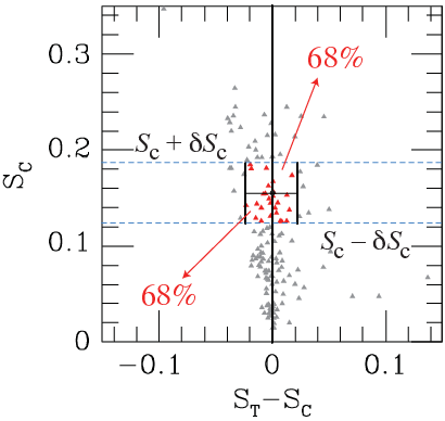
In Figure 6 we present the calibration for some (four) clusters of the sample, which were chosen because they represent different levels of substructure (from Abell 907 with $S_{C}=0.062$ to Abell 2163 with $S_{C}=0.155$ ) and different core radii and signal-to-noise. This figure shows both the measured against the true amount of substructure (left panel) and the corrected substructure level (central panel) and the method we used for computing the uncertainties on the substructure quantification (right panel). In Figure 7 we ilustrate the Monte Carlo simulation with a very small sub-sample of the images created to calibrate the method for Abell 85. On the top left we see its X-ray image, as observed by the Chandra Space Telescope, and its simulated images containing randomly distributed substructures.

{comment}

V.4.1 Examples of substructure identification: A586 and A2163

As an example and test of our method, we present here the case of two clusters, A586 and A2163, shown in Figs. 8 and 13. These X-ray images are in the $0.3$ – $7.0$ keV energy band.

In figure 8 we have the X-ray image in the left, the positive substructures in the center, defined as being the surface brightness excess with respect to the model fitted. In the same way, we define the negative substructure as lack of intensity with respect to the best fitted model; the negative substructures are shown in the right panel. The method applied to this cluster illustrates the detection of weak structures, that are very difficult to be identified by visual inspection, but may be of great importance in understanding some physical processes [20, see, e.g.,]. In figure 13 we have the same images as in figure 8, but for A2163.

Computing a temperature map based on Chandra data, Markevitch & Vikhlinin [23] clearly show that A2163 cluster is undergoing a major merging, while Cypriano et al. [6] suggest that A586 is probably a very relaxed cluster whose last major merger occurred more than $\approx 4$ Gyr ago. This is in agreement with the result of our analysis. Indeed, A586 presents the smallest substructure level of the sample, while A2163 presents a much higher substructure level, the highest of our sample.

In a work concerning the dark sector of the Universe, Bertolami et al. [1] show that the Abell 586 cluster exhibits evidence of the interaction between dark matter and dark energy based on the assumption of its relaxed state. The used the Layzer-Irvine equation which must hold for a system in virial equilibrium with no interaction between dark matter and energy, to show that if Abell 586 is indeed in equilibrium, this equation does not hold, thus indicating the existence of interaction in the dark sector. Abell 586 was chosen based on the work of Cypriano et al. [6] which suggests that A586 is probably a very relaxed cluster whose last major merger occurred more than $\approx 4$ Gyr ago. Our method could help these works by selecting clusters whose substructure level is low for further analysis.

VI Results and Discussion

Now that we have measured and corrected the substructure level and estimated the error bars within 68% confidencel level using Monte Carlo simulations, we may look for correlations between the substructure level, as we defined, and physical properties of the clusters.

For correlations to be correctly assessed, it is necessary to well understand how variables are related. Linear regression is a fundamental and frequently used tool in astronomy and it may seem surprising that such a statistical procedure, apparently simple, may be complicated and controversial [see, e.g., 13, 8, 11, for reviews]. Briefly, when the scientific question clearly asks how one variable depends on the other, it is more appropriate to use OLS $(Y|X)$ , Ordinary Least Square - the least square fit of the function Y(X), to quantify how the variables are correlated, with Y being the dependent variable. However, when the scientific question does not clearly identifies the dependent variable, then it is recommended the used of OLS (Bisector) which is the bisector between the OLS $(Y|X)$ and OLS $(X|Y)$ fits, the last case representing the fit inversion with respect to the variables.

With respect to the size of the sample, when the size is small ( $N<50$ , $N$ the number of data points), resampling methods such as Jackknife or Bootstrap should be used [8] to fit the data and estimate the uncertainties.

The correlation strength is estimated by the Pearson coefficient [31, see,], where its absolute value resides between 0 and 1, with 1 meaning total correlation and 0 none. The interpretation of the correlation strength depends on the context. A correlation of 0.9 may be very low if we are verifying a physical law with high quality equipments, but may be seen as very high in social sciences for example, where there are many contributions of complicated variables. In Table 1 we give the two-tailed null hypothesis significance for each Pearson correlation coefficient (See Press et al. [28] for more information on how it is computed).

In our case, we used the OLS $(Y|X)$ to fit relations between the substructure level and physical parameters, whereas we used the OLS (Bisector) for the scaling relations, all fits performed using the Jackknife resampling method.

Relation	Best Fit	Fit	Pearson	Null Hypothesis
$M_{500}$ - $T$	$M_{500}=0.312^{+0.039}_{-0.036}\times T^{1.64\pm 0.07}$	OLS (Bisector)	0.94	$<10^{-6}$
$L_{X}$ - $M_{500}$	$L_{X}=0.281^{+0.069}_{-0.055}\times M_{500}^{~~1.94\pm 0.17}$	OLS (Bisector)	0.89	$<10^{-6}$
$L_{X}$ - $T$	$L_{X}=0.029^{+0.013}_{-0.009}\times T^{3.20\pm 0.29}$	OLS (Bisector)	0.91	$<10^{-6}$
Scale Relations (High Substructure Level)
$M_{500}$ - $T$	$M_{500}=0.378^{+0.079}_{-0.065}\times T^{1.49\pm 0.10}$	OLS (Bisector)	0.92	$<10^{-6}$
$L_{X}$ - $M_{500}$	$L_{X}=0.424^{+0.145}_{-0.108}\times M_{500}^{~~2.03\pm 0.15}$	OLS (Bisector)	0.88	$<10^{-6}$
$L_{X}$ - $T$	$L_{X}=0.058^{+0.024}_{-0.017}\times T^{3.02\pm 0.18}$	OLS (Bisector)	0.90	$<10^{-6}$
Scale Relations (Low Substructure Level)
$S$ - $(1+z)$	$S=0.036^{+0.010}_{-0.007}\times(1+z)^{5.45\pm 1.95}$	OLS $\rm Y(X)$	0.35	0.042439
$S$ - $M_{500}$	$S=0.021^{+0.010}_{-0.007}\times M_{500}^{~~0.62\pm 0.20}$	OLS $\rm Y(X)$	0.49	0.003265
$S$ - $T$	$S=0.016^{+0.012}_{-0.007}\times T^{0.74\pm 0.30}$	OLS $\rm Y(X)$	0.36	0.036499
$S$ - $L_{X}$	$S=0.040^{+0.014}_{-0.010}\times L_{X}^{~~0.17\pm 0.10}$	OLS $\rm Y(X)$	0.26	0.137540
Substructure Level vs. Physical Parameters

Table 1: Table with best fits. Temperature is given in keV, mass in

10^{14}\rm M_{\odot}

and luminosity in

10^{44}\rm erg/s

VI.1 Clusters Parameters

In table 2 we give the corrected substructure level ( $S_{C}$ ), $M_{500}$ , X-ray luminosity, temperature, redshift, the 2D analytical surface brightness model fitted, core radius ( $R_{C}$ ) and signal-to-noise of the 34 clusters of the sample.

We computed the substructure level and the 2D analytical surface brightness model, while the other parameters were obtained from the literature [29, 32, 5, 24]. $M_{500}$ and X-ray luminosity were corrected to a Hubble constant of 70 km s^-1 Mpc^-1, and then X-ray luminosity was extrapolated to the bolometric band (0.01 - 100 keV) using K-correction and the XSPEC 12.0 MEKAL model (Mewe-Kaastra-Leidahl plasma emission code), since literature values were given for different Hubble constants and energy bands. Redshifts were obtained from NED (NASA/IPAC Extragalactic Database) with uncertanties varying from $10^{-6}$ to $10^{-4}$ , therefore as they are extremly small compared to other uncertainties we use, they are not displayed in Table 2.

Cluster	$S_{C}$	$M_{500},10^{14}\rm M_{\odot}$	$L_{X},10^{44}\rm erg~s^{-1}$	$kT$ , keV	$z$	Model	R	$R_{C}$	$S/N$
A85	$0.095^{+0.009}_{-0.007}$	5.77 $\pm$ 1.12	11.88 $\pm$ 0.30	$6.51^{+0.16}_{-0.23}$	0.055	$\beta$	C	9	735
A399	$0.101^{+0.055}_{-0.031}$	5.53 $\pm$ 1.54	8.72 $\pm$ 1.07	$6.46^{+0.38}_{-0.36}$	0.071	$\beta$	C	76	403
A401	$0.023^{+0.007}_{-0.008}$	5.99 $\pm$ 0.87	16.14 $\pm$ 0.65	$7.19^{+0.28}_{-0.24}$	0.074	$\beta$	C	55	360
A478	$0.065^{+0.016}_{-0.006}$	6.32 $\pm$ 2.14	22.16 $\pm$ 0.97	$6.91^{+0.40}_{-0.36}$	0.088	$\beta$	C	14	246
A520	$0.120^{+0.225}_{-0.038}$	7.83 $\pm$ 0.32	18.40 $\pm$ 0.25	$6.59^{+0.22}_{-0.23}$	0.199	$\beta$	M	77	195
A644	$0.077^{+0.038}_{-0.013}$	6.01 $\pm$ 1.54	10.28 $\pm$ 0.43	$6.54^{+0.27}_{-0.26}$	0.070	$\beta$	C	43	418
A665	$0.159^{+0.022}_{-0.018}$	9.62 $\pm$ 0.45	23.40 $\pm$ 0.26	$7.48^{+0.28}_{-0.28}$	0.182	Sérsic	M	17	175
A907	$0.062^{+0.010}_{-0.005}$	4.90 $\pm$ 0.23	11.50 $\pm$ 0.10	$5.16^{+0.10}_{-0.10}$	0.153	$\beta$	M	12	218
A1204	$0.043^{+0.013}_{-0.016}$	2.97 $\pm$ 0.23	9.95 $\pm$ 0.19	$3.41^{+0.07}_{-0.12}$	0.171	$\beta$	M	5	130
A1413	$0.052^{+0.005}_{-0.007}$	7.11 $\pm$ 0.28	17.10 $\pm$ 0.10	$7.21^{+0.16}_{-0.16}$	0.143	$\beta$	M	20	364
A1644	$0.152^{+0.027}_{-0.022}$	5.24 $\pm$ 3.07	4.04 $\pm$ 0.77	$4.70^{+0.90}_{-0.70}$	0.047	$\beta$	C	10	234
A1650	$0.034^{+0.008}_{-0.014}$	4.66 $\pm$ 1.55	8.35 $\pm$ 1.16	$5.68^{+0.30}_{-0.27}$	0.084	$\beta$	C	23	356
A1689	$0.051^{+0.006}_{-0.006}$	9.36 $\pm$ 0.59	39.40 $\pm$ 0.30	$9.02^{+0.27}_{-0.27}$	0.183	$\beta$	M	12	392
A1795	$0.099^{+0.008}_{-0.010}$	7.05 $\pm$ 2.75	11.92 $\pm$ 0.36	$6.17^{+0.26}_{-0.25}$	0.062	$\beta$	C	16	445
A1914	$0.112^{+0.040}_{-0.012}$	9.17 $\pm$ 0.63	34.30 $\pm$ 0.34	$9.59^{+0.33}_{-0.33}$	0.171	$\beta$	M	30	197
A2029	$0.021^{+0.006}_{-0.012}$	7.11 $\pm$ 2.35	23.50 $\pm$ 0.93	$7.93^{+0.39}_{-0.36}$	0.078	Sérsic	C	12	298
A2034	$0.092^{+0.117}_{-0.033}$	5.87 $\pm$ 0.19	9.41 $\pm$ 0.07	$6.59^{+0.15}_{-0.15}$	0.113	$\beta$	M	73	292
A2142	$0.023^{+0.059}_{-0.011}$	10.24 $\pm$ 2.60	30.13 $\pm$ 1.55	$8.46^{+0.53}_{-0.49}$	0.091	Sérsic	C	12	554
A2163	$0.155^{+0.022}_{-0.024}$	24.32 $\pm$ 1.82	93.90 $\pm$ 1.33	$14.70^{+0.87}_{-0.85}$	0.203	$\beta$	M	36	475
A2319	$0.085^{+0.090}_{-0.035}$	9.69 $\pm$ 1.54	24.05 $\pm$ 0.86	$8.84^{+0.29}_{-0.24}$	0.056	$\beta$	C	78	436
A2657	$0.040^{+0.010}_{-0.011}$	4.33 $\pm$ 0.94	1.56 $\pm$ 0.05	$3.53^{+0.12}_{-0.12}$	0.040	$\beta$	C	28	243
A3158	$0.038^{+0.032}_{-0.012}$	4.11 $\pm$ 0.64	6.23 $\pm$ 0.33	$5.41^{+0.26}_{-0.24}$	0.060	$\beta$	C	59	417
A3266	$0.137^{+0.036}_{-0.034}$	13.74 $\pm$ 3.40	11.68 $\pm$ 0.46	$7.72^{+0.35}_{-0.28}$	0.059	$\beta$	C	58	479
A3562	$0.055^{+0.019}_{-0.015}$	2.51 $\pm$ 0.31	3.09 $\pm$ 0.13	$4.47^{+0.23}_{-0.21}$	0.049	$\beta$	C	30	247
A3921	$0.077^{+0.015}_{-0.019}$	4.71 $\pm$ 1.07	5.35 $\pm$ 0.36	$5.39^{+0.38}_{-0.35}$	0.093	$\beta$	C	35	233
A4038	$0.004^{+0.026}_{-0.006}$	1.54 $\pm$ 0.06	1.67 $\pm$ 0.22	$3.15^{+0.03}_{-0.03}$	0.030	$\beta$	RB	37	456
ESO3060170-B $\dagger$	$0.082^{+0.014}_{-0.018}$	1.50 $\pm$ 0.50	0.65 $\pm$ 0.04	$2.63^{+0.05}_{-0.05}$	0.039	Sérsic	S	13	120
EXO0422	$0.033^{+0.006}_{-0.005}$	1.94 $\pm$ 1.22	1.68 $\pm$ 0.40	$2.90^{+0.90}_{-0.60}$	0.040	$\beta$	C	9	189
MKW 3S	$0.040^{+0.010}_{-0.005}$	2.30 $\pm$ 0.66	2.48 $\pm$ 0.09	$3.45^{+0.13}_{-0.10}$	0.045	$\beta$	C	23	528
MS 0906.5+1110	$0.112^{+0.015}_{-0.012}$	4.53 $\pm$ 0.25	9.01 $\pm$ 0.15	$5.19^{+0.17}_{-0.17}$	0.180	Sérsic	M	3	110
PKS0745-191	$0.032^{+0.005}_{-0.003}$	6.34 $\pm$ 0.25	35.90 $\pm$ 0.68	$7.21^{+0.11}_{-0.11}$	0.103	$\beta$	RB	11	251
RXCJ 1504-0248	$0.074^{+0.045}_{-0.026}$	9.81 $\pm$ 1.13	66.60 $\pm$ 0.72	$7.13^{+0.24}_{-0.24}$	0.109	Sérsic	M	1	187
RXJ1720.1+2638	$0.061^{+0.008}_{-0.009}$	6.83 $\pm$ 0.38	22.30 $\pm$ 0.23	$5.87^{+0.12}_{-0.12}$	0.164	$\beta$	M	7	199
ZWCL1215	$0.125^{+0.049}_{-0.051}$	6.76 $\pm$ 4.10	6.27 $\pm$ 1.73	$6.36^{+2.94}_{-2.01}$	0.075	$\beta$	C	66	193

Table 2: Clusters parameters. Core radius (

R_{C}

) is given in pixel units (whole image is 500

\times

500 pixels). Literature references (R) are given by: RB - Reiprich & Böhringer [29], S - Sun et al. [32], C - Chen et al. [5], M - Maughan et al. [24].

\dagger

The mass is given within

1/3R_{vir}

R_{vir}=1.35

Mpc.

VI.2 Substructure Level vs. Physical Parameters

Keeping in mind the different statistical approaches, for all the correlations between the substructure level and physical parameters the OLS $(Y|X)$ was used, since the substructure level may depend on mass, temperature and luminosity but these quantities should not be dependent on substructure, the way it was defined. For the scaling relations we used the OLS (Bisector) since temperature, luminosity and mass have complicated relations connecting them. For instance, mass is one of the quantities which determines the cluster temperature, but temperature is used to compute the mass. Luminosity is the observed quantity (flux and redshift), although it depends on temperature. Therefore complicated relations exist between them, which made us use the OLS (Bisector). On the other hand, concerning the data size, since we have used 34 data points we chose the Jackknife resampling method to perform all the fits. The results of the fits are presented in Table 1.

VI.2.1 Substructure Level vs. Redshift

Figure 11 shows the substructure level as a function of cluster redshift. We see that there is a dependence between the substructure level and redshift ( $S\propto(1+z)^{5.45\pm 1.95}$ ), although within $2.8\sigma$ we find no evolution at all in the substructure level. The dependence on redshift may be explained by the fact that nearby clusters fill a larger detector area compared to more distance clusters, and as explained in the calibration Section (§ V), they tend to have the substructure level understimated, since substructures that lie within small clustercentric distances are incorporated into the surface brightness fit and are hardly quantified. Furthermore the Pearson correlation coefficient of 0.35 shows us a weak correlation, which translates as no significant structural evolution of the gas distribution. We also note the strong scatter of the data points in the redshift range $z\in[0.02,0.2]$ , showing that we find clusters in very different dynamical states in this redshift interval, from those highly symmetrical to the very disturbed ones (see Figures 12 and 13). Such a scatter may be related to the young (dynamically speaking) age of massive clusters. Abell 4038, which has the smallest substructure level, has been considered in all fits, however we present in Figures 11, 14, 15 and 16 dashed lines representing the fits excluding it, since one could ask how much influence it has in determining the slopes of the curves.

Computing a temperature map based on Chandra data, Markevitch & Vikhlinin [23] clearly showed that Abell 2163 cluster (see Figure 13) is undergoing a major merger, which explains its high substructure level ( $SL=0.155^{+0.022}_{-0.024}$ ).

VI.2.2 Substructure Level vs. Temperature

We see in Figure 14 that hotter clusters show the tendency to present more substructures, however the Pearson coefficient of 0.36 shows a weak correlation. The slope of $0.74\pm 0.30$ shows a positive corrrelation within $2.5\sigma$ , however the weak correlation does not allow us to state any firm conclusion concerning the intensity of substrutures and gas temperature enhancements.

VI.2.3 Substructure Level vs. Luminosity

We see in Figure 15 that substructure is basically independent of X-ray luminosity, the Pearson coefficient of 0.26 being the lowest between the substructure level and the physical parameters. Furthermore, the substructure level is compatible with no dependency at all with the X-ray luminosity within only $1.7\sigma$ .

VI.2.4 Substructure Level vs. Mass

Figure 16 shows the substructure level as a function of the cluster mass. We see that more massive clusters show the tendency to present more substructures. The relation between the substructure level and the mass has the form $S\propto M^{0.62\pm 0.20}$ , with a positive correlation within $3.1\sigma$ , however, different from the temperature, luminosity and redshift correlations with the substructure level, the Pearson correlation coeficient is the largest (0.49) between them, presenting a strong (Null Hypothesis Significance= 0.003265 – there is only $\sim 0.3\%$ probability of not presenting correlation) relation between the amount of substructures a cluster presents and its mass.

{comment}

VI.2.5 Substructure Level vs. Metallicity

Figure 17 shows the substructure level as a function of the cluster gas metallicity. We see that there is no evidence of correlation between the level of substructure in the ICM gas and its metal abundance.

This lack of correlation implies that supernovae gas heating is not the main source of substructures, since the substructure level dependence with temperature is strong and, therefore, an increase in temperature due to supernova energy injection should be translated into a higher substructure level, which would be correlated with an increase in metellicity.

It is worth stressing that only 23 clusters were used [from 2008Maughan, who give the metallicity within $R_{500}$ ], and therefore the statistics is rather poor (not only in number of points, but also because of the data uncertainties) for us to rule out a possible correlation (or lack of) between metallicity and substructure level.

VI.3 Scaling Relations

Chen et al. [5] constructed two cluster samples based on the intra-cluster plasma central temperature, and they concluded that cooling-core clusters have different scaling relations compared to non-cooling-core clusters. Using the same idea, we created two different groups based on the substructure level. We computed the mean and median substructure level of the sample (illustrated in Figure 18). We choose the median, which is more robust regarding extreme data points, as a division line between high and low substructure level. Therefore, clusters were separated into two sub-groups according to their substructure level compared to the median value of the whole sample. Numerically, a cluster was considered highly substructured if its substructure level were greater than $S=0.069755$ , and a low substructure level cluster otherwise.

{comment}

$M_{500}$ - $T$ $M_{500}=0.312^{+0.039}_{-0.036}\times T^{1.64\pm 0.07}$ OLS (Bisector) 0.94
$L_{X}$ - $M_{500}$ $L_{X}=0.281^{+0.069}_{-0.055}\times M_{500}^{~~1.94\pm 0.17}$ OLS (Bisector) 0.89
$L_{X}$ - $T$ $L_{X}=0.029^{+0.013}_{-0.009}\times T^{3.20\pm 0.29}$ OLS (Bisector) 0.91
Scale Relations (High Substructure Level)
$M_{500}$ - $T$ $M_{500}=0.378^{+0.079}_{-0.065}\times T^{1.49\pm 0.10}$ OLS (Bisector) 0.92
$L_{X}$ - $M_{500}$ $L_{X}=0.424^{+0.145}_{-0.108}\times M_{500}^{~~2.03\pm 0.15}$ OLS (Bisector) 0.88
$L_{X}$ - $T$ $L_{X}=0.058^{+0.024}_{-0.017}\times T^{3.02\pm 0.18}$ OLS (Bisector) 0.90
Scale Relations (Low Substructure Level)

The cluster segregation in high and low substructure level shows that hotter clusters are distributed equaly between high and low substructure level clusters as well as the more massive and luminous clusters do not reside in a preferential group (high and low substructure groups).

The Pearson correlation strength coefficients for the scaling relations of these different groups are very similar, with the correlations for the high substructure group being slighly higher (roughly 0.01 above). The slopes are very similar also, with the excepction of the the $M-T$ relation being $1.23\sigma$ compatible, while the $L-T$ and $L-M$ relations are $0.53\sigma$ and $0.40\sigma$ compatibles, respectively. However, differently from Figure 19 in which the slope is similar and the intercept off-set between the curves is small, Figures 20 and 21 show a clear off-set ( $2.07\sigma$ and $2.23\sigma$ for $L-M$ and $L-T$ respectively) between the curves for high and low-substructure level clusters. It appears that given a fixed cluster temperature or mass, the luminosity expected for low-substructure clusters tend to be higher. A possible explanation may be that low-substructure clusters, therefore more relaxed ones, have had enough time for the gas to accomodate into the gravitational potential and become denser, which enhances the X-ray luminosity. Figure 6 of Chen et al. [5] shows a very similar effect, where their cool-core clusters present higher X-ray luminosities, for a fixed temperature, compared to non-cool-core clusters, which would advocate in favor of low-substructure clusters, and therefore more relaxed ones being associated with cool-core clusters.

The different scale relations between low-high substructure level clusters suggests that substructures are an important factor to bias scaling relations, therefore it may affect the mass of clusters determination and thus the mass function that is used to test cosmological models, e.g. using the Press-Schechter Extended model etc.

VII Conclusions

We have developed a new method to quantify X-ray substructures in clusters of galaxies based on the ratio between the number of counts in the residual and original X-ray images. We calibrated the method and then applied it to 34 clusters of galaxies in order to obtain the substructure level dependence with physical parameters, such as mass, temperature, X-ray luminosity and redshift.

The calibration was done using Monte Carlo simulations, which showed that the method recuperates very well the true amount of substructure for small angular core radii clusters (with respect to the whole image size) and good signal-to-noise ratio observations.

The substructure level high scatter (spanning from less than 1 to $\simeq 16\%$ ) in the redshift range $z\in[0.02,0.2]$ shows that clusters are found in all dynamical states in the local Universe: from those relaxed to completely disturbed.

We have not found any strong evidence of correlation between the substructure level and physical properties of the clusters, gas temperature, X-ray luminosity and redshift. However, there seems to be a correlation between the substructure level and the cluster mass, which is given by its Pearson correlation coeficient of 0.49. For our sample of 34 clusters it represents a probability of not presenting correlation of the order of $0.3\%$ .

The distinction between high and low substructure level clusters has shown to be interesting, since different scaling relations were found with these two sub-samples (they present an off-set of $\sim 2\sigma$ – given a fixed mass or temperature, low substructure clusters tend to be more X-ray luminous), which is an important result for cosmological tests which use the cluster mass-luminosity relation to compute the mass function.

A practical application of our method would be the identification of clusters of very low substructure level. Such relaxed clusters would be ideal laboratories for studies where the equilibrium hypothesis is of paramount importance. As an example, the work of Bertolami et al. (2007), on the interaction between dark matter and dark energy, made use of the Layzer-Irvine equation, which must hold for a system in virial equilibrium when there is no interaction in the dark sector. They applied their method to Abell 586, based on the analysis of Cypriano et al. (2005), which suggests that Abell 586 is indeed a very relaxed cluster.

Finally, it is important to say that the method itself is interesting since it concerns a new way to quantify substructures in clusters of galaxies, with a very simple physical interpretation: it reflects the fraction of the X-ray luminosity provided by substructures.

We are grateful to Ben Maughan, for kindly providing us with new results and Kristian Pedersen, Steen Hansen, Ralph Kraft, William Forman, Christine Jones, Eric Hallman, Cláudia Mendes, Hugo Capelato and Ronaldo E. de Souza for interesting discussions. We are also very grateful to the anonymous referee who helped a lot to improve this work. This work was supported by FAPESP (grants 2008/05970-0 and 2008/04318-7) and CNPq (Edital Universal 472012/2007-0). Facilities: Instituto de Astronomia, Geofísica e Ciências Atmosféricas - Universidade de São Paulo.

References

[1] Bertolami, O., Gil Pedro, F., & Le Delliou, M. 2007, Physics Letters B, 654, 165
[2] Buote, D. A., & Tsai, J. C. 1995, ApJ, 452, 522
[3] —. 1996, ApJ, 458, 27
[4] Cavaliere, A., & Fusco-Femiano, R. 1976, A&A, 49, 137
[5] Chen, Y., Reiprich, T. H., Böhringer, H., Ikebe, Y., & Zhang, Y.-Y. 2007, A&A, 466, 805
[6] Cypriano, E. S., Lima Neto, G. B., Sodré, Jr., L., Kneib, J.-P., & Campusano, L. E. 2005, ApJ, 630, 38
[7] Demarco, R., Magnard, F., Durret, F., & Márquez, I. 2003, A&A, 407, 437
[8] Feigelson, E. D., & Babu, G. J. 1992, ApJ, 397, 55
[9] Ferrari, C., Benoist, C., Maurogordato, S., Cappi, A., & Slezak, E. 2005, A&A, 430, 19
[10] Henriksen, M., Donnelly, R. H., & Davis, D. S. 2000, ApJ, 529, 692
[11] Hogg, D. W., Bovy, J., & Lang, D. 2010, arXiv:1008.4686
[12] Huchra, J. P., & Geller, M. J. 1982, ApJ, 257, 423
[13] Isobe, T., Feigelson, E. D., Akritas, M. G., & Babu, G. J. 1990, ApJ, 364, 104
[14] Jeltema, T. E., Canizares, C. R., Bautz, M. W., & Buote, D. A. 2005, ApJ, 624, 606
[15] Jeltema, T. E., Hallman, E. J., Burns, J. O., & Motl, P. M. 2008, ApJ, 681, 167
[16] Jones, C., & Forman, W. 1984, ApJ, 276, 38
[17] Jones, C., & Forman, W. 1992, in NATO ASIC Proc. 366: Clusters and Superclusters of Galaxies, ed. A. C. Fabian, 49–+
[18] —. 1999, ApJ, 511, 65
[19] Kauffmann, G., & White, S. D. M. 1993, MNRAS, 261, 921
[20] Laganá, T. F., Lima Neto, G. B., Andrade-Santos, F., & Cypriano, E. S. 2008, A&A, 485, 633
[21] Laganá, T. F., Andrade-Santos, F., & Lima Neto, G. B. 2010, A&A, 511, A15
[22] Lima Neto, G. B., Capelato, H. V., Sodré, Jr., L., & Proust, D. 2003, A&A, 398, 31
[23] Markevitch, M., & Vikhlinin, A. 2001, ApJ, 563, 95
[24] Maughan, B. J., Giles, P. A., Randall, S. W., Jones, C., & Forman, W. R. 2011, arXiv:1108.1200
[25] Mohr, J. J., Evrard, A. E., Fabricant, D. G., & Geller, M. J. 1995, ApJ, 447, 8
[26] Muanwong, O., Kay, S. T., & Thomas, P. A. 2006, ApJ, 649, 640
[27] Pislar, V., Durret, F., Gerbal, D., Lima Neto, G. B., & Slezak, E. 1997, A&A, 322, 53
[28] Press, W. H., Teukolsky, S. A., Vetterling, W. T., & Flannery, B. P. 1992, Cambridge: University Press, —c1992, 2nd ed.,
[29] Reiprich, T. H., & Böhringer, H. 2002, ApJ, 567, 716
[30] Richstone, D., Loeb, A., & Turner, E. L. 1992, ApJ, 393, 477
[31] Rodgers, J. L., & Nicewander, W. A. 1988, The American Statistician, 42, 59
[32] Sun, M., Forman, W., Vikhlinin, A., Hornstrup, A., Jones, C., & Murray, S. S. 2004, ApJ, 612, 805
[33] Suwa, T., Habe, A., Yoshikawa, K., & Okamoto, T. 2003, ApJ, 588, 7
[34] Xue, Y.-J., & Wu, X.-P. 2000, ApJ, 538, 65

{comment}

.1 Substructure Level Normalization

Taking into account the way the function $f(C_{i}^{r},A_{i})$ was defined, the numerator of the first term of equation (1) is written as:

\displaystyle F(C_{1}^{r},\ldots,C_{n}^{r},A_{1},\ldots,A_{n})\equiv\displaystyle\sum^{n}_{i=1}f(C_{i}^{r},A_{i})=\sum^{n}_{i=1}C_{i}^{r}\left(1+\frac{A_{i}}{A_{t}}\right).

(8)

The total area $A_{t}$ (from the image, given in pixels) is equal to $n$ , and defining the following sums as,

\displaystyle\chi\equiv\displaystyle\sum^{n}_{i=1}C_{i}^{r}~~~\rm and~~~\xi\equiv\displaystyle\sum^{n}_{i=1}A_{i},

(9)

equation (8) is written as:

\displaystyle F(C_{1}^{r},\ldots,C_{n}^{r},A_{1},\ldots,A_{n})\equiv\displaystyle\chi+\frac{1}{n}\sum^{n}_{i=1}C_{i}^{r}A_{i}.

(10)

Defining $F_{2}$ the second term of the right side of equation (10), we see that:

\displaystyle F_{2}(C_{1}^{r},\ldots,C_{n}^{r},A_{1},\ldots,A_{n})\equiv\displaystyle\frac{1}{n}\left[C_{1}^{r}A_{1}+\sum^{n}_{i=2}C_{i}^{r}A_{i}\right].

(11)

Injecting equations (9) into equation (11) we have:

\displaystyle F_{2}(C_{1}^{r},\ldots,C_{n}^{r},A_{1},\ldots,A_{n})\equiv\displaystyle\frac{1}{n}\left[\chi\xi+\sum^{n}_{i,j=2}C_{i}^{r}A_{j}-\xi\sum^{n}_{i=2}C_{i}^{r}-\chi\sum^{n}_{i=2}A_{i}+\sum^{n}_{i=2}C_{i}^{r}A_{i}\right].

(12)

Partially differentiating $F_{2}$ with respect to $C_{k}^{r}$ , $k\in[2,n]$ , we get:

\displaystyle\frac{\partial F_{2}(C_{1}^{r},\ldots,C_{n}^{r},A_{1},\ldots,A_{n})}{\partial C^{r}_{k}}=\displaystyle\frac{1}{n}\left[\sum^{n}_{i=2}A_{i}-\xi+A_{k}\right].

(13)

Taking the partial differential equals to 0, we get from the maximum (seeing that the minimum is 0) of function $F_{2}$ with respect to $C_{k}^{r}$ :

\displaystyle A_{k}=\xi-\sum^{n}_{i=2}A_{i}~,~\forall k\in[2,n].

(14)

However the second term is equal to $A_{1}$ , thus:

\displaystyle A_{k}=A_{1}~,~\forall k\in[2,n],

(15)

and therefore:

\displaystyle A_{i}=\frac{\xi}{n}~,~\forall i\in[1,n].

(16)

Doing the same for $C^{r}_{i}$ , we get:

\displaystyle C_{i}^{r}=\frac{\chi}{n}~,~\forall i\in[1,n],

(17)

and taking these values for $C_{i}^{r}$ and $A_{i}$ , $\forall i\in[1,n]$ , we have:

\displaystyle F(C_{1}^{r},\ldots,C_{n}^{r},A_{1},\ldots,A_{n})=\chi+\frac{\chi\xi}{n^{2}},

(18)

and for $F$ to be maximum, we should have $\xi=n^{2}$ , which is the maximum value for $\xi$ , thus:

\displaystyle 0\leq F(C_{1}^{r},\ldots,C_{n}^{r},A_{1},\ldots,A_{n})\leq 2\chi,

(19)

and considering that the denominator of the first term of equation (1) is always greater than $\chi$ , the first term of the same equation admits values between 0 and 2, therefore a factor of 1/2 normalizes it.

{comment}

Appendix A Clusters Parameters

In the following table we give the redshift, mass, X-ray luminosity, metallicity, temperature, substructure level and the 2D analytical surface brightness model fitted for the 34 clusters of the sample.

We computed the substructure level and the 2D analytical surface brightness model, while the other parameters were obtained from the literature [18, 29, 32, 5, 2008Maughan].

{comment}

Table 3: Clusters parameters.

Cluster	$S$	$M_{500}(10^{14}\rm M_{\odot})$	$L_{X}(10^{44}\rm erg/s)$	$T(\rm keV)$	$Z(\rm Z_{\odot})$	$z$	$Model$
A85	$0.0949^{+0.0092}_{-0.0074}$	11.31 $\pm$ 4.91	18.95 $\pm$ 0.22	6.51 $\pm$ 0.23	- $\pm$ -	0.055	$\beta$
A399	$0.101^{+0.055}_{-0.031}$	10.84 $\pm$ 3.25	13.97 $\pm$ 1.22	6.46 $\pm$ 0.38	- $\pm$ -	0.071	$\beta$
A401	$0.0226^{+0.0069}_{-0.0083}$	11.73 $\pm$ 3.97	24.32 $\pm$ 0.43	7.19 $\pm$ 0.28	- $\pm$ -	0.074	$\beta$
A478	$0.0653^{+0.016}_{-0.0062}$	12.39 $\pm$ 6.56	34.18 $\pm$ 0.35	6.91 $\pm$ 0.40	- $\pm$ -	0.088	$\beta$
A520	$0.120^{+0.23}_{-0.038}$	15.56 $\pm$ 3.11	17.60 $\pm$ 0.20	7.1 $\pm$ 0.2	0.42 $\pm$ 0.04	0.199	$\beta$
A644	$0.077^{+0.038}_{-0.013}$	11.77 $\pm$ 5.33	16.37 $\pm$ 0.29	6.54 $\pm$ 0.27	- $\pm$ -	0.070	$\beta$
A665	$0.159^{+0.022}_{-0.018}$	17.18 $\pm$ 3.44	21.00 $\pm$ 0.20	7.5 $\pm$ 0.2	0.34 $\pm$ 0.04	0.182	Sérsic
A907	$0.0616^{+0.010}_{-0.0052}$	8.89 $\pm$ 1.78	10.40 $\pm$ 0.10	5.3 $\pm$ 0.1	0.49 $\pm$ 0.03	0.153	$\beta$
A1204	$0.043^{+0.013}_{-0.016}$	5.11 $\pm$ 1.02	9.20 $\pm$ 0.20	3.4 $\pm$ 0.1	0.37 $\pm$ 0.05	0.171	$\beta$
A1413	$0.0523^{+0.0053}_{-0.0069}$	12.44 $\pm$ 2.49	15.90 $\pm$ 0.10	7.2 $\pm$ 0.2	0.41 $\pm$ 0.03	0.143	$\beta$
A1644	$0.152^{+0.022}_{-0.027}$	10.27 $\pm$ 6.16	7.68 $\pm$ 0.67	4.7 $\pm$ 0.9	- $\pm$ -	0.047	$\beta$
A1650	$0.0336^{+0.0083}_{-0.014}$	9.14 $\pm$ 3.40	14.37 $\pm$ 1.55	5.68 $\pm$ 0.30	- $\pm$ -	0.084	$\beta$
A1689	$0.0509^{+0.0061}_{-0.0058}$	17.18 $\pm$ 3.44	36.70 $\pm$ 0.30	9.0 $\pm$ 0.3	0.42 $\pm$ 0.04	0.183	$\beta$
A1795	$0.0994^{+0.0078}_{-0.010}$	13.81 $\pm$ 7.67	19.60 $\pm$ 0.14	6.17 $\pm$ 0.26	- $\pm$ -	0.062	$\beta$
A1914	$0.112^{+0.040}_{-0.012}$	16.87 $\pm$ 3.37	32.60 $\pm$ 0.30	9.8 $\pm$ 0.3	0.34 $\pm$ 0.05	0.171	$\beta$
A2029	$0.0214^{+0.0061}_{-0.012}$	13.93 $\pm$ 7.22	33.46 $\pm$ 0.36	7.93 $\pm$ 0.39	- $\pm$ -	0.078	Sérsic
A2034	$0.092^{+0.12}_{-0.033}$	10.70 $\pm$ 2.14	9.00 $\pm$ 0.10	6.7 $\pm$ 0.2	0.38 $\pm$ 0.04	0.113	$\beta$
A2107	$0.0458^{+0.0042}_{-0.0067}$	2.65 $\pm$ 0.50	1.49 $\pm$ 0.05	4.1 $\pm$ 0.2	- $\pm$ -	0.041	$\beta$
A2142	$0.023^{+0.059}_{-0.011}$	20.06 $\pm$ 9.56	41.26 $\pm$ 0.57	8.46 $\pm$ 0.53	- $\pm$ -	0.091	Sérsic
A2163	$0.155^{+0.022}_{-0.024}$	44.55 $\pm$ 8.91	87.80 $\pm$ 1.30	15.5 $\pm$ 0.9	0.43 $\pm$ 0.09	0.203	$\beta$
A2319	$0.085^{+0.090}_{-0.035}$	18.99 $\pm$ 6.42	32.08 $\pm$ 0.51	8.84 $\pm$ 0.29	- $\pm$ -	0.056	$\beta$
A2657	$0.040^{+0.010}_{-0.011}$	8.48 $\pm$ 3.59	3.41 $\pm$ 0.06	3.53 $\pm$ 0.12	- $\pm$ -	0.040	$\beta$
A2670	$0.108^{+0.019}_{-0.024}$	2.40 $\pm$ 0.50	2.01 $\pm$ 0.10	3.9 $\pm$ 0.2	- $\pm$ -	0.076	$\beta$
A3158	$0.038^{+0.032}_{-0.012}$	8.05 $\pm$ 2.32	11.00 $\pm$ 0.29	5.41 $\pm$ 0.26	- $\pm$ -	0.060	$\beta$
A3266	$0.137^{+0.036}_{-0.034}$	26.93 $\pm$ 10.61	16.90 $\pm$ 0.22	7.72 $\pm$ 0.35	- $\pm$ -	0.059	$\beta$
A3562	$0.055^{+0.019}_{-0.015}$	4.91 $\pm$ 1.27	6.04 $\pm$ 0.10	4.47 $\pm$ 0.23	- $\pm$ -	0.049	$\beta$
A3921	$0.077^{+0.014}_{-0.019}$	9.22 $\pm$ 3.24	9.47 $\pm$ 0.27	5.39 $\pm$ 0.38	- $\pm$ -	0.093	$\beta$
A4038	$0.0037^{+0.026}_{-0.0062}$	3.02 $\pm$ 0.12	0.50 $\pm$ 0.01	3.22 $\pm$ 0.10	- $\pm$ -	0.030	$\beta$
ESO3060170-B	$0.082^{+0.014}_{-0.018}$	1.50 $\pm$ 0.50	0.25 $\pm$ 0.12	2.63 $\pm$ 0.05	- $\pm$ -	0.039	Sérsic
EXO0422	$0.0330^{+0.0056}_{-0.0055}$	3.80 $\pm$ 2.39	3.98 $\pm$ 0.41	2.90 $\pm$ 0.90	- $\pm$ -	0.040	$\beta$
MKW 3S	$0.0398^{+0.0099}_{-0.0046}$	4.50 $\pm$ 2.14	5.47 $\pm$ 0.10	3.45 $\pm$ 0.13	- $\pm$ -	0.045	$\beta$
MS 0906.5+1110	$0.112^{+0.015}_{-0.012}$	7.95 $\pm$ 1.59	8.40 $\pm$ 0.10	5.3 $\pm$ 0.2	0.31 $\pm$ 0.07	0.180	Sérsic
PKS0745-191	$0.0318^{+0.0055}_{-0.0035}$	7.27 $\pm$ 0.75	28.20 $\pm$ 0.60	7.97 $\pm$ 0.28	- $\pm$ -	0.103	$\beta$
RXCJ 1504-0248	$0.074^{+0.045}_{-0.026}$	14.18 $\pm$ 2.83	61.10 $\pm$ 0.60	6.8 $\pm$ 0.2	0.35 $\pm$ 0.04	0.109	Sérsic
RXJ1720.1+2638	$0.0606^{+0.0083}_{-0.0086}$	12.29 $\pm$ 2.45	19.80 $\pm$ 0.20	6.1 $\pm$ 0.1	0.48 $\pm$ 0.03	0.164	$\beta$
ZWCL1215	$0.125^{+0.049}_{-0.051}$	9.46 $\pm$ 5.74	5.17 $\pm$ 0.11	6.36 $\pm$ 2.94	- $\pm$ -	0.075	$\beta$

{comment}

Table 4: Clusters parameters. Literature references are given by: JF - Jones & Forman [18], RB - Reiprich & Böhringer [29], S - Sun et al. [32], C - Chen et al. [5], M - 2008Maughan

Cluster	$S$	$M_{500}(10^{14}\rm M_{\odot})$	$L_{X}(10^{44}\rm erg/s)$	$T(\rm keV)$	$z$	Model	Reference
A85	$0.0949^{+0.0092}_{-0.0074}$	11.31 $\pm$ 4.91	18.95 $\pm$ 0.22	6.51 $\pm$ 0.23	0.055	$\beta$	C
A399	$0.101^{+0.055}_{-0.031}$	10.84 $\pm$ 3.25	13.97 $\pm$ 1.22	6.46 $\pm$ 0.38	0.071	$\beta$	C
A401	$0.0226^{+0.0069}_{-0.0083}$	11.73 $\pm$ 3.97	24.32 $\pm$ 0.43	7.19 $\pm$ 0.28	0.074	$\beta$	C
A478	$0.0653^{+0.016}_{-0.0062}$	12.39 $\pm$ 6.56	34.18 $\pm$ 0.35	6.91 $\pm$ 0.40	0.088	$\beta$	C
A520	$0.120^{+0.23}_{-0.038}$	15.56 $\pm$ 3.11	17.60 $\pm$ 0.20	7.1 $\pm$ 0.2	0.199	$\beta$	M
A644	$0.077^{+0.038}_{-0.013}$	11.77 $\pm$ 5.33	16.37 $\pm$ 0.29	6.54 $\pm$ 0.27	0.070	$\beta$	C
A665	$0.159^{+0.022}_{-0.018}$	17.18 $\pm$ 3.44	21.00 $\pm$ 0.20	7.5 $\pm$ 0.2	0.182	Sérsic	M
A907	$0.0616^{+0.010}_{-0.0052}$	8.89 $\pm$ 1.78	10.40 $\pm$ 0.10	5.3 $\pm$ 0.1	0.153	$\beta$	M
A1204	$0.043^{+0.013}_{-0.016}$	5.11 $\pm$ 1.02	9.20 $\pm$ 0.20	3.4 $\pm$ 0.1	0.171	$\beta$	M
A1413	$0.0523^{+0.0053}_{-0.0069}$	12.44 $\pm$ 2.49	15.90 $\pm$ 0.10	7.2 $\pm$ 0.2	0.143	$\beta$	M
A1644	$0.152^{+0.022}_{-0.027}$	10.27 $\pm$ 6.16	7.68 $\pm$ 0.67	4.7 $\pm$ 0.9	0.047	$\beta$	C
A1650	$0.0336^{+0.0083}_{-0.014}$	9.14 $\pm$ 3.40	14.37 $\pm$ 1.55	5.68 $\pm$ 0.30	0.084	$\beta$	C
A1689	$0.0509^{+0.0061}_{-0.0058}$	17.18 $\pm$ 3.44	36.70 $\pm$ 0.30	9.0 $\pm$ 0.3	0.183	$\beta$	M
A1795	$0.0994^{+0.0078}_{-0.010}$	13.81 $\pm$ 7.67	19.60 $\pm$ 0.14	6.17 $\pm$ 0.26	0.062	$\beta$	C
A1914	$0.112^{+0.040}_{-0.012}$	16.87 $\pm$ 3.37	32.60 $\pm$ 0.30	9.8 $\pm$ 0.3	0.171	$\beta$	M
A2029	$0.0214^{+0.0061}_{-0.012}$	13.93 $\pm$ 7.22	33.46 $\pm$ 0.36	7.93 $\pm$ 0.39	0.078	Sérsic	C
A2034	$0.092^{+0.12}_{-0.033}$	10.70 $\pm$ 2.14	9.00 $\pm$ 0.10	6.7 $\pm$ 0.2	0.113	$\beta$	M
A2107	$0.0458^{+0.0042}_{-0.0067}$	2.65 $\pm$ 0.50 $\dagger$	1.49 $\pm$ 0.05	4.1 $\pm$ 0.2	0.041	$\beta$	JF
A2142	$0.023^{+0.059}_{-0.011}$	20.06 $\pm$ 9.56	41.26 $\pm$ 0.57	8.46 $\pm$ 0.53	0.091	Sérsic	C
A2163	$0.155^{+0.022}_{-0.024}$	44.55 $\pm$ 8.91	87.80 $\pm$ 1.30	15.5 $\pm$ 0.9	0.203	$\beta$	M
A2319	$0.085^{+0.090}_{-0.035}$	18.99 $\pm$ 6.42	32.08 $\pm$ 0.51	8.84 $\pm$ 0.29	0.056	$\beta$	C
A2657	$0.040^{+0.010}_{-0.011}$	8.48 $\pm$ 3.59	3.41 $\pm$ 0.06	3.53 $\pm$ 0.12	0.040	$\beta$	C
A2670	$0.108^{+0.019}_{-0.024}$	2.40 $\pm$ 0.50 $\dagger$	2.01 $\pm$ 0.10	3.9 $\pm$ 0.2	0.076	$\beta$	JF
A3158	$0.038^{+0.032}_{-0.012}$	8.05 $\pm$ 2.32	11.00 $\pm$ 0.29	5.41 $\pm$ 0.26	0.060	$\beta$	C
A3266	$0.137^{+0.036}_{-0.034}$	26.93 $\pm$ 10.61	16.90 $\pm$ 0.22	7.72 $\pm$ 0.35	0.059	$\beta$	C
A3562	$0.055^{+0.019}_{-0.015}$	4.91 $\pm$ 1.27	6.04 $\pm$ 0.10	4.47 $\pm$ 0.23	0.049	$\beta$	C
A3921	$0.077^{+0.014}_{-0.019}$	9.22 $\pm$ 3.24	9.47 $\pm$ 0.27	5.39 $\pm$ 0.38	0.093	$\beta$	C
A4038	$0.0037^{+0.026}_{-0.0062}$	3.02 $\pm$ 0.12	0.50 $\pm$ 0.01	3.22 $\pm$ 0.10	0.030	$\beta$	RB
ESO3060170-B	$0.082^{+0.014}_{-0.018}$	1.50 $\pm$ 0.50 $\dagger$	0.25 $\pm$ 0.12	2.63 $\pm$ 0.05	0.039	Sérsic	S
EXO0422	$0.0330^{+0.0056}_{-0.0055}$	3.80 $\pm$ 2.39	3.98 $\pm$ 0.41	2.90 $\pm$ 0.90	0.040	$\beta$	C
MKW 3S	$0.0398^{+0.0099}_{-0.0046}$	4.50 $\pm$ 2.14	5.47 $\pm$ 0.10	3.45 $\pm$ 0.13	0.045	$\beta$	C
MS 0906.5+1110	$0.112^{+0.015}_{-0.012}$	7.95 $\pm$ 1.59	8.40 $\pm$ 0.10	5.3 $\pm$ 0.2	0.180	Sérsic	M
PKS0745-191	$0.0318^{+0.0055}_{-0.0035}$	7.27 $\pm$ 0.75	28.20 $\pm$ 0.60	7.97 $\pm$ 0.28	0.103	$\beta$	RB
RXCJ 1504-0248	$0.074^{+0.045}_{-0.026}$	14.18 $\pm$ 2.83	61.10 $\pm$ 0.60	6.8 $\pm$ 0.2	0.109	Sérsic	M
RXJ1720.1+2638	$0.0606^{+0.0083}_{-0.0086}$	12.29 $\pm$ 2.45	19.80 $\pm$ 0.20	6.1 $\pm$ 0.1	0.164	$\beta$	M
ZWCL1215	$0.125^{+0.049}_{-0.051}$	9.46 $\pm$ 5.74	5.17 $\pm$ 0.11	6.36 $\pm$ 2.94	0.075	$\beta$	C

A New Method to Quantify X-ray Substructures in Clusters of Galaxies

Abstract

Keywords:

I Introduction

II Sample Definition

III Data Reduction and Analysis

III.1 Data Reduction

III.2 Surface Brightness

IV X-ray Substructures

IV.1 Substructure Level

V Calibration of the Method

V.1 General Case

V.2 Long Exposure Time Observation

V.3 Short Exposure Time Observation

V.4 Monte Carlo Simulations

V.4.1 Examples of substructure identification: A586 and A2163

VI Results and Discussion

VI.1 Clusters Parameters

VI.2 Substructure Level vs. Physical Parameters

VI.2.1 Substructure Level vs. Redshift

VI.2.2 Substructure Level vs. Temperature

VI.2.3 Substructure Level vs. Luminosity

VI.2.4 Substructure Level vs. Mass

VI.2.5 Substructure Level vs. Metallicity

VI.3 Scaling Relations

VII Conclusions

References

.1 Substructure Level Normalization

Appendix A Clusters Parameters

A New Method to Quantify X-ray Substructures in
Clusters of Galaxies