IPPP-11-83
DCPT-11-166
models of tri-bimaximal-reactor mixing
Abstract
Recent results from T2K, MINOS and Double CHOOZ all indicate a sizeable reactor angle which would rule out conventional tri-bimaximal lepton mixing. However, it is possible to maintain the tri-bimaximal solar and atmospheric mixing angle predictions, , even for a quite sizeable reactor angle , using an ansatz called tri-bimaximal-reactor (TBR) mixing proposed by one of us some time ago. We propose an explicit model of leptons based on the type I seesaw mechanism at both the effective and the renormalisable level which, together with vacuum alignment, leads to surprisingly accurate TBR neutrino mixing, with the second order corrections to mixing angles having small coefficients.
1 Introduction
Recently T2K have published evidence for a large non-zero reactor angle [1] which, when combined with data from MINOS and other experiments in a global fit yields [2],
| (1.1) |
where the reactor angle is defined in the usual PDG convention [3] and the errors indicate the one range, although the statistical significance of a non-zero reactor angle is about 3. A non-zero reactor angle is also consistent with the first results from Double CHOOZ [4].
If confirmed, these recent observations would rule out conventional tri-bimaximal (TB) mixing which predicts a zero reactor angle [5]. Many alternative proposals [6] have been put forward since the first T2K results, all aiming to accommodate a non-zero . Typically, such models also yield (sizable) deviations to the other predictions of TB mixing, namely tri-maximal solar mixing and maximal atmospheric mixing . However, since the latter remain in good agreement with current global fits [2], it would be nice if, somehow, these good predictions of TB mixing could be maintained while at the same time allowing a non-zero reactor angle. In fact the idea of maintaining the TB predictions for the solar and atmospheric angles, while switching on the reactor angle, was suggested some time ago (before T2K results) by one of us and was referred to as tri-bimaximal-reactor (TBR) mixing [7].
The TBR ansatz [7] postulates a free reactor angle but with fixed and corresponding to tri-maximal solar mixing and maximal atmospheric mixing . In the PDG convention for the PMNS mixing matrix [3] the TBR ansatz for the mixing matrix is then [7],
where contains the usual Majorana phases. Note that TBR mixing reduces to TB mixing in the limit that . However in general TBR mixing involves an arbitrary reactor angle which could in principle be large, without causing any deviations from TB solar and atmospheric mixing and .
The TBR ansatz in Eq. (1) is clearly very simple to write down. The obvious question is whether there is any model that can give rise to TBR mixing. Such a model of TBR mixing should also explain the smallness of the reactor angle as compared to the tri-maximal solar mixing angle and the maximal atmospheric mixing angle . At the same time that the TBR ansatz was proposed, a mechanism was suggested called partially constrained sequential dominance (PCSD) which could lead to TBR mixing [7]. Although no actual model was proposed, it was shown how PCSD could originate due to a distortion of the vacuum alignment which was previously used to account for TB mixing via constrained sequential dominance (CSD), which in turn could originate from family symmetry [7].
In this paper we propose the first explicit model of leptons based on the type I seesaw mechanism at both the effective and the renormalisable level which, together with vacuum alignment, leads to PCSD and hence TBR mixing. To understand the approach we are following in this paper, it is useful to first recall the CSD approach to TB mixing. The basic ingredients there are sequential dominance (SD) [8, 9] and vacuum alignment. The strategy of combining SD with vacuum alignment is familiar from the CSD approach to TB mixing [10] where a neutrino mass hierarchy is assumed and the dominant and subdominant flavons responsible for the atmospheric and solar neutrino masses are aligned in the directions of the second and third columns of the TB mixing matrix, namely and . The idea of PCSD [7] is to simply maintain the subdominant flavon alignment, , while considering a small perturbation to the dominant flavon alignment, . Assuming PCSD, with a strong neutrino mass hierarchy, , leads to a perturbed neutrino mass matrix [7],
| (1.6) |
where and are the leading order neutrino mass eigenvalues. The explicit models we propose involve the accurate flavon alignments and which appear quadratically and reproduce the neutrino mass matrix as in Eq. (1.6) quite accurately in the case of the renormalisable model.
Another important result of our paper concerns the analytic diagonalisation of the neutrino mass matrix in Eq. (1.6) to second order . Previously it has been shown that, to leading order in and , Eq.(1.6) leads to TBR mixing in Eq. (1) [7, 11]. Remarkably, we find that the coefficients of the second order corrections to the mixing angles are suppressed, making the approximate TBR mixing resulting from Eq. (1.6) to be more accurate than expected. Thus the renormalisable model predicts surprisingly accurate TBR mixing with , even for quite sizeable .
We note that PCSD is based on the general approach to model building known as the indirect approach [12] which involves the quadratic appearance of the flavons as in Eq. (1.6). Recently an alternative type of model of TBR mixing has been proposed based on family symmetry, with a type I plus type II seesaw mechanism, although no detailed model was proposed and the necessary vacuum alignment was not studied [13]. Moreover, TBR mixing does not follow in a general way from the model in [13], but only occurs for special choices of parameters.
The layout of the rest of the paper is as follows. In Section 2 we propose an explicit model of leptons at both the effective and the renormalisable level which, together with vacuum alignment, leads to PCSD and hence TBR mixing. In Section 3 we give the results of the analytic diagonalisation of the neutrino mass matrix in Eq. (1.6) to second order . The straightforward generalisation to the case with a non-zero lightest neutrino mass is presented in Appendix A and might be relevant for some future model. Section 4 concludes the paper.
2 models of tri-bimaximal-reactor mixing
In this section we present the details of the model, first at the effective, then at the renormalisable level. As pointed out in the introduction, our models follow the indirect approach and the aligned flavons appear quadratically in the light neutrino mass matrix as in Eq.(1.6). In order to achieve this via the type I see-saw mechanism, and to ensure a diagonal charged lepton mass matrix, additional shaping symmetries are also employed. In such models, the discrete family symmetry is pivotal in two aspects: it () helps generate the required flavon alignments and () combines the three generations into multiplets of the group so that, together with the corresponding product rules, one obtains mass matrices which depend on only a few free parameters. In this paper we choose to work with as it is the smallest non-Abelian finite group with an irreducible triplet representation. We apply the basis in which the triplets are explicitly real as given for example in [14]. Denoting a general triplet as and defining , the product rules can be summarised as
| (2.1) |
corresponding to two triplets and the sum of the three one-dimensional irreducible representations , with being the trivial singlet. Furthermore, .
2.1 The effective model
The complete list of lepton, Higgs and flavon fields introduced in our model is given in Table 1. Similar to the model of [15] we have a symmetry as well as several shaping symmetries.
The neutrino part of the effective superpotential reads,
| (2.2) |
where the effectively allowed mixing term must be forbidden by the choice of appropriate messengers. Notice that there are only two right-handed neutrinos living in the singlet representation of . Hence, the model will feature one massless light neutrino. Inserting the flavon VEVs
| (2.3) |
whose alignment is discussed later, leads to the following Dirac and right-handed Majorana neutrino mass matrices
| (2.4) |
where and . Note that is diagonal by construction.
Using the type I seesaw formula we can express the light neutrino mass matrix as
| (2.5) |
With this structure we arrive at TBR mixing in the neutrino sector as will be shown analytically in Section 3.
In order to account for the charged lepton mass hierarchy we identify the right-handed charged leptons with singlets, and distinguish them using the shaping symmetries. The resulting effective charged lepton superpotential then takes the form
| (2.6) |
Inserting the flavon VEVs
| (2.7) |
whose alignment is discussed later leads to
| (2.8) |
thus yielding a diagonal charged lepton mass matrix . In this model, the hierarchy in the charged leptons remains unaccounted for, however it is straightforward to implement the Froggatt-Nielsen mechanism [16] to cure this. For the purpose of clarity we will ignore this issue in the following.
2.2 The renormalisable model
As emphasised in [17], any non-renormalisable operator of an effective superpotential should be understood in terms of a more fundamental underlying renormalisable theory. Without such a UV completion of a model, higher order terms which are allowed by the symmetries may or may not be present. Thus a purely effective formulation would leave room for different physical predictions. We have constructed a fully renormalisable theory of the lepton sector. The required messengers are listed in Table 2, while the driving fields which control the alignment of the flavons are presented in Table 3.
With the particle content and the symmetries specified in Tables 1-2, we can replace the effective neutrino superpotential in Eq. (2.2) by a renormalisable one which includes the messenger fields,
| (2.9) | |||||
Integrating out the messenger pairs and , the effective operators of Eq. (2.2) are uniquely generated. Notice that the messenger pairs , do not lead to the aforementioned mixing term .
The charged lepton sector is formulated at the renormalisable level using only one new pair of messengers, and . With the particles and symmetries listed in Tables 1 and 2 we get the renormalisable superpotential for the charged leptons
| (2.10) |
where we have suppressed all order one coupling constants. Integrating out the messengers, we are led uniquely to of Eq. (2.6).
2.3 Vacuum alignment
So far we have only postulated the particular alignments of the neutrino-type flavons, given in Eq. (2.3), and the flavons of the charged lepton sector, Eq. (2.7). In this subsection we explore the driving potential and prove that the assumed flavon alignments can in fact be obtained in a relatively simple and elegant way.
The renormalisable superpotential involving the driving fields necessary for aligning the neutrino-type flavons is given as
| (2.11) | |||||
The first line of Eq. (2.11) produces the vacuum alignment of Eq. (2.3) as can be seen from the -term conditions11 1 We remark that the general alignment derived from these -term conditions is . One can, however, show that all of them are equivalent as the resulting mass matrices will be related by appropriate changes of the unphysical phases in the matrix . Our choice leads to all being zero in the limit of vanishing , see Eqs. (3.13-3.15).
| (2.12) |
The terms in the second line of Eq. (2.11) give rise to orthogonality conditions which uniquely fix the alignments of the auxiliary flavon fields and ,
| (2.13) | |||||
| (2.14) |
Here we have assumed the flavons and to be already aligned as in Eqs. (2.7) and (2.3), respectively. Finally, the neutrino-type flavon gets aligned by the remaining terms of Eq. (2.11). A vanishing -term of the driving field requires
| (2.15) |
where and are independent parameters. They are further constrained by the -term condition of the driving field which – after integrating out the messenger pair and inserting the flavon VEVs – reads,
| (2.16) |
This shows that is naturally suppressed compared to due to the messenger mass. With , we get
| (2.17) |
as anticipated in Eq. (2.3).
Turning to the flavon alignment of the charged lepton sector, the renormalisable driving superpotential takes the form
| (2.18) |
Here we have suppressed all order one coefficients as they are completely irrelevant.
The triplet driving fields give rise to flavon alignments with two zero components. The singlet driving fields in turn require orthogonality among the three flavon VEVs so that we end up with the vacuum structure of Eq. (2.7), possibly requiring some redefinition of the family indices.
3 Analytic diagonalisation of the PCSD neutrino mass matrix to second order
In this section we diagonalise the effective neutrino mass matrix of Eq. (1.6),
| (3.1) |
which arises in the indirect models of Section 2, see Eq. (2.5). Numerically the complex parameter
| (3.2) |
, is assumed to take an absolute value of . It is therefore reasonable to expand the mixing matrix which diagonalises in powers of . In the limit of vanishing , the absolute values of the mass parameters
| (3.3) |
correspond to the eigenvalues of , and the mixing matrix is exactly of tri-bimaximal form. Switching on changes both the masses and the mixing. In what follows we assume a normal hierarchical neutrino mass spectrum which allows us to parameterise the masses in Eq. (3.1) as
| (3.4) |
with being an order one coefficient. The neutrino mass matrix of Eq. (3.1) is now diagonalised by the unitary mixing matrix such that22 2 Here we assume the convention in which the effective light neutrino mass matrix is defined through the bilinear coupling, in contrast to the convention adopted in [7].
| (3.5) |
is an unphysical phase matrix which is required to bring the PMNS matrix into PDG form,
| (3.6) |
with and . The Majorana phases are included in the matrix .
We have worked out the mixing matrix to second order in using the above notation. The results read
| (3.7) | |||||
| (3.8) | |||||
| (3.9) | |||||
| (3.10) | |||||
| (3.11) | |||||
| (3.12) | |||||
| (3.13) | |||||
| (3.14) | |||||
| (3.15) |
leading to a diagonalised mass matrix of the form
| (3.16) |
Notice that the Dirac CP phase is only given to first order in as it always appears together with whose leading term is already suppressed by one power of . The Majorana phases on the other hand do not receive any corrections of order or . With there is only one physical Majorana phase,
| (3.17) |
To first order in the deviations in the solar and atmospheric mixing vanish, and only the reactor angle is switched on. Hence the mass matrix of Eq. (3.1) gives rise to TBR mixing at leading order. In more detail, the second order results show that the solar mixing angle is corrected to values slightly smaller than the TB value, while the atmospheric angle can deviate to larger or smaller values, depending on the phases. Furthermore, the deviation of is bigger by a factor of about compared to the deviation of .
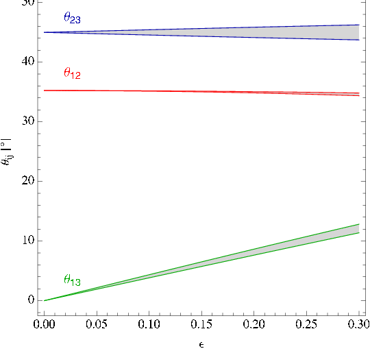
Our analytic expressions confirm the numerical results for PCSD obtained with the Mixing Parameter Tools of the REAP Mathematica package [18]. The resulting variation of the mixing angles with is shown in Fig. 1. The broadening of the allowed regions of the atmospheric and reactor mixing angles is caused by the phase dependence of and , cf. Eqs. (3.8,3.9). In the case of the solar mixing angle, our analytic formula, Eq. (3.7), does not show any phase dependence to second order in , so the significantly smaller broadening of the allowed region of is an effect of third order in .
We can express our results in terms of the deviation parameters , and as defined in [19],
| (3.18) |
Comparing these definitions with our second order expressions in Eqs. (3.7-3.12) we find
| (3.19) |
where we have replaced the original phase parameters by the two physical phases and , keeping only terms up to second order in . These relations can be combined to yield the second order sum rules
| (3.20) |
Using these sum rules and the second order expansion of the PMNS matrix given in [19], we can rewrite the mixing matrix of PCSD in terms of the reactor deviation parameter and the parameter ,
| (3.21) |
The comparison with the second order expansion of the TBR mixing matrix in Eq. (1), where ,
illustrates how accurately TBR mixing is achieved in models of PCSD.
It is also worth noting that the columns of the Dirac mass matrix in Eq.(2.4) are not quite proportional to the columns of the PMNS matrix in Eq.(3.21), so that form dominance [20] is violated at order . This implies that leptogenesis is non-zero [21], even in the absence of renormalisation group corrections [22].
4 Conclusions
Recent results from T2K, MINOS and Double CHOOZ all indicate a sizeable reactor angle which would rule out conventional tri-bimaximal lepton mixing. However, it is possible to maintain the tri-bimaximal solar and atmospheric mixing angle predictions, , even for a quite sizeable reactor angle such as , using an ansatz called tri-bimaximal-reactor (TBR) mixing in Eq. (1) proposed by one of us some time ago, along with the neutrino mass matrix in Eq. (1.6) arising from PCSD [7].
In this paper we have proposed the first explicit model of leptons based on the type I seesaw mechanism at both the effective and the renormalisable level which, together with vacuum alignment, leads to the desired form of neutrino mass matrix. After performing an analytic diagonalisation of the neutrino mass matrix to second order, we find that the coefficients of the second order terms are suppressed, making TBR mixing surprisingly accurate for the renormalisable model. The analytic results are confirmed by the numerical results in Fig. 1 which illustrates the stability of the atmospheric and solar angles as the reactor angle is switched on.
It is worth emphasising that the models are indirect models involving the quadratic appearance of misaligned flavons as in Eq. (1.6). Moreover there is no simple Klein symmetry that is respected by this mass matrix; in fact, formally, the generators of the Klein symmetry involve the real order one parameter of Eq. (3.4), thus proving the absence of a direct link between the family symmetry and the Klein symmetry of the neutrino mass matrix. Nevertheless, the alignments of the flavons can readily originate from a simple discrete symmetry such as , which is broken in a rather complicated way in the neutrino sector, although the charged lepton sector is diagonal in the model of leptons considered here.
In a more complete family unified model, for example based on , one would expect the charged lepton sector to be related to the off-diagonal quark mass matrices, resulting in additional charged lepton corrections to the lepton mixing angles, together with renormalisation group (RG) corrections, as discussed in [23]. However it is worth emphasising that, typically, such corrections to mixing angles are not expected to exceed about 3∘ from charged lepton corrections and about 1∘ from RG corrections [23]. Such corrections are not sufficient to account for the observed reactor angle, although they may affect the predictions of TBR mixing discussed here, which strictly apply to the unrenormalised neutrino mixing angles only.
Acknowledgements
We are very grateful to Stefan Antusch for generously creating and donating the Figure, as well as for helpful correspondence. The authors acknowledge support from the STFC Rolling Grant No. ST/G000557/1 and partial support by the EU ITN grant UNILHC 237920 (Unification in the LHC era).
Appendix
Appendix A Analytic diagonalisation of the PCSD neutrino mass matrix with to second order
In this appendix we present the results of the mixing angles and phases for the more general case with three non-zero mass parameters . The starting point is the PCSD form of neutrino mass matrix with non-vanishing , namely,
| (A.1) |
Clearly, in the limit , this reduces to the PCSD form of neutrino mass matrix considered in Eq. (1.6) and Section 3. Adopting the notation of Section 3 and assuming the hierarchy
| (A.2) |
with being coefficients of order one or smaller, we obtain to second order in ,
| (A.3) | |||||
| (A.4) | |||||
| (A.5) | |||||
| (A.6) | |||||
| (A.7) | |||||
| (A.8) | |||||
| (A.9) | |||||
| (A.10) | |||||
| (A.11) |
The resulting neutrino masses read
| (A.12) |
Note that can be of same order in as without changing the mixing matrix to first order in . That is even with being of order one, we still find TBR mixing. Considering, however, the case where is additionally suppressed by one or more powers of , i.e. , the above expressions simplify considerably. Then, in fact, the dependence drops out completely to second order in , and we recover the expressions of Section 3, with corresponding to and set to zero.
References
- [1] K. Abe et al. [T2K Collaboration], Phys. Rev. Lett. 107 (2011) 041801 [arXiv:1106.2822].
- [2] G. L. Fogli, E. Lisi, A. Marrone, A. Palazzo and A. M. Rotunno, Phys. Rev. D 84 (2011) 053007 [arXiv:1106.6028]; T. Schwetz, M. Tortola and J. W. F. Valle, New J. Phys. 13 (2011) 109401 [arXiv:1108.1376].
- [3] K. Nakamura et al. [ Particle Data Group Collaboration ], J. Phys. G G37 (2010) 075021.
- [4] Talk by H. De Kerret at the LowNu conference in Seoul, Korea, Wednesday 9 November 2011.
- [5] P. F. Harrison, D. H. Perkins and W. G. Scott, Phys. Lett. B 530 (2002) 167 [hep-ph/0202074].
- [6] H. -J. He, F. -R. Yin, Phys. Rev. D84 (2011) 033009 [arXiv:1104.2654]; Z.-Z. Xing, arXiv:1106.3244; N. Qin and B. Q. Ma, Phys. Lett. B 702 (2011) 143 [arXiv:1106.3284]; Y. j. Zheng and B. Q. Ma, arXiv:1106.4040; E. Ma and D. Wegman, Phys. Rev. Lett. 107 (2011) 061803 [arXiv:1106.4269]; X. -G. He and A. Zee, Phys. Rev. D 84 (2011) 053004 [arXiv:1106.4359]; S. Zhou, Phys. Lett. B704 (2011) 291 [arXiv:1106.4808]; T. Araki, Phys. Rev. D84 (2011) 037301 [arXiv:1106.5211]; N. Haba, R. Takahashi, Phys. Lett. B702 (2011) 388 [arXiv:1106.5926]; D. Meloni, JHEP 1110 (2011) 010 [arXiv:1107.0221]; W. Chao, Y.-J. Zheng, arXiv:1107.0738; H. Zhang, S. Zhou, Phys. Lett. B704 (2011) 296 [arXiv:1107.1097]; X. Chu, M. Dhen and T. Hambye, JHEP 1111 (2011) 106 [arXiv:1107.1589]; P. S. Bhupal Dev, R. N. Mohapatra, M. Severson, Phys. Rev. D84 (2011) 053005 [arXiv:1107.2378]; R. d. A. Toorop, F. Feruglio, C. Hagedorn, Phys. Lett. B703 (2011) 447 [arXiv:1107.3486]; S. Antusch, V. Maurer, arXiv:1107.3728; S. F. King and C. Luhn, JHEP 1109 (2011) 042 [arXiv:1107.5332]; Q. -H. Cao, S. Khalil, E. Ma, H. Okada, Phys. Rev. D84 (2011) 071302 [arXiv:1108.0570]; D. Marzocca, S. T. Petcov, A. Romanino and M. Spinrath, JHEP 1111 (2011) 009 [arXiv:1108.0614]; S. F. Ge, D. A. Dicus and W. W. Repko, arXiv:1108.0964; F. Bazzocchi, arXiv:1108.2497; S. Antusch, S. F. King, C. Luhn and M. Spinrath, arXiv:1108.4278; P. O. Ludl, S. Morisi and E. Peinado, arXiv:1109.3393; A. Aranda, C. Bonilla and A. D. Rojas, arXiv:1110.1182; D. Meloni, arXiv:1110.5210; S. Dev, S. Gupta, R. R. Gautam and L. Singh, Phys. Lett. B 706 (2011) 168 [arXiv:1111.1300]; A. Rashed, arXiv:1111.3072; R. d. A. Toorop, F. Feruglio and C. Hagedorn, arXiv:1112.1340.
- [7] S. F. King, Phys. Lett. B 675 (2009) 347 [arXiv:0903.3199].
- [8] S. F. King, Phys. Lett. B 439 (1998) 350 [hep-ph/9806440]; S. F. King, Nucl. Phys. B 562 (1999) 57 [hep-ph/9904210]; S. F. King, Nucl. Phys. B 576 (2000) 85 [hep-ph/9912492]; S. F. King, JHEP 0209 (2002) 011 [hep-ph/0204360].
- [9] S. Antusch, S. Boudjemaa and S. F. King, JHEP 1009 (2010) 096 [arXiv:1003.5498].
- [10] S. F. King, JHEP 0508 (2005) 105 [hep-ph/0506297].
- [11] S. F. King, JHEP 1101 (2011) 115 [arXiv:1011.6167].
- [12] S. F. King and C. Luhn, JHEP 0910 (2009) 093 [arXiv:0908.1897].
- [13] S. Morisi, K. M. Patel and E. Peinado, Phys. Rev. D 84 (2011) 053002 [arXiv:1107.0696].
- [14] E. Ma and G. Rajasekaran, Phys. Rev. D 64 (2001) 113012 [hep-ph/0106291]; G. Altarelli and F. Feruglio, Nucl. Phys. B 720 (2005) 64 [hep-ph/0504165]; C. Luhn, S. Nasri and P. Ramond, J. Math. Phys. 48 (2007) 073501 [hep-th/0701188].
- [15] S. Antusch, S. F. King, C. Luhn and M. Spinrath, Nucl. Phys. B 850 (2011) 477 [arXiv:1103.5930].
- [16] C. D. Froggatt and H. B. Nielsen, Nucl. Phys. B 147 (1979) 277.
- [17] I. de Medeiros Varzielas and L. Merlo, JHEP 1102 (2011) 062 [arXiv:1011.6662].
- [18] S. Antusch, J. Kersten, M. Lindner, M. Ratz and M. A. Schmidt, JHEP 0503 (2005) 024 [hep-ph/0501272].
- [19] S. F. King, Phys. Lett. B 659 (2008) 244 [arXiv:0710.0530].
- [20] M. -C. Chen and S. F. King, JHEP 0906 (2009) 072 [arXiv:0903.0125].
- [21] S. Antusch, S. F. King and A. Riotto, JCAP 0611 (2006) 011 [hep-ph/0609038]; S. Choubey, S. F. King and M. Mitra, Phys. Rev. D 82 (2010) 033002 [arXiv:1004.3756].
- [22] I. K. Cooper, S. F. King and C. Luhn, arXiv:1110.5676.
- [23] S. Boudjemaa and S. F. King, Phys. Rev. D 79 (2009) 033001 [arXiv:0808.2782]; S. Antusch, S. F. King and M. Malinsky, Nucl. Phys. B 820 (2009) 32 [arXiv:0810.3863].