Generalized Hoeffding-Sobol Decomposition for Dependent Variables - Application to Sensitivity Analysis
Abstract
In this paper, we consider a regression model built on dependent variables. This regression modelizes an input output relationship. Under boundedness type assumptions on the joint distribution function of the input variables, we show that a generalized Hoeffding-Sobol decomposition is available. This leads to new indices measuring the sensitivity of the output with respect to the input variables. We also study and discuss the estimation of these new indices.
keywords
Sensitivity index , Hoeffding decomposition , dependent variables , Sobol decompositionUniversité de Grenoble, LJK/MOISE BP 53, 38041 Grenoble Cedex, France
??
Université Paul Sabatier, IMT-EPS, 118, Route de Narbonne, 31062 Toulouse Cedex 9, France
??
Université Joseph Fourier, LJK/MOISE BP 53, 38041 Grenoble Cedex, France
??
Contents
1 Introduction
Sensitivity analysis (SA) aims to identify the variables that most contribute to the variability into a non linear regression model.
Global SA is a stochatic approach whose objective is to determine a global criterion based on the density of the joint probability distribution function of the output
and the inputs of the regression model. The most usual quantification is the variance-based method, widely studied in SA literature.
Hoeffding decomposition [9] (see also Owen [21]) states that the variance of the output can be uniquely decomposed into summands of increasing dimensions under orthogonality constraints. Following this approach, Sobol [26] introduces variability measures, the so called Sobol sensitivity indices. These indices quantify the contribution of each input on the system.
Different methods have been exploited to estimate Sobol indices. The Monte Carlo algorithm was proposed by Sobol [27], and has been later improved by the Quasi Monte Carlo technique, performed by Owen [22]. FAST methods are also widely used to estimate Sobol indices. Introduced earlier by Cukier et al. [3] [4], they are well known to reduce the computational cost of multidimensional integrals thanks to Fourier transformations. Later, Tarantola et al. [29] adapted the Random Balance Designs (RBD) to FAST method for SA (see also recent advances on the subject by Tissot et al. [30]).
However, these indices are constructed on the hypothesis that input variables are independent, which seems unrealistic for many real life phenomena. In the literature, only a few methods and estimation procedures have been proposed to handle models with dependent inputs. Several authors have proposed sampling techniques to compute marginal contribution of inputs to the outcome variance (see the introduction in Mara and references therein [17]). As underlined in Mara et al.[17], if inputs are not independent, the amount of the response variance due to a given factor may be influenced by its dependence to other inputs. Therefore, classical Sobol indices and FAST approaches for dependent variables are difficult to interpret (see, for example, Da Veiga’s illustration [5] p.133). Xu and Gertner [32] proposed to decompose the partial variance of an input into a correlated part and an uncorrelated one. Such an approach allows to exhibit inputs that have an impact on the output only through their strong correlation with other incomes. However, they only investigated linear models with linear dependences.
Later, Li et al. [15] extended this approach to more general models, using the concept of High Dimensional Model Representation (HDMR [14]). HDMR is based on a hierarchy of component functions of increasing dimensions (truncation of Sobol decomposition in the case of independent variables). The component functions are then approximated by expansions in terms of some suitable basis functions (e.g., polynomials, splines, …). This meta-modeling approach allows the splitting of the response variance into a correlative contribution and a structural one of a set of inputs. Mara et al. [17] proposed to decorrelate the inputs with the Gram-Schmidt procedure, and then to perform the ANOVA-HDMR of Li et al. [15] on these new inputs. The obtained indices can be interpreted as fully, partially correlated and independent contributions of the inputs to the output. Nevertheless, this method does not provide a unique orthogonal set of inputs as it depends on the order of the inputs in the original set. Thus, a large number of sets has to be generated for the interpretation of resulting indices. As a different approach, Borgonovo et al. [1, 2] initiated the construction of a new generalized moment free sensitivity index. Based on geometrical consideration, these indices measure the shift area between the outcome density and this same density conditionally to a parameter. Thanks to the properties of these new indices, a methodology is given to obtain them analytically through test cases.
Notice that none of these works has given an exact and unambiguous definition of the functional ANOVA for correlated inputs as the one provided by Hoeffding-Sobol decomposition when inputs are independent. Consequently, the exact form of the model has neither been exploited to provide a general variance-based sensitivity measures in the dependent frame.
In a pionnering work, Hooker [10], inspired by Stone [28], shed new lights on hierarchically orthogonal function decomposition.
We revisit and extend here the work of Hooker. We obtain hierarchical functional decomposition under a general assumption on the inputs distribution.
Furthermore, we also show the uniqueness of the decomposition leading to the definition of new sensitivity indices.
Under suitable conditions on the joint distribution function of the input variables, we give a hierarchically orthogonal functional decomposition (HOFD) of the model.
The summands of this decomposition are functions depending only on a subset of input variables and are hierarchically uncorrelated. This means that two of these components are orthogonal whenever all the variables involved in one of the summands also appear in the other. This decomposition leads to the construction of generalized sensitivity indices well tailored to perform global SA when the input variables are dependent.
In the case of independent inputs, this decomposition is nothing more than the Hoeffding one. Furthermore, our generalized sensitivity indices are in this case the classical Sobol ones. In the general case, the computation of the summands of the HOFD involves a minimization problem under constraints (see Proposition 1).
A statistical procedure to approach the solution of this counstrainted optimization problem will be investigated in a next paper.
Here, we will focus on the particular case where the inputs are independent pairs of dependent variables (IPDV).
Firstly, in the simplest case of a single pair of dependent variables, the HOFD may be performed by solving a functional linear system
of equations involving suitable projection operators (see Procedure 4.1). In the
more general IPDV case, the HOFD is then obtained in two steps (see Procedure
4.2). The first step is a classical Hoeffding-Sobol decomposition of the output on
the input pairs, as developped in Jacques et al. [11]. The second step is the
HOFDs of all the pairs. In practical situations, the non parametric regression
function of the model is generally not exactly known. In this case, one can
only have at hand some realizations of the model and have to estimate, with
this information, the HOFD. Here, we study this statistical problem in the
IPDV case. We build estimators of the generalized sensitivity indices and study
numerically their properties. One of the main conclusion is that the
generalized indices have a total normalized sum. This is not true for classical
Sobol indices in the frame of dependent variables.
The paper is organized as follows.
In Section 2, we give and discuss general results on the HOFD. The main result
is Theorem 1. We show here that a HOFD is available under a boundedness type
assumption (2.3) on the density of the joint distribution function of the inputs. Further,
we introduce the generalized indices.
In Section 3, we give examples of multivariate distributions to which Theorem 1 applies. We also state a sufficient condition for (2.3) and necessary and sufficient conditions in the IDPV case.
Section 4 is devoted to the estimation procedures of the components of the HOFD and of the new sensitivity indices.
Section 5 presents numerical applications.
Through three toy functions, we estimate generalized indices and compare their
performances with the analytical values. In Section 6, we give conclusions and
discuss future work. Technical proofs and further details are postponed to the
Appendix.
2 Generalized Hoeffding decomposition-Application to SA
To begin with, let introduce some notation. We briefly recall the usual functional ANOVA decomposition, and Sobol indices. We then state a generalization of this decomposition, allowing to deal with correlated inputs.
2.1 Notation and first assumptions
We denote by the strict inclusion, that is , whereas we use when equality is possible.
Let be a probability space and let be the output of a deterministic model . Suppose that is a function of a random vector , and that is the pushforward measure of by ,
Let be a –finite measure on . Assume that and let be the density of with respect to , that is .
Also, assume that . The associated innner product of this Hilbert space is:
Here denotes the expectation. The corresponding norm will be classically denoted by .
Further, denotes the variance,
and the covariance.
Let and be the collection of all subsets of .
Define as the collection of all subsets of except itself.
Further, let , . We introduce the subspaces of , and . is the set of all measurable and square integrable functions depending only on . is the set of constants and is identical to . , , and are defined as follows:
At this stage, we do not make assumptions on the support of . For , the support of is denoted by .
2.2 Sobol sensitivity indices
In this section, we recall the classical Hoeffding-Sobol decomposition, and the Sobol sensitivity indices if the inputs are independent, that is when .
The usual presentation is done when [26], but the Hoeffding decomposition remains true in general case [31].
Let and assume that . The decomposition consists in writting as the sum of increasing dimension functions:
| (1) | |||||
The expansion (1) exists and is unique under one of the hypothesis:
Equation (1) tells us that the model function can be expanded in a functional ANOVA. The independence of the inputs and the orthogonality properties ensure the global variance decomposition of the output as .
Moreover, by integration, each term has an explicit expression, given by:
| (2) |
Hence, the contribution of a group of variables in the model can be quantified in the fluctuations of . The Sobol indices expressions are defined by:
| (3) |
Furthermore,
However, the main assumption is that the input parameters are independent. This is unrealistic in many cases.
The use of expressions previously set up is not excluded in case of inputs’ dependence,
but they could lead to an unobvious and sometimes a wrong interpretation.
Also, technics exploited to estimate them may mislead final results because most of them are built on the hypothesis of independence.
For these reasons, the objective of the upcoming work is to show that the construction of sensitivity indices under dependence condition can be done into a mathematical frame.
In the next section, we propose a generalization of the Hoeffding decomposition under suitable conditions on the joint distribution function of the inputs. This decomposition consists of summands of increasing dimension, like in Hoeffding one. But this time, the components are hierarchically orthogonal instead of being mutually orthogonal. The hierarchical orthogonality will be mathematically defined further. Thus, the global variance of the output could be decomposed as a sum of covariance terms depending on the summands of the HOFD. It leads to the construction of generalized sensitivity indices summed to to perform well tailored SA in case of dependence.
2.3 Generalized decomposition for dependent inputs
We no more assume that is a product measure. Nevertheless, we assume:
(C.1)
Our main assumption is :
(C.2)
where denotes the complement set of in . and are respectively the marginal densities of and .
The section is organized as follows: a preliminary lemma gives the main result to show that is a complete space.
Then, this ensures the existence and the uniqueness of the projection of onto .
The generalized decomposition of is finally obtained by adding a residual term orthogonal to every summand, as suggested in [10].
The first part of the reasoning is mostly inspired by Stone’s work [28], except that our assumptions are more general.
Indeed, we have a relaxed condition on the inputs distribution function.
Moreover, the support of is general.
To begin with, let us state some definitions. In the usual ANOVA context, a model is said to be hierarchical if for every term involving some inputs, all lower-order terms involving a subset of these inputs also appear in the model. Correspondingly, a hierarchical collection of subsets of is defined as follows:
Definition 1.
A collection is hierarchical if for and a subset of , one has .
The next Lemma is a generalization of the Lemma 3.1 of [28]. As already mentioned, it will be the key to show the hierarchical decomposition.
Lemma 1.
| (4) |
The proof of Lemma 1 is postponed to the Appendix. Our main theorem follows:
Theorem 1.
Let be any function in . Then, under (2.3) and (2.3), there exist functions such that the following equality holds :
| (5) | |||||
Moreover, this decomposition is unique.
The proof is given in the Appendix.
Notice that, in case where the input variables are independent, and Inequality (4) of Lemma 1 is an equality. Indeed, in this case, this equality is directly obtained by orthogonality of the summands.
The variational counterpart of Theorem 1 is a minimization problem under conditional constraints.
Proposition 1.
Then admits a unique solution .
Proof of Proposition 1 is postponed to the Appendix. Notice that a similar result for the Lebesgue measure is given in [10]. Its purpose was to provide diagnostics for high-dimensional functions. Here, we will no more exploit this idea. This will be done in a forthcoming work. Instead, we are going to construct stochastic sensitivity indices based on the new decomposition (5) and focus on a specific estimation method for IPDV models.
2.4 Generalized sensitivity indices
As stated in Theorem 1, under (2.3) and (2.3), the output of the model can be uniquely decomposed as a sum of hierarchically orthogonal terms. Thus, the global variance has a simplified decomposition into a sum of covariance terms. So, we can define generalized sensitivity indices.
Definition 2.
The sensitivity index of order measuring the contribution of into the model is given by :
| (6) |
More specifically, the first order sensitivity index is given by :
| (7) |
An immediate consequence is given in Proposition 2 (see proof in the Appendix) :
Proposition 2.
| (8) |
Thus, sensitivity indices are summed to . Furthermore, the covariance terms included in these new indices allow to take into account the inputs dependence. Thus, we are now able to measure the influence of a variable on the model, especially when a part of its variability is embedded
into the one of other dependent terms. We can distinguish the full contribution of a variable and its contribution into another correlated income.
Note that for independent inputs, the summands are mutually orthogonal, so , , and we recover the well known Sobol indices. Hence, these new sensitivity indices can be seen as a generalization of Sobol indices.
3 Examples of distribution function
This section is devoted to examples of distribution function satisfying (2.3) and (2.3). The first hypothesis only implies that the reference measure is a product of measures, whereas the second is trickier to obtain.
In the first part, we give a sufficient condition to get (2.3) for any number of input variables. The second part deals with the case , for which we give equivalences of (2.3) in terms of copulas.
3.1 Boundedness of the inputs density function
The difficulty of Condition (2.3) is that the inequality has to be true for any splitting of the set into two disjoint blocks. We give a sufficient condition for (2.3) to hold in Proposition 3 (the proof is postponed to the Appendix):
Let give now an example where (3) is satisfied.
Example 1: Let be the multidimensional gaussian distribution with
Assume that is a Gaussian mixture , with
Then, (3) holds iff the matrix is positive definite.
In the next section, we will see that (2.3) has a copula version when . We will give some examples of distribution satisfying one of these conditions.
3.2 Examples of distribution of two inputs
Here, we consider the simpler case of inputs . Also, until Section 4, we will assume that is absolutely continuous with respect to Lebesgue measure. The structure of dependence of and can be modelized by copulas. Copulas [19] give a relationship between a joint distribution and its marginals. Sklar’s theorem [25] ensures that for any distribution function with marginal distributions and , has the copula representation,
where the measurable function is unique whenever and are absolutely continuous.
The next corollary gives in the absolutely continuous case the relationship between a joint density and its marginal:
Corollary 1.
In terms of copulas, the joint density of is given by:
| (9) |
Furthermore,
| (10) |
Now, Condition (2.3) may be rephrased in terms of copulas:
Proposition 4.
For a two-dimensional model, the three following conditions are equivalent:
- 1.
(C.4)
- 2.
(C.5)
- 3.
for some copula (C.6)
The proof of Proposition 4 is postponed to the Appendix.
Hence, the generalized Hoeffding decomposition holds for a wide class of examples. The first example is the Morgenstern copulas [18]:
Let now consider the class of Archimedian copulas,
| (11) |
where the generator is a non negative two times differentiable function defined on with , and .
Proposition 5.
The proof is straightforward. Now, we will see three illustrative Archimedian copulas satisfying (2).
Example 3: The Frank copula is characterized by the generator:
Condition (2) holds, and if , elsewhere.
Example 4: Let , and with . Set
| (14) |
Example 5: Let and set
| (15) |
Leaving the class of copulas, we now directly work with the joint density function. Proposition 6 gives a general form of distribution for our framework:
Proposition 6.
If has the form
| (16) |
where , are univariate density functions, and is any density function (with respect to ) with marginals and , then satisfies (2).
The proof is straightforward.
Example 6: As an illustration of Proposition 6, take , a normal density with a diagonal covariance matrix , and a normal density of covariance matrix , with , .
Notice that because a copula of Gaussian mixture distribution is a mixture of Gaussian copulas (see [20]), this example can be directly recovered by the copula approach.
Example 7: Let generalize Example 3.2. If is a Gaussian mixture
with
then (1) holds iff and .
Thus, for many distributions, the generalized decomposition holds, and generalized sensitivity indices may thus be defined.
For the remaining part of the paper, we will assume that the set of inputs is an IPDV.
If is odd, we will assume that an input variable is independent to all the others.
The next section is devoted to the estimation of HOFD components. The simplest case of a single pair of dependent variables is first discussed.
Then, the more general IPDV case is studied.
In this last part, first and second order indices are defined to measure the contribution of each pair of dependent variables and each of its components in the model.
Indices of order greater than one involving variables from different pairs will not not be studied here.
4 Estimation
Using the property of hierarchical orthogonality (, ), we will see that the summands of the decomposition are solution of a functional linear system.
For , the projection operator onto is denoted by .
In this section, we present the HOFD terms computation, based on the resolution of a functional linear system. The result relies on projection operators previously set up. Further, we expose the linear system estimation for practice.
4.1 Models of input variables
This part is devoted to the simple case of bidimensional models. Let
Procedure 1
- 1.
HOFD of the output:
(17) - 2.
Projection of on , . As , , we obtain:
(18) - 3.
Computation of the right-hand side vector of (18):
(19) In this frame, we have:
- 4.
Reduction of the system (18). As the constant term corresponds to the expected value of , and the residual one can be deduced from the others, the dimension of the system (20) can even be reduced to:
(21) - 5.
Practical resolution: The numerical resolution of (21) is achieved by an iterative Gauss Seidel algorithm [13] which consists first in decomposing as a sum of lower triangular () and strictly upper triangular () matrices.
Further, the technique uses an iterative scheme to compute . At step , we have:
(22) Using expression of , we get:
(23) - 6.
Convergence of the algorithm: now, we hope that the Gauss Seidel algorithm converges to the true solution. Looking back at (18) , we see that we only have to consider (respectively ) restricted to (respectively to ).
Under this restriction, let us define the associated norm operator as :
As explained in [7], Gauss Seidel algorithm converges to the true solution if is striclty diagonally dominant, which is implied by :
(24) i.e.
(25) Equality (19) reveals that . Hence, by the Jensen inequality [12] for conditional expectations, admits an upper bound:
Take :
The same holds for , and we also have .
Moreover, the Jensen’s inequality is strict if is not -measurable. As is a function of (that is if and conversely), the condition of convergence holds if is not a measurable function of . Hence, Gauss Seidel algorithm converges if is not a function of . - 7.
Estimation procedure: Suppose that we get a sample of observations .
- •
Estimation of the components of the HOFD: the iterative scheme (23) requires to estimate conditional expectations. As extended in Da Veiga et al [6], we propose to estimate them by local polynomial regression at each point of observation. Then, we use the leave-one-out technique to set the learning sample and the test sample. Moreover, as the local polynomial method can be summed up to a generalized least squares (see Fan and Gijbels [8]), the Sherman-Morrison formula [24] is applied to reduce the computational time.
A more detailed procedure is given in the Appendix. The iterative algorithm is easy to implement. We stop when , for a small positive .Once have been estimated, we estimate by the empirical mean of the output. Then, an estimation of is obtained by substraction.
- •
We use empirical variance and covariance estimation to estimate sensitivity indices , and .
- •
4.2 Generalized IPDV models
Assume that the number of inputs is even, so , . We note each group of dependent variables as , . By rearrangement, we may assume that:
SA for IPDV models has already been treated in [11].
Indeed, they proposed to estimate usual sensitivity indices on groups of variables via Monte Carlo estimation.
Thus, they have interpreted the influence of every group of variables on the global variance.
Here, we will go further by trying to measure the influence of each variable on the output, but also the effets of the independent pairs.
To begin with, as a slight generalization of [26] and used in [11], let apply the Sobol decomposition on groups of dependent variables,
where for and , we set .
Furthermore, , .
Thus, we obtain independent components of IPDV. Under the assumptions discussed in the previous section, we can apply the HOFD of each of these components, that is,
with , . In this way, let define some new generalized indices for IPDV models:
Definition 3.
For , the first order sensitivity index measuring the contribution of (respectively ) on the output of the model is:
| (26) |
The second order sensitivity index for the pair , , is defined as:
| (27) |
The estimation procedure of these indices is quite similar to Procedure 4.1:
Procedure 2
- 1.
- 2.
If is odd, the procedure is the same except that the influence of the independent variable is measured by a Sobol index, as it is independent from all the others.
The next part is devoted to numerical examples.
5 Numerical examples
In this section, we study three examples with dependent input variables.
We consider IPDV models and a Gaussian mixture distribution on the input variables.
We choose covariance matrices of the mixture satisfying conditions of Example 3.1.
We give estimations of our new indices, and compare them to the analytical ones, computed from expressions (6). We also compute dispersions of the estimated new indices.
In [6], Da Veiga et al. proposed to estimate the classical Sobol indices , by nonparametric tools.
Indeed, the local polynomial regression were used to estimate conditional moments . This method, used further, will be called Da Veiga procedure (DVP).
Results given by DVP are compared with the ones given by our method.
The goal is to show that the usual sensitivity indices are not appropriate in the dependence frame, even if a relevant estimation method is used.
5.1 Two-dimensional IPDV model
Let consider the model
Here, and are of the form given by Example 3.1, with .
Thus, the analytical decomposition of is
For the application, we implement Procedure 4.1 in Matlab software.
We proceed to simulations and observations.
Parameters were fixed at , , and .
In Table 1, we give the estimation of our indices and their standard deviation (indicated by ) on simulations. In comparison, we give the analytical value of each index.
The analytical classical Sobol indices are difficult to obtain, but we give estimators of the classical Sobol indices with DVP.
| New indices | Estimation | ||||
| Analytical | |||||
| DVP indices | Estimation |
We notice that estimations with our method give quite good results in comparison with their analytical values. The estimation error of the interaction term is due to the fact that the component is obtained by difference between the output and the other estimated components.
The DVP indices are are difficult to interpret as the sum is higher than .
In our method, it would be relevant to separate the variance part to the covariance one in the first order indices. Indeed, in this way, we would be able to get the part of variability explained by alone in , and its contribution hidden in the dependence with . We note the variance contribution alone, and the covariance contribution, that is
The new indices estimations given in Table 1 are decomposed in Table 2. As previously, the number at the right of indicates the standard deviation on simulations.
| Analytical |
|---|
For each index, the covariate itself explains (in estimation, in reality) of the part of the total variability.
However, the contribution embedded in the correlation is not negligible as it represents of the total variance.
Considering the shape of the model, and coefficients of parameters distribution, it is quite natural to get the same contribution of and into the global variance.
Also, as their dependence is quite important with a covariance term equals to , we are not surprised by the relatively high value of (resp. ).
From now, we take , i.e. we assume that the inputs are independent. Let compare our new estimated indices with their analytical values in Table 3. We again decompose new indices into a variance () and a covariance () contribution.
| New indices | Theoretical | |||
|---|---|---|---|---|
Thus, the new indices are well tailored if we have a small idea on inputs dependence in a system. Indeed, Table 3 shows that our new indices take dependence into account if it exists, and the covariance contribution is estimated by if not. New indices recover the classical Sobol indices in case of independence.
5.2 Linear Four-dimensional model
The test model is
Actually, Condition (2.3) only needs to be satisfied on groups of correlated variables.
Let consider the two blocks and of correlated variables.
The previous form of density can be taken for and .
is then the Gaussian mixture , .
The analytical sensitivity indices are given by (26) & (27).
For simulations and observations, we took , , , , and .
Figure 1 displays the dispersion of indices of first order for all variables and second order for grouped variables. We compare them to their analytical values. In the same figure, we also represented the estimators of classical Sobol indices with DVP.
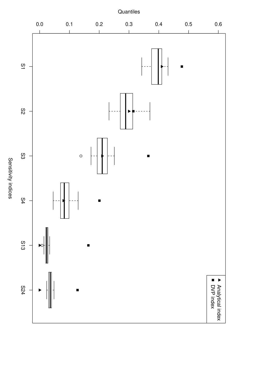
We see that has the biggest contribution, whereas the influence of is very low.
It reflects well the model if we look at the coefficients of , .
Also, interaction terms are well estimated, as they are closed to .
For each case, the dispersion on simulations is very low.
As for the DVP estimation, it is once again very high compared with the true indices values.
5.3 The Ishigami function
This function is well known in SA ([23]). It is defined by:
We assume that is the independent variable, and that and are correlated. is again the Gaussian mixture .
With simulations of observations, we fixed parameters of distribution at , , , and .
In Figure 2, the dispersion of the new measures is represented for fixed and different values of .
In addition, the analytical new indices and estimated classical Sobol indices with DVP are displayed.

Every boxplot shows that there is a small dispersion.
For all estimations, DVP indices are larger that the new ones.
The figure clearly shows that, for all values of , the sum of these four indices is greater
than . It again shows their non adaptation to a situation of dependence.
If we have a look on the values taken by our new sensitivity indices, we see that,
for small values of , the variable contributes the most to the model’s variability.
This role decreases as increases, and then gets the biggest contribution.
For any value of , the input plays a very negligible role, which seems realistic as is a small fixed value.
As for the interaction index , it is getting bigger with the increasing importance of , but the contribution remains low.
6 Conclusions and Perspectives
The Hoeffding decomposition and associated Sobol indices have been widely studied in SA over past years.
Recently, a literature appears to treat the case of dependent input variables, in which authors propose different ways to deal with dependence.
The goal of this paper is to conciliate the problem of inputs dependence with the Hoeffding decomposition.
Indeed, we study a functional ANOVA decomposition in a generalized inputs distribution frame.
Thus, we show that a model can be uniquely decomposed as a sum of hierarchically orthogonal functions of increasing dimension.
Also, this approach generalizes the Hoeffding’s one, as we recover it in case of independence.
Similarly to the classical Sobol decomposition, this leads to the construction of new sensitivity indices.
They consist of a variance and a covariance contribution able to take into account the possible correlation among variables.
In case of independence, these indices are the classical Sobol indices.
However, the indices construction is only possible under specific assumptions on the joint distribution function of the inputs.
We expose few cases that satisfy these assumptions for any -dimensional models.
More specifically, for two-dimensional models, the required assumption is equivalent to assumptions on copulas.
In this context, we give examples satisfying one of these assumptions .
Focused on the IPDV models, summands of the decomposition are estimated thanks to projection operations.
This leads to the numerical resolution of functional linear systems.
The strength of this method is that it does not require to make assumptions on the form of the model or on the structure of dependence. We neither use meta-modelling and avoid in this way many sources of errors.
Through three applications on test models, we observe the importance of considering the inputs correlation, and show how our method could catch it.
The comparison with estimators of classical indices with DVP shows that the Sobol indices are not appropriate in case of correlations, even when using nonparametric method.
Also, when inputs independence holds, the new indices remain well suited to measure sensitivity into a model.
Nevertheless, only considering IPDV models for estimation is restrictive.
The perspective is to explore other estimation methods suitable for more general models.
Also, we intend to lead a systematic study on copulas satisfying or not our assumptions.
A Generalized Hoeffding decomposition
A.1 Generalized decomposition for dependent inputs
The upcoming proof follows the guideline of the proof of Lemma 3.1 in Stone [28].
Proof of Lemma 1
By induction on the cardinal of , let show that
- •
is obviously true, as is reduced to a singleton
- •
Let . Suppose that is true for all . Let such that . We want to prove .
Choose a maximal set of , i.e. is not a proper subset of any set in . We show first that
(28) - –
If , by definition of , we get as .
- –
If , set , where and . By Condition (2.3), it follows that
As a consequence,
By maximality of and by definition of ,
- *
If , only depends on and by orthogonality,
- *
If , depends on fixed at , and , so , with , it comes then
Thus,
- *
So (28) holds for any size of any maximal sets of .
By using (28) with and , , we get
(29) Taking , it follows that:
Hence,
(30) This implies
(31) Set .(31) is rephrased as
(32) As is supposed to be true and (31) holds, it follows that:
Hence, holds.
- –
We can deduce that is true for any collection of .
Proof of Theorem 1
Let define the vector space .
In the first step, we will prove that is a complete space to prove the existence and uniqueness of the projection of in ,
thanks to the projection theorem [16].
Secondly, we will show that is exactly equal to the decomposition into , and finally, we will see that each term of the summand
is unique.
- •
We show that is closed into (as is a Hilbert space).
Let be a convergent sequence of with . As complete, . Let , and :
Thus, , so that . is then a complete space.
Let be a Cauchy sequence in and we show that each component is of Cauchy and that .
As , , . It follows that :
As is a Cauchy sequence, by the above inequality, is also Cauchy. As , we deduce that .
Thus, is complete. By the projection theorem, we can deduce there exists a unique element into such that :
- •
Decomposition of : following Hooker [10], we introduce the residual term as
By projection, , . Hence, , , , and this decomposition is well defined.
- •
Terms of the summand are unique: assume that .
By Lemma 1, it follows that
Proof of Proposition 1
Let first prove the following equivalence :
Let and , then
Conversely, assume that such that , then,
and
There is a contradiction, so that .
The second expression can be rewritten as :
Then, by Theorem 1, the minimization problem admits a unique solution.
A.2 Generalized sensitivity indices
Proof of Proposition 2
with , . Therefore,
and
B Examples of distribution function
B.1 Boundedness of the inputs density function
Proof of Proposition 3
Let , and . As and are marginals, they are upper bounded by .
As a consequence, , so that , with .
Proof of Example 3.1
- •
is a product of measure as , with . So
- •
is given by
(33) First, we have .
Further, the sufficient and necessary condition to have is to get positive definite. Indeed, if admits a negative eigenvalue, can not be bounded. Thus, iff is positive definite.
B.2 Examples of distribution of two inputs
Proof of Proposition 4
If (3) holds, then . Conversely, we assume that , and
It is enough to show it is a copula : Obviously, and . By second order derivation, it comes that , so by hypothesis (2).
C Estimation
C.1 Model of input variables
Proof of Proposition 7
- •
We first show first that () admits an unique solution.
with
Thus,
(34) So is solution of ().
Now, assume there exists an another solution of the system, say , then
As and , it follows that
As can be uniquely decomposed into as a sum of zero, then,
- •
Let now compute
First of all, it is obvious that the constant term and that is obtained by subtracting with all other terms of the right of the decomposition.
Now, let us use the projector’s property of embedded spaces. Indeed, as , , it comes
is a function of , so it can be decomposed into the following expression :
with .
Hence, one can easily deduce , , as the termWe obtain
(35)
C.2 Numerical procedure
Gauss-Seidel algorithm requires the estimation of conditional expectation at each iteration.
To do this, we use the local polynomial estimation with a leave-one-out technique.
To considerably reduce time cost in application, the Sherman-Morrison formula is exploited.
We are going to review these methods for estimating , when and are supposed to be real random variable.
The local polynomial estimation [8] consists in approximating by a -order polynomial fitted by a weight least squared estimation.
An explicit solution of is given by :
| (36) |
with
The leave-one-out technique on local estimation consists in estimating in every observation point , i.e. computing Equation (36) when the line of matrices has been removed for estimating . It means that we would need to inverse times, which is very expensive. To avoid these expensive computations, Sherman and Morrison [24] proposed a formula :
Lemma 2.
If is a square invertible matrix, and , are vectors such that , then
| (37) |
In our problem, set . can be rewritten as :
| (38) |
where
Thus, , corresponding to when the line has been removed, is of the form :
The Sherman-Morrison formula gives :
| (39) |
As , , it is faster to estimate and at each point of the design.
Acknowledgement
This work has been supported by French National Research Agency (ANR) through COSINUS program (project COSTA-BRAVA number ANR-09-COSI-015).
References
- [1] [author] Borgonovo, E.E. (2007). A new uncertainty importance measure. Reliability Engineering and System Safety 92 771-784.
- [2] [author] Borgonovo, E.E., Castaings, W.W. and Tarantola, S.S. (2011). Moment Independent Importance Measures: New Results and Analytical Test Cases. Risk Analysis 31 404-428.
- [3] [author] Cukier, R. I.R. I., Schaibly, J. H.J. H. and Shuler, K. E.K. E. (1975). Study of the sensitivity of coupled reaction systems to uncertainties in rate coefficients. III. Analysis of the approximations. Journal of Chemical physics 63 431-440.
- [4] [author] Cukier, R. I.R. I., Levine, H. B.H. B. and Shuler, K. E.K. E. (1978). Nonlinear sensitivity analysis of multiparameter model systems. The Journal of Computational Physics 26 1-42.
- [5] [author] Da Veiga, S.S. (2007). Analyse d’incertitudes et de sensibilité Application aux modèles de cinétique chimique PhD thesis, Université Toulouse III.
- [6] [author] Da Veiga, S.S., Wahl, F.F. and Gamboa, F.F. (2009). Local Polynomial Estimation for Sensitivity Analysis on Models With Correlated Inputs. Technometrics 51 452-463.
- [7] [author] De Pillis, J.J. (1973). Gauss-Seidel convergence for operators on Hilbert space. SIAM Journal of Numerical Analysis 10 112-122.
- [8] [author] Fan, J.J. and Gijbels, I.I. (1996). Local polynomial modelling and its application. Chapman & Hall, London.
- [9] [author] Hoeffding, W.W. (1948). A class of statistics with asymptotically normal distribution. The annals of Mathematical Statistics 19 293-325.
- [10] [author] Hooker, G.G. (2007). Generalized functional ANOVA diagnostics for high-dimensional functions of dependent variables. Journal of Computational and Graphical Statistics 16 709-732.
- [11] [author] Jacques, J.J., Lavergne, C.C. and Devictor, N.N. (2006). Sensitivity analysis in presence of model uncertainty and correlated inputs. Reliability Engineering and System Safety 91 1126-1134.
- [12] [author] Jensen, J. L.J. L. (1906). Sur les fonctions convexes et les inégalités entre les valeurs moyennes. Acta Mathematica 10 175-193.
- [13] [author] Kress, R.R. (1998). Numerical analysis. Springer, New York.
- [14] [author] Li, G.G., Rabitz, H.H., Hu, J.J., Chen, Z.Z. and Ju, Y.Y. (2008). Regularized random-sampling high dimensional model representation. Journal of Mathematical Chemistry 43 6022-6032.
- [15] [author] Li, G.G., Rabitz, H.H., Yelvington, P. E.P. E., Oluwole, O.O., Bacon, F.F., E., Kolb C.K. C. and Schoendorf, J.J. (2010). Global sensitivity analysis with independent and/or correlated inputs. Journal of Physical Chemistry A 114 6022-6032.
- [16] [author] Luenberger, D. G.D. G. Optimization by vector space methods. Wiley, New York.
- [17] [author] Mara, T.T. and Tarantola, S.S. (2012). Variance-based sensitivity analysis of computer models with dependent inputs. Reliability Engineering and System Safety.
- [18] [author] Morgenstern, D.D. (1956). Einfache Beispiele Zweidimensionaler Verteilungen. Mitteilingsblatt fur Mathematische Statistik 8 234-253.
- [19] [author] Nelsen, R. B.R. B. An introduction to copulas. Springer, New York.
- [20] [author] Ouyang, Z.Z., Liao, H.H. and Yang, X.X. (2009). Modeling dependence based on mixture copulas and its application in risk management. Appl. Math. J. Chinese Univ. 24 393-401.
- [21] [author] Owen, A. B.A. B. (1994). Lattice sampling revisited:Monte Carlo variance of means over randomized orthogonal arrays. The Annals of Statistics 22 930-945.
- [22] Owen, A. B. (2005). Multidimensional variation for quasi-Monte Carlo. In International Conference on Statistics in honour of Professor Kai-Tai Fang’s 65th birthday (J. Fan and G. Li, eds.) 49–74.
- [23] [author] Saltelli, A.A., Chan, K.K. and Scott, E. M.E. M. (2000). Sensitivity Analysis. Wiley, West Sussex.
- [24] [author] Sherman, J.J. and Morrison, W. J.W. J. (1950). Adjustment of an Inverse Matrix Corresponding to a Change in One Element of a Given Matrix. The Annals of Mathematical Statistics 21 124-127.
- [25] [author] Sklar, A.A. (1971). Random Variables, Joint Distribution Functions, and Copulas. Kybernetika 9 449-460.
- [26] [author] Sobol, I. M.I. M. (1993). Sensitivity estimates for nonlinear mathematical models. Wiley 1 407-414.
- [27] [author] Sobol, I. M.I. M. (2001). Global sensitivity indices for nonlinear mathematical models and their Monte Carlo estimates. Mathematics and Computers in Simulations 55.
- [28] [author] Stone, C. J.C. J. (1994). The use of Polynomial Splines and their tensor products in multivariate function estimation. The Annals of Statistics 22 118-171.
- [29] [author] Tarantola, S.S., Gatelli, D.D. and Mara, T.T. (2006). Random Balance Designs for the Estimation of First Order Global Sensitivity Indices. Reliability Engineering and System Safety 91 717-727.
- [30] [author] Tissot, J. Y.J. Y. and Prieur, C.C. (2011). A bias correction method for the estimation of sensitivity indices based on random balance designs. Submitted http://hal.archives-ouvertes.fr/hal-00507526/fr/.
- [31] [author] Van Der Vaart, A. W.A. W. Asymptotic Statistics. Cambridge University Press, Cambridge.
- [32] [author] Xu, C.C. and Gertner, G.G. (2008). Uncertainty and sensitivity analysis for models with correlated parameters. Reliability Engineering and System Safety 93 1563-1573.