Heegard-Berger and Cascade Source Coding Problems with Common Reconstruction Constraints

In applications such as the ones discussed above, the point-to-point setting of Fig. 1 does not fully capture the main features of the source coding problem. For instance, in video streaming, a transmitter typically broadcasts information to a number of decoders. As another example, in sensor networks, data is typically routed over multiple hops towards the destination. A model that accounts for the aspect of broadcasting to multiple decoders is the Heegard-Berger (HB) set-up shown in Fig. 2. In this model, the link of rate $R$ bits per source symbol is used to communicate to two receivers having different side information sequences, $Y_{1}^{n}$ and $Y_{2}^{n}$, which are related to source $X^{n}$ via a memoryless channel $p(y_{1},y_{2}|x)$. The set of all achievable triples ($R,D_{1},D_{2}$) for this model, where $D_{1}$ and $D_{2}$ are the distortion levels at Decoders 1 and 2 respectively, was derived in [6] and [7] under the assumption that the side information sequences are (stochastically) degraded versions of the source $X^{n}$. In a variation of this model shown in Fig. 3, decoder cooperation is enabled by a limited capacity link from one decoder (Decoder 1) to the other (Decoder 2). Inner and outer bounds to the rate distortion region for this problem are obtained in [8] under the assumption that the side information of Decoder 2 is (physically) degraded with respect to that of Decoder 1.

As for multihopping, a basic model that captures some of the key design issues is shown in Fig. 4. In this cascade set-up, an encoder (Node 1) communicates with rate $R_{1}$ to a intermediate node (Node 2), which has side information $Y_{1}^{n}$, and in turns communicates with rate $R_{2}$ to a final node (Node 3) with side information $Y_{2}^{n}$. Both Node 2 and Node 3 act as decoders, similar to the HB problem of Fig. 2, in the sense that they reconstruct a local estimate of the source $X^{n}$. The rate-distortion function for this problem has been derived for various special cases in [9, 10, 11] and [12] (see Table I in [12] for an overview). Reference [11] derives the set of all achievable quadruples $(R_{1},R_{2},D_{1},D_{2})$, i.e., the rate-distortion region, for the case in which $Y_{1}^{n}$ is also available at the encoder and $Y_{2}^{n}$ is a physically degraded version of $X^{n}$ with respect to $Y_{1}^{n}$. Instead, [10] derives the rate-distortion region under the assumptions that the source and the side information sequences are jointly Gaussian, that the distortion metric is quadratic, and that the sequence $Y_{1}^{n}$ is a physically degraded version of $X^{n}$ with respect to $Y_{2}^{n}$. The corresponding result for binary source and side information and Hamming distortion metric was derived in [12].

A key aspect of the optimal strategies identified in [4, 6, 7, 10] and [11] is that the side information sequences are, in general, used in two different ways: (i) as a means to reduce the rate required for communication between encoder and decoders via binning; and (ii) as an additional observation that the decoder can leverage, along with the bits received from the encoder, in order to improve its local estimate. For instance, for the point-to-point system of Fig. 1, the Wyner-Ziv result (1) reflects point (i) of the discussion above in the conditioning on side information $Y$, which reduces the rate, and point (ii) in the fact that the reconstruction $\hat{X}$ is a function $\mathrm{\hat{x}}(U,Y)$ of the signal $U$ received from the encoder and the side information $Y$.

Leveraging the side information as per point (ii), while advantageous in terms of rate-distortion trade-off, may have unacceptable consequences for some applications. In fact, this use of side information entails that the reconstruction $\hat{X}$ of the decoder cannot be reproduced at the encoder. In other words, encoder and decoder cannot agree on the specific reconstruction $\hat{X}$ obtained at the receiver side, but only on the average distortion level $D$. In applications such as transmission of sensitive medical, military or financial data, this may not be desirable. Instead, one may want to add the constraint that the reconstruction at the decoder be reproducible by the encoder [5]. This idea, referred to as the Common Reconstruction (CR) constraint, was first proposed in [5], where it is shown for the point-to-point setting of Fig. 1²² 2 The function $\psi$ at the encoder calculates the estimate of the encoder regarding the decoder’s reconstruction. that the rate-distortion function under the CR constraint is given by

where the minimum is taken over all pmfs $p(\hat{x}|x)$ such that $\mbox{E}[d(X,\hat{X})]\leq D$. Comparing (2) with the Wyner-Ziv rate-distortion (1), it can be seen that the additional CR constraint prevents the decoder from using the side information as a means to improve its estimate $\hat{X}$ (see point (ii) above).

The original work of [5] has been recently extended in [13], where a relaxed CR constraint is imposed in which only a distortion constraint is imposed between the decoder’s reconstruction and its reproduction at the encoder. We refer to this setting as imposing a Constrained Reconstruction (ConR) requirement.

In this paper, we study the HB source coding problem (Fig. 2) and the cascade source coding problem (Fig. 4) under the CR requirement. The considered models are thus relevant for the transmission of sensitive information, which is constrained by CR, via broadcast or multi-hop links – a common occurrence in, e.g., medical, military or financial applications (e.g., for intranets of hospitals or financial institutions). Specifically, our main contributions are:

• •

  For the HB problem with the CR constraint (Fig. 2), we derive the rate-distortion function under the assumption that the side information sequences are (stochastically) degraded. We also calculate this function explicitly for three examples, namely Gaussian source and side information with quadratic distortion metric, and binary source and erasure side information with erasure and Hamming distortion metrics (Sec. II);

• •

  For the HB problem with the CR constraint and decoder cooperation (Fig. 3), we derive the rate-distortion region under the assumption that the side information sequences are (physically) degraded in either direction (Sec. III-A and Sec. III-B). We emphasize that the corresponding problem without the CR constraint is still open as per the discussion above;

• •

  For the cascade problem with the CR constraint (Fig. 4), we obtain the rate-distortion region under the assumption that side information $Y_{2}$ is physically degraded with respect to $Y_{1}$ (Sec. IV-B). We emphasize that the corresponding problem without the CR constraint is still open as per the discussion above;

• •

  For the cascade problem with CR constraint (Fig. 4), we obtain outer and inner bounds on the rate-distortion region under the assumption that the side information $Y_{1}$ is physically degraded with respect to $Y_{2}$. Moreover, for the three examples mentioned above in the context of the HB problem, we show that the bounds coincide and we evaluate the corresponding rate-distortion region explicitly (Sec. IV-C);

• •

  For the HB problem, we finally derive the rate-distortion function under the more general requirement of ConR (Sec. V).

Notation: For $a$ and $b$ integer with $a\leq b$ we define $[a,b]$ as the interval $[a,a+1,...,b]$ and we use $x_{a}^{b}$ to denote the sequence $(x_{a},\ldots,x_{b})$. We will also write $x^{b}$ for $x_{1}^{b}$ for simplicity. Upper case, lower case and calligraphic letters denote random variables, specific values of random variables and their alphabets, respectively. Given discrete random variables, or more generally vectors, $X$ and $Y$, we will use the notation $p_{X}(x)$ or $p(x)$ for ${}\mathrm{Pr}[X=x]$, and $p_{X|Y}(x|y)$ or $p(x|y)$ for ${}\mathrm{Pr}[X=x|Y=y]$, where the latter notations are used when the meaning is clear from the context. Given a set $\mathcal{X}$, we denoted by $\mathcal{X}^{n}$ the $n$-fold Cartesian product of $\mathcal{X}$. For random variables $X$ and $Y$, we denote by $\sigma_{X|Y}^{2}$ the (average) conditional variance of $X$ given $Y$, i.e., $\textrm{E}\left[\textrm{E}[(X-\textrm{E}[X|Y])^{2}|Y]\right].$ We adopt the notation convention in [14], in which $\delta(\epsilon)$ represents any function such that $\delta(\epsilon)\rightarrow 0$ as $\epsilon\rightarrow 0$. We define the binary entropy function $H(p)=-p\textrm{lo$g_{2}$}p-(1-p)\textrm{lo$g_{2}$}(1-p)$. Finally, we define $\alpha*\beta=\alpha(1-\beta)+\beta(1-\alpha)$.

In this section the system model for the HB problem with CR is detailed. The system is defined by the pmf $p_{XY_{1}Y_{2}}(x,y_{1},y_{2})$ and discrete alphabets $\mathcal{X},\mathcal{Y}_{1},\mathcal{Y}_{2},\hat{\mathcal{X}}_{1},$ and $\hat{\mathcal{X}}_{2}$ as follows. The source sequence $X^{n}$ and side information sequences $Y_{1}^{n}$ and $Y_{2}^{n}$, with $X^{n}\in\mathcal{X}^{n}$, $Y_{1}^{n}\in\mathcal{Y}_{1}^{n}$, and $Y_{2}^{n}\in\mathcal{Y}_{2}^{n}$ are such that the tuples $(X_{i},Y_{1i},Y_{2i})$ for $i\in[1,n]$ are independent and identically distributed (i.i.d.) with joint pmf $p_{XY_{1}Y_{2}}(x,y_{1},y_{2})$. The encoder measures a sequence $X^{n}$ and encodes it into a message $J$ of $nR$ bits, which is delivered to the decoders. Decoders 1 and 2 wish to reconstruct the source sequence $X^{n}$ within given distortion requirements, to be discussed below, as $\hat{X}_{1}^{n}\in\mathcal{\hat{X}}_{1}^{n}$ and $\hat{X}_{2}^{n}\in\mathcal{\hat{X}}_{2}^{n}$, respectively. The estimated sequence $\hat{X}_{j}^{n}$ is obtained as a function of the message $J$ and the side information sequence $Y_{j}^{n}$ for $j=1,2$. The estimates are constrained to satisfy distortion constraints defined by per-symbol distortion metrics $d_{j}(x,\hat{x}_{j}):\mathcal{X}\times\mathcal{\hat{X}}_{j}\rightarrow[0,D_{max}]$ with $0<D_{max}<\infty$. Based on the given distortion metrics, the overall distortion for the estimated sequences $\hat{x}_{1}^{n}$ and $\hat{x}_{2}^{n}$ is defined as

The reconstructions $\hat{X}_{2}^{n}$ and $\hat{X}_{2}^{n}$ are also required to satisfy the CR constraints, as formalized below.

In this section, a single-letter characterization of the rate-distortion function for the HB problem with CR is derived, under the assumption that the joint pmf $p(x,y_{1},y_{2})$ is such that there exists a conditional pmf $\tilde{p}(y_{1}|y_{2})$ for which

In other words, the side information $Y_{1}$ is a stochastically degraded version of $Y_{2}.$

The proof of the converse can be found in Appendix A. Achievability follows as a special case of Theorem 3 of [6] and can be easily shown using standard arguments. In particular, the encoder randomly generates a standard lossy source code $\hat{X}_{1}^{n}$ for the source $X^{n}$ with rate $I(X;\hat{X}_{1})$ bits per source symbol. Random binning is used to reduce the rate to $I(X;\hat{X}_{1}|Y_{1}).$ By the Wyner-Ziv theorem [14, p. 280], this guarantees that both Decoder 1 and Decoder 2 are able to recover $\hat{X}_{1}^{n}$ (since $Y_{1}$ is a degraded version of $Y_{2}$). The encoder then maps the source $X^{n}$ into the reconstruction sequence $\hat{X}_{2}^{n}$ using a codebook that is generated conditional on $\hat{X}_{1}^{n}$ with rate $I(X;\hat{X}_{2}|\hat{X}_{1})$ bits per source symbol. Random binning is again used to reduce the rate to $I(X;\hat{X}_{2}|Y_{2}\hat{X}_{1})$. From the Wyner-Ziv theorem, and the fact that Decoder 2 knows the sequence $\hat{X}_{1}^{n}$, it follows that Decoder 2 can recover the reconstruction $\hat{X}_{2}^{n}$ as well. Note that, since the reconstruction sequences $\hat{X}_{1}^{n}$ and $\hat{X}_{2}^{n}$ are generated by the encoder, functions $\psi_{1}$ and $\psi_{2}$ that guarantees the CR constraints (9) exist by construction.

In this section, we highlight the result of Proposition 2 by considering a zero-mean Gaussian source $X\sim\mathcal{N}(0,\sigma_{x}^{2})$, with side information variables

where $Z_{1}\sim\mathcal{N}(0,N_{1}+N_{2})$ and $Z_{2}\sim\mathcal{N}(0,N_{2})$ are independent of each other and of $Y_{2}$ and $X$. Note that the joint distribution of $(X,Y_{1},Y_{2})$ satisfies the stochastic degradedness condition. We focus on the quadratic distortion $d_{j}(x,\hat{x}_{j})=(x-\hat{x}_{j})^{2}$ for $j=1,2$. By leveraging standard

arguments that allow us to apply Proposition 2 to Gaussian sources under mean-square-error constraint (see [14, pp. 50-51] and [15]), we obtain a characterization of the rate-distortion function for the given distortion and metrics.

We first recall that for the point-to-point set-up in Fig. 1 with $X\sim\mathcal{N}(0,\sigma_{x}^{2})$ and side information $Y=X+Z,$ with $Z\sim\mathcal{N}(0,N)$ independent of $X,$ the rate-distortion function with CR under quadratic distortion is given by [5]

where we have made explicit dependence on $N$ of function $R_{\mathcal{G}}^{\mathcal{\mbox{$CR$}}}(D,N)$ for convenience. The rate-distortion function (II-C) for $D\leq\sigma_{x}^{2}$ is obtained from (2) by choosing the distribution $p(\hat{x}|x)$ such that $X=\hat{X}+Q$ where $Q\sim\mathcal{N}(0,D)$ is independent of $\hat{X}$.

Definition of the rate distortion function (7) requires different consideration for the four subregions of the $(D_{1},D_{2})$ plane sketched in Fig. 5. In fact, for $D_{1}\geq\sigma_{x}^{2}\mbox{ and }D_{2}\geq\sigma_{x}^{2}$, the required rate is zero, since the distortion constraints are trivially met by setting $\hat{X_{1}}=\hat{X_{2}}=0$ in the achievable rate (11). For the case $D_{1}\geq\sigma_{x}^{2}\mbox{ and }D_{2}\leq\sigma_{x}^{2}$, it is sufficient to cater only to Decoder 2 by setting $\hat{X_{1}}=0$ and $X=\hat{X}_{2}+Q_{2}$, with $Q_{2}\sim\mathcal{N}(0,D_{2})$ independent of $\hat{X_{2}}$, in the achievable rate (11). That this rate cannot be improved upon follows from the trivial converse

which follows by cut-set arguments. The same converse suffices also for the regime $D_{1}\leq\sigma_{x}^{2}\mbox{ and }D_{2}\geq\min(D_{1},\sigma_{x}^{2})$. For this case, achievability follows by setting $X=\hat{X}_{1}+Q_{1}$ and $\hat{X_{1}}=\hat{X_{2}}$ in (11), where $Q_{1}\sim\mathcal{N}(0,D_{1})$ is independent of $\hat{X_{1}}$. In the remaining case, namely $D_{2}\leq D_{1}\leq\sigma_{x}^{2}$, the rate-distortion function does not follow from the point-to-point result (II-C) as for the regimes discussed thus far. The analysis of this case requires use of entropy-power inequality (EPI) and can be found in Appendix B

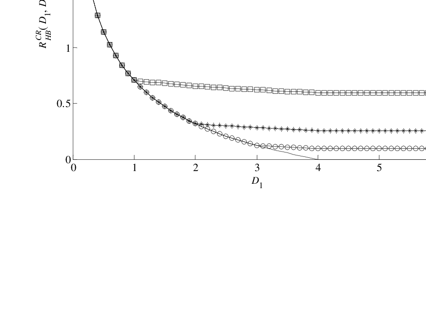
Fig. 6 depicts the rate $R_{HB}^{CR}(D_{1},D_{2})$ in (7) versus $D_{1}$ for different values of $D_{2}$ with $\sigma_{x}^{2}=4$, $N_{1}=2$, and $N_{2}=3.$ As discussed above, for $D_{2}=5$, which is larger than $\sigma_{x}^{2}$, $R_{HB}^{CR}(D_{1},D_{2})$ becomes zero for values of $D_{1}$ larger than $\sigma_{x}^{2}=4$, while this is not the case for values $D_{2}<\sigma_{x}^{2}=4$.

In this section, we consider a binary source $X\sim\textrm{Ber}(\frac{1}{2})$ with erased side information sequences $Y_{1}$ and $Y_{2}$. The source $Y_{2}$ is an erased version of the source $X$ with erasure probability $p_{2}$ and $Y_{1}$ is an erased version of $X$ with erasure probability $p_{1}>p_{2}.$ This means that $Y_{j}=e$, where $e$ represents an erasure, with probability $p_{j}$ and $Y_{j}=X$ with probability $1-p_{j}$. Note that, with these assumptions, the side information $Y_{1}$ is stochastically degraded with respect to $Y_{2}.$ In fact, we have the factorization (10), where additional distributions $p(y_{2}|x)$ and $\tilde{p}(y_{1}|y_{2})$ are illustrated in Fig. 7. As seen in Fig. 7, the pmf $\tilde{p}(y_{1}|y_{2})$ is characterized by the probability $\tilde{p}_{1}$ that satisfies the equality $p_{1}=p_{2}+\tilde{p}_{1}(1-p_{2})$. We focus on Hamming and erasure distortions. For the Hamming distortion, the reconstruction alphabets are binary, $\hat{\mathcal{X}}_{1}=\hat{\mathcal{X}}_{2}=\{0,1\}$, and we have $d_{j}(x,\hat{x}_{j})=0$ if $x=\hat{x}_{j}$ and $d_{j}(x,\hat{x}_{j})=1$ otherwise for $j=1,2$. Instead, for the erasure distortion the reconstruction alphabets are $\hat{\mathcal{X}}_{1}=\hat{\mathcal{X}}_{2}=\{0,1,e\}$, and we have for $j=1,2$:

In Appendix C, we prove that for the point-to-point set-up in Fig. 1 with $X\sim\textrm{Ber}(\frac{1}{2})$ and erased side information $Y,$ with erasure probability $p$, the rate-distortion function with CR under Hamming distortion is given by

where we have made explicit the dependence on $p$ of function $R_{\mathcal{B}}^{CR}(D,p)$ for convenience. The rate-distortion function (II-D) for $D\leq 1/2$ is obtained from (2) by choosing the distribution $p(\hat{x}|x)$ such that $X=\hat{X}\oplus Q$ where $Q\sim\textrm{Ber}(D)$ is independent of $\hat{X}$. Following the same steps as in Appendix C, it can be also proved that for the point-to-point set-up in Fig. 1 with $X\sim\textrm{Ber}(\frac{1}{2})$ and erased side information $Y,$ with erasure probability $p$, the rate-distortion function with CR under erasure distortion is given by

The rate-distortion function (33) is obtained from (2) by choosing the distribution $p(\hat{x}|x)$ such that $\hat{X}=X$ with probability $1-D$ and $\hat{X}=e$ with probability $D$.

Similar to the Gaussian example, the characterization of the rate distortion function (10) requires different considerations for the four subregions of the $(D_{1},D_{2})$ plane sketched in Fig. 8. In fact, for $D_{1}\geq 1/2\mbox{ and }D_{2}\geq 1/2$, the required rate is zero, since the distortion constraints are trivially met by setting $\hat{X_{1}}=\hat{X_{2}}=0$ in the achievable rate (11). For the case $D_{1}\geq 1/2\mbox{ and }D_{2}\leq 1/2$, it is sufficient to cater only to Decoder 2 by setting $\hat{X_{1}}=0$ and $X=\hat{X}_{2}\oplus Q_{2}$, with $Q_{2}\sim\textrm{Ber}(D_{2})$ independent of $X$, in the achievable rate (11). That this rate cannot be improved upon is a consequence from the trivial converse

which follows by cut-set arguments. The same converse suffices also for the regime $D_{1}\leq 1/2\mbox{ and }D_{2}\geq\min(D_{1},1/2)$. For this case, achievability follows by setting $X=\hat{X}_{1}\oplus Q_{1}$ and $\hat{X_{1}}=\hat{X_{2}}$ in (11), where $Q_{1}\sim\textrm{Ber}(D_{1})$ is independent of $\hat{X}_{1}$. In the remaining case, namely $D_{2}\leq D_{1}\leq 1/2$, the rate-distortion function does not follow from the point-to-point result (II-D) as for the regimes discussed thus far. The analysis of this case can be found in Appendix D. Similar arguments apply also for the erasure distortion metric.

We now compare the rate-distortion function for the binary source $X\sim\textrm{Ber}(\frac{1}{2})$ with erased side information under Hamming distortion for three settings. In the first setting, known as the Kaspi model [7], the encoder knows the side information, and thus the position of the erasures. For this case, the rate-distortion function $R_{Kaspi}(D_{1},D_{2})$ for the example at hand was calculated in [17]. Note that in the Kaspi model, the CR constraint does not affect the rate-distortion performance since the encoder has all the information available at the decoders. The second model of interest is the standard HB setting with no CR constraint, whose rate-distortion function $R_{HB}(D_{1},D_{2})$ for the example at hand was derived [12]. The third model is the HB setup with CR studied here. We clearly have the inequalities

where the first inequality in (42) accounts for the impact of the availability of the side information at the encoder, while the second reflects the potential performance loss due to the CR constraint.

Fig. 9 shows the aforementioned rate-distortion functions with $p_{1}=1$ and $p_{2}=0.35$, which corresponds to the case where Decoder 1 has no side information, for two values of the distortion $D_{2}$ versus the distortion $D_{1}$. For $D_{2}\geq\frac{p_{2}}{2}=0.175$, the given settings reduce to one in which the encoder needs to communicate information only to Decoder 1. Since Decoder 1 has no side information, the Kaspi and HB settings yield equal performance i.e., $R_{Kaspi}(D_{1},D_{2})=R_{HB}(D_{1},D_{2})$.

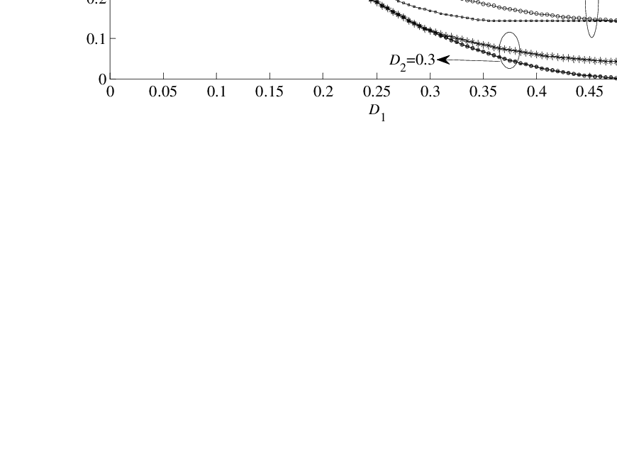
Moreover, if $D_{1}$ is sufficiently smaller than $D_{2}$, the operation of the encoder is limited by the distortion requirements of Decoder 1. In this case, Decoder 2 can in fact reconstruct as $\hat{X}_{1}=\hat{X}_{2}$ while still satisfying its distortion constraints. Therefore, we obtain the same performance in all of the three settings, i.e., $R_{Kaspi}(D_{1},D_{2})=R_{HB}(D_{1},D_{2})=R_{HB}^{CR}(D_{1},D_{2}).$ We also note the general performance loss due to the CR constraint, unless, as discussed above, distortion $D_{1}$ is sufficiently smaller than $D_{2}$.

In this section, a single-letter characterization of the rate-distortion region is derived under the assumption that the joint pmf $p(x,y_{1},y_{2})$ is such that the Markov chain $X-Y_{1}-Y_{2}$ holds³³ 3 Note that, unlike the conventional HB problem studied in Sec. II, the rate-distortion region with cooperative decoders depends on the joint distribution of the variables ($Y_{1},Y_{2}$), and thus stochastic and physical degradedness of the side information sequences lead to different results..

The proof of the converse can be easily established following cut-set arguments for bound (45a), while the bound (45b) on the sum-rate $R_{1}+R_{2}$ can be proved following the same step as in Appendix A and substituting $J$ with $(J_{1},J_{2})$. As for the achievability, it follows as a straightforward extension of [8, Sec. III] to the setup at hand where Decoder 2 has side information as well. It is worth emphasizing that the reconstruction $\hat{X}_{2}$ for the Decoder 2, which has degraded side information, is conveyed by using both the direct link from the Encoder, of rate $R_{1}$, and the path Encoder-Decoder 1-Decoder 2. The latter path leverages the the better side information at Decoder 1 and the cooperative link of rate $R_{2}$.

In this section, a single-letter characterization of the rate-distortion region is derived under the assumption that the joint pmf $p(x,y_{1},y_{2})$ is such that the Markov chain relationship $X-Y_{2}-Y_{1}$ holds.

The proof of achievability follows immediately by neglecting the link of rate $R_{2}$ and using rate $R_{1}$ as per the HB scheme of Proposition 2. The converse follows by considering an enhanced system in which Decoder 2 is provided with the side information of Decoder 1. In this system, link $R_{2}$ becomes useless since Decoder 2 possesses all the information available at Decoder 1. It follows that the system reduces to the HB problem with degraded sources studied in the previous section and the bound (47a) follows immediately from Proposition 2.

In this section, the system model for the cascade source coding problem with CR is detailed similar to Sec. II-A. The problem is defined by the pmf $p_{XY_{1}Y_{2}}(x,y_{1},y_{2})$ and discrete alphabets $\mathcal{X},\mathcal{Y}_{1},\mathcal{Y}_{2},\hat{\mathcal{X}}_{1},$ and $\hat{\mathcal{X}}_{2}$ as follows. The source sequence $X^{n}$ and side information sequences $Y_{1}^{n}$ and $Y_{2}^{n}$, with $X^{n}\in\mathcal{X}^{n}$, $Y_{1}^{n}\in\mathcal{Y}_{1}^{n}$, and $Y_{2}^{n}\in\mathcal{Y}_{2}^{n}$ are such that the tuples $(X_{i},Y_{1i},Y_{2i})$ for $i\in[1,n]$ are i.i.d. with joint pmf $p_{XY_{1}Y_{2}}(x,y_{1},y_{2})$. Node 1 measures a sequence $X^{n}$ and encodes it into a message $J_{1}$ of $nR_{1}$ bits, which is delivered to Node 2. Node 2 estimates a sequence $\hat{X}_{1}^{n}\in\mathcal{\hat{X}}_{1}^{n}$ within given distortion requirements. Node 2 also encodes the message $J_{1}$ received from Node 1 and the sequence $Y_{1}^{n}$ into a message $J_{2}$ of $nR_{2}$ bits, which is delivered to Node 3. Node 3 estimates a sequence $\hat{X}_{2}^{n}\in\mathcal{\hat{X}}_{2}^{n}$ within given distortion requirements. Distortion and CR requirements are defined as in Sec. II-A, leading to the following definition.

References

- [1] A. Aaron, R. Zhang and B. Girod, “Wyner-Ziv coding of motion video,” in Proc. Asilomar Conference on Signals, Systems and Computers, Pacific Grove, CA, Nov. 2002.
- [2] Z. Xiong, A. D. Liveris and S. Cheng, “Distributed source coding for sensor networks,” IEEE Signal Processing Magazine, vol. 21, no. 5, pp. 80- 94, Sept. 2004.
- [3] D. Slepian and J. Wolf, “Noiseless coding of correlated information sources,” IEEE Trans. Inform. Theory, vol. 19, no. 4, pp. 471- 480, Jul. 1973.
- [4] A. Wyner and J. Ziv, “The rate-distortion function for source coding with side information at the decoder,” IEEE Trans. Inform. Theory, vol. 22, no. 1, pp. 1- 10, Jan. 1976.
- [5] Y. Steinberg, “Coding and common reconstruction,” IEEE Trans. Inform. Theory, vol. 55, no. 11, 2009.
- [6] C. Heegard and T. Berger, “Rate distortion when side information may be absent,” IEEE Trans. Inform. Theory, vol. 31, no. 6, pp. 727–734, Nov. 1985.
- [7] A. H. Kaspi, “Rate-distortion function when side-information may be present at the decoder,” IEEE Trans. Inform. Theory, vol. 40, pp. 2031–2034, Nov. 1994.
- [8] D. Vasudevan, “On the Heegard-Berger/Kaspi problem with decoder cooperation,” in Proc. IEEE Int’l Conf. on Telecommunications, St. Petersburg, Russia, June 2008.
- [9] H. Yamamoto, “Source coding theory for cascade and branching communication systems,” IEEE Trans. Inform. Theory, vol. 27, no. 3, pp. 299–308, May 1981.
- [10] D. Vasudevan, C. Tian, and S. N. Diggavi, “Lossy source coding for a cascade communication system with side-informations,” In Proc. 44th Annual Allerton Conference on Communications, Control and Computing, Monticello, IL, September 2006.
- [11] Y. K. Chia, H. Permuter and T. Weissman, “Cascade, triangular and two way source coding with degraded side information at the second user,” submitted [http://arxiv.org/abs/1010.3726].
- [12] R. Tandon, S. Mohajer, and H. V. Poor, “Cascade source coding with erased side information,” in Proc. IEEE Symp. Inform. Theory, St. Petersburg, Russia, Aug. 2011.
- [13] A. Lapidoth, A. Malar, and M. Wigger, “Constrained Wyner-Ziv coding,” in Proc. IEEE Symp. Inform. Theory, St. Petersburg, Russia, Aug. 2011.
- [14] A. El Gamal and Y. Kim, Network Information Theory, Cambridge University Press, Dec 2011.
- [15] A. D. Wyner, “The rate-distortion function for source coding with side information at the decoder—II: General sources,” Inform. Contr., vol. 38, pp. 60–80, Jul. 1978.
- [16] T. Weissman and A. El Gamal, “Source coding with limited-look-ahead side information at the decoder," IEEE Trans. Inform. Theory, vol. 52, no. 12, pp. 5218-5239, Dec. 2006.
- [17] E. Perron, S. N. Diggavi, and E. Telatar, “Lossy source coding with Gaussian or erased side-information,” in Proc. IEEE Symp. Inform. Theory, Seoul, South Korea, Jun. 28-July 3, 2009.
- [18] T. Weissman and S. Verdú. “The information lost in erasures,” IEEE Trans. Inform. Theory, vol. 54, no. 11, pp. 5030 – 5058, Nov. 2008.
- [19] R. Timo, A. Grant and G. Kramer, “Rate-distortion functions for source coding with complementary side information,” in Proc. IEEE Symp. Inform. Theory, St. Petersburg, Russia, Aug. 2011.
- [20] P. Cuff, H.-I. Su and A. El Gamal, “Cascade multiterminal source coding,” in Proc. IEEE Int. Symp. Inform. Theory, Seoul, South Korea, Jun. 28-July 3, 2009.
- [21] D. P. Bertsekas, Nonlinear Programming, Athena Scientific, 1999.