On the relativistic precession and oscillation frequencies of test particles around rapidly rotating compact stars
Abstract
Whether analytic exact vacuum(electrovacuum) solutions of the Einstein(Einstein-Maxwell) field equations can accurately describe or not the exterior spacetime of compact stars remains still an interesting open question in Relativistic Astrophysics. As an attempt to establish their level of accuracy, the radii of the Innermost Stable Circular Orbits (ISCOs) of test particles given by analytic exterior spacetime geometries have been compared with the ones given by numerical solutions for neutron stars (NSs) obeying a realistic equation of state (EoS). It has been so shown that the six-parametric solution of Pachón, Rueda, and Sanabria (2006) (hereafter PRS) is more accurate to describe the NS ISCO radii than other analytic models. We propose here an additional test of accuracy for analytic exterior geometries based on the comparison of orbital frequencies of neutral test particles. We compute the Keplerian, frame-dragging, as well as the precession and oscillation frequencies of the radial and vertical motions of neutral test particles for the Kerr and PRS geometries; then we compare them with the numerical values obtained by Morsink and Stella (1999) for realistic NSs. We identify the role of high-order multipole moments such as the mass quadrupole and current octupole in the determination of the orbital frequencies especially in the rapid rotation regime. The results of this work are relevant to cast a separatrix between black hole (BH) and NS signatures as well as probe the nuclear matter EoS and NS parameters from the Quasi-Periodic Oscillations (QPOs) observed in Low Mass X-Ray Binaries.
Subject headings
Exact solutions Einstein-Maxwell equations – Relativistic precession frequenciesI. Introduction
One of the greatest challenges of the general theory of relativity has been the construction of solutions to the Einstein-Maxwell field equations representing the gravitational field of compact stars such as neutron stars (NSs). Stationary axially symmetric spacetimes satisfy basic properties one expects for rotating objects, namely time symmetry and reflection symmetry with respect to the rotation axis (Pachón and Sanabria-Gómez 2006, see e.g.). The simplest stationary axially symmetric exact exterior vacuum solution describing a rotating configuration is the well-known Kerr metric (Kerr 1963). The Kerr metric is fully described by two free parameters: the mass and the angular momentum of the object. However, it is known from numerical models that the quadrupole moment of rotating NSs deviates considerably from the one given by the Kerr solution (see e.g. Laarakkers and Poisson 1999, for details).
In the mean time, a considerable number of analytic exterior solutions with a more complex multipolar structure than the one of the Kerr solution have been developed (Manko et al. 1995; Manko et al. 2000; Stephani et al. 2003, see e.g.). Whether analytic exterior solutions are accurate or not to describe the gravitational field of compact stars is an interesting and very active topic of research (see e.g. Stute and Camenzind 2002; Berti and Stergioulas 2004; Pachón et al. 2006, and references therein).
The accuracy of analytic solutions to describe the exterior geometry of a realistic rotating compact star has been tested by comparing physical properties, e.g. the radius of the Innermost Stable Circular Orbit (ISCO) on the equatorial plane and the gravitational redshift (see Sibgatullin and Sunyaev 1998; Berti and Stergioulas 2004; Pachón et al. 2006, for details). In order to do such a comparison, the free parameters (i.e. the lowest multipole moments) of the analytic exterior spacetime, are fixed to the corresponding lowest multipole moments given by numerical interior solutions of the Einstein equations, for NS realistic models (Berti and Stergioulas 2004, see e.g.).
Following such a procedure, the solution of Manko et al. (2000) has been compared by Stute and Camenzind (2002) and by Berti and Stergioulas (2004) with the numerical solutions for NSs calculated by Cook et al. (1994) and with those derived by Berti and Stergioulas (2004), respectively. However, being a generalization of the solution of Tomimatsu and Sato (1972), it cannot describe slowly rotating compact stars (Berti and Stergioulas 2004, see e.g.), but the dynamics of astrophysical objects with anisotropic stresses (see Dubeibe et al. 2007, for details).
Following a similar procedure, based on tests of the ISCOs radii on the equatorial plane of the rotating neutron stars obtained by Berti and Stergioulas (2004), it has been shown that the six-parametric solution of Pachón et al. (2006) (hereafter PRS solution, see Sec. II for details) is more accurate than the model of Manko et al. (2000). In addition, being a generalization of the Kerr solution, this solution can be used for arbitrary rotation rates.
Besides the ISCOs radii, there are additional physical properties that can be computed with analytic and numerical models and thus useful to compare and contrast the accuracy of analytic exact models. The aim of this article is to analyze the properties of orbital frequencies of neutral test particles in the PRS and in the Kerr geometries with especial focus on the Keplerian , frame-dragging (Lense-Thirring) , as well as the precession(oscillation) frequencies of the radial and vertical motions, () and (), respectively.
The relevance of these frequencies relies on the fact that they are often invoked to explain the Quasi-Periodic Oscillations (QPOs) observed in some relativistic astrophysical systems such as Low Mass X-ray Binaries (LMXBs), binary systems harboring either a NS or a black hole (BH) accreting matter from a companion star. For instance, within the Relativistic Precession Model (RPM) introduced by Stella and Vietri (1998); Morsink and Stella (1999); Stella et al. (1999); Stella and Vietri (1999), the kHz QPOs are interpreted as a direct manifestation of the modes of relativistic epicyclic motion of blobs arising at various radii in the inner parts of the accretion disk around the compact object (see Sec. VI, for details).
In addition to the RPM, the Keplerian, precession and oscillation frequencies are used in other QPO theoretical models (see e.g. Lin et al. 2011, for a recent comparison of the existing models). Due to the influence of general relativistic effects in the determination of such frequencies, an observational confirmation of any of the models might lead to an outstanding test of general relativity in the strong field regime. In this line, it is of interest to compare and contrast the orbital frequencies given by the Kerr solution and by the PRS solution (see Sec. III), which help to establish the differences between possible BH and NS signatures. We emphasize in this article the major role of the quadrupole moment as well as of the octupole moment of the object, whose possible measurement can be used as a tool to test the no-hair theorem of BHs (Johannsen and Psaltis 2011, see e.g.) and to discriminate between the different theoretical models proposed to explain the physics at interior and exterior of the Neutron Stars. Additionally, in the case of NSs, the interpretation of QPOs as the manifestation of orbital motion frequencies might lead to crucial information of the NS parameters such as mass, angular momentum (Stella and Vietri 1998; Török et al. 2010, see e.g.), and quadrupole moment (Morsink and Stella 1999, see e.g.). These parameters reveal, at the same time, invaluable information about the EoS of nuclear matter.
The article is organized as follows. In Sec. II we recall the properties of the PRS solution. The computation of the orbital frequencies as well as the comparison of their features in the Kerr and in the PRS spacetimes, is shown in Sec. III. In Sec. IV we study the accuracy of the analytic formulas of the periastron and nodal frequencies derived by Ryan (1995) for stationary axially symmetric spacetimes. In Sections 5 and 6 we discuss the accuracy of the PRS solution in describing the frequencies of realistic NS models and its relevance in the Relativistic Precession Model, respectively. The conclusions of this work and a discussion on possible additional effects to be accounted for in the determination of the orbital frequencies, e.g. the effect of magnetic dipole moment, are outlined in Sec. VII.
II. The PRS analytic exact solution
We first recall the PRS analytic model (Pachón et al. 2006), for the exterior gravitational field of a compact object11 1 Mathematica 8.0 scripts with the solution, some limiting cases as well as the the calculations presented in this paper are available at http://www.chem.utoronto.ca/lpachon/scripts/nstars. In the stationary axisymmetric case, the simplest form of the metric can be written as (Papapetrou 1953)
| (1) |
where , and are functions of the quasi–cylindrical Weyl coordinates . Thus, the components of the metric tensor are
| (2) | ||||
| (3) | ||||
| (4) | ||||
| (5) |
Using the above line element, the Einstein-Maxwell equations can be reformulated, via Ernst’s procedure in terms of two complex potentials and (Ernst 1968a; Ernst 1968b). By means of Sibgatullin’s integral method (Sibgatullin 1991; Manko and Sibgatullin 1993) this system of equations can be solved va
| (6) | ||||
| (7) |
where and . The unknown function must satisfy the singular integral equation
| (8) |
and the normalizing condition
| (9) |
where , , and being the Weyl-Papapetrou quasi–cylindrical coordinates, , , and the overbar stands for complex conjugation. In (Pachón et al. 2006), the Ernst potentials were chosen as
| (10) | ||||
We calculate the multipole moments following the procedure of Hoenselaers and Perjes (1990). We denote the mass multipoles by while, the current (rotation) multipoles, by . The electric multipoles are denoted by and the magnetic ones by . Thus, for the PRS solution we have
| (11) | ||||
| (12) | ||||
This allows us to identify as the total mass, as the total angular moment per unit mass (, being the total angular moment); while , , and are associated to the mass-quadrupole moment , current octupole , electric charge and magnetic dipole, respectively.
The potentials (10) can be written in an alternative way, we mean
| (13) |
with
| (14) | ||||
| (15) |
Then, using Eqs. (6) and (10), we obtain the Ernst potentials
| (16) |
and the metric functions in the whole spacetime
| (17) | ||||
| (18) |
where the functions , , , , , , and can be found in the Appendix A.
The PRS electrovacuum exact solution belongs to the extended -soliton solution of the Einstein-Maxwell equations derived by Ruiz et al. (1995), in the particular case . In addition, the functional form of the metric functions resembles the one derived previously by Bretón et al. (1999). Besides the limiting cases discussed in Pachón et al. (2006) it is worth mentioning that, in the vacuum case and , for this solution reduces to the solution of Manko et al. (1995) under the same physical conditions, namely , and in Manko et al. (1995).
III. Orbital Motion Frequencies on the Equatorial Plane
Although for the case of compact stars contributions from the magnetic field could be relevant (Bakala et al. 2010; Sanabria-Gómez et al. 2010; Bakala et al. 2012, see e.g.), we focus in this work on the frequencies of neutral particles orbiting a neutral compact object. We calculate here the Keplerian , frame-dragging (Lense-Thirring) , radial oscillation and precession, and , and vertical oscillation and precession frequencies, and , respectively.
The geodesic motion of test particles along the radial coordinate, on the equatorial plane , is governed by the effective potential (Ryan 1995, see e.g.)
| (19) |
where, for circular orbits, the energy and angular momentum are determined by the conditions and (see Eqs. 22–23). The frequencies at the ISCO’s location (determined by the additional condition ) are of particular interest. Thus, before starting the discussion of the frequencies, it is important to explore the ISCO parametric dependence. We report here, as standard in the literature, the physical ISCO radius given by evaluated at the root of Eq. (19) that gives the coordinate ISCO radius. In the upper panel of Fig. 1 we plotted contours of constant ISCO radii as a function of the dimensionless angular momentum parameter and the star quadrupole moment , for the PRS solution. The use of the dimensionless parameter in the horizontal axis allows to, qualitatively, relate deviations of the contour lines from vertical lines to the influence of the quadrupole moment. We can see that the ISCO radius decreases for increasing and decreasing . A quantitative measurement of this influence could be derived from the effective slope of the contour lines. We are interested in the comparison with the Kerr geometry, so in the lower panel, we plotted contours of constant ratio as a function of and the difference between the quadrupole moment of the PRS solution and the Kerr quadrupole , i.e. , see Eq. (11). Deviations from the Kerr geometry are evident. Negative values of the angular momentum correspond to the radii of the counter-rotating orbits obtained here through the change (see discussion below).


We stress that the accuracy of the PRS solution for describing the ISCO radius of realistic NSs was already shown to be higher with respect to other analytic models (see Pachón et al. 2006, for details). In Table 1 we compare the ISCO radius for two rapidly rotating NS, models 20 and 26, of Table VI of Pappas and Apostolatos (2012) for the EoS L. The lowest multipole moments of the analytic models are fixed to the numerical values obtained by Pappas and Apostolatos (2012). In the case of the Kerr solution, only and can be fixed, while , and have values that depend on and and therefore cannot be fixed. For the PRS solution with , , and can be fixed while remains induced by the lower moments. We present also the ISCO radius obtained by fixing , , , as well as in the PRS analytic exact model.
| [km] | [km] | [km] | [km] | [km] | |
|---|---|---|---|---|---|
| M20 | 19.81 | 13.39 | 16.14 | 19.28 | 18.99 |
| M26 | 19.87 | 17.16 | 15.94 | 19.65 | 19.54 |
In Figs. 1–6, we have fixed as an example km, and . We recall that the quadrupole moment in the geometric units used here (km3) is related to the one in CGS units by g cm2, and the mass of the Sun is km. The dimensionless angular momentum is obtained from the CGS values of and as .
It is appropriate to compare the range of values of and used in Figs. 1–6 with typical values of a NS. For the used mass , Morsink and Stella (1999) obtained a quadrupole moment g cm km3, with the latter value in geometric units, for a NS of angular rotation frequency Hz (rotation period of milliseconds), corresponding to a dimensionless angular momentum , for the EoS L. For a fixed mass the quadrupole moment is an increasing function of because an increasing of the angular momentum at fixed mass results in an increasing of the oblateness (eccentricity) of the star, and so the quadrupole moment. Based on this fact, it is clear that not all the values of the pairs of quadrupole and angular momentum depicted in, e.g., Fig. 1 are physically meaningful. The maximum rotation rate of a neutron star taking into account both the effects of general relativity and deformations has been found to be Hz, largely independent on the EoS (see Lattimer and Prakash 2004, for details). Corresponding to this maximum rotation rate, the angular momentum is g cm2 s-1, and , where is the moment of inertia of the NS in units of g cm2. The fastest observed pulsar is PSR J1748-2246ad with a rotation frequency of 716 Hz (Hessels et al. 2006), which constrains the mass of the NS to , and , which becomes for a canonical NS of .
III.1. Keplerian Frequency
Now we turn into the frequencies analysis. For stationary axially symmetric spacetimes, the frequency of Keplerian orbits is given by (Ryan 1995, see e.g.)
| (20) |
where a colon stands for partial derivative with respect to the indicated coordinate and ‘+’ and ‘-’ stands for corotating and counter-rotating orbits, respectively.
For the case of static spacetimes, i.e. for and therefore , and the energy and angular momentum per mass of the test particle can be expressed in terms of the metric tensor components (Ryan 1995, see e.g.),
| (21) |
From here, it is clear that taking the negative branch of the root for in Eq. (20) is equivalent to studying a particle with opposite angular momentum, i.e. . Thus, in the static case the magnitude of the energy and angular momentum are invariant under the change .
Now we consider the case of stationary space times, . The energy and angular momentum per mass are, in this case, given by (Ryan 1995, see e.g.)
| (22) | ||||
| (23) |
The counter-rotating condition expressed by the negative branch of Eq. (20), can be generated by the change , which seems to be a more physical and transparent condition. In contrast to the static case, the counter-rotating orbit has now different energy and different magnitude of the angular momentum due the presence of the dragging of inertial frames, characterized by the metric component (cf. Eq. (26) below). In a nutshell, the dynamics of counter-rotating orbits of a test-particle can be derived, starting from the positive branch of Eq. (20), by considering a spacetime with .
For the vacuum case, a similar analysis as the one developed by Herrera et al. (2006), clearly shows that the change in the global sign of is achieved by changing not only the angular momentum of the star, , but all the rotational multipolar moments. For the Kerr metric this change is obtained by changing the sign of the parameter (see Appendix B) while in the PRS solution we need additionally change the sign of the parameter associated to differential rotation, i.e., by changing and 22 2 For the vacuum case, in the solution by Manko et al. (2000), the sign change of is obtained after performing simultaneously the replacements and ..
Once we have clarified this important issue about the co-rotating and counter-rotating orbits, we proceed to analyze the functional dependence of the Keplerian frequency on the multipole moments. In the upper panel of Fig. 2 we plotted contours of constant Keplerian frequency for the PRS solution, , as a function of the dimensionless angular momentum parameter and the quadrupole moment , at the ISCO radius. It can be seen that the influence of the quadrupole moment is non-negligible, as evidenced from the departure of the contour lines from vertical lines. The Keplerian frequency grows for increasing and . In the lower panel, we plotted contours of constant ratio as a function of and the difference between the quadrupole moment of the PRS solution, , and the Kerr quadrupole, .


It is appropriate to recall here that because the Keplerian as well as the other frequencies calculated below are evaluated using formulas in the coordinate frame, see for instance Eq. (20), they must be evaluated at coordinate radii and not at physical radii given by . In the specific case of the ISCO the frequencies are evaluated at the radius that simultaneously solves the equations , , and , where is the effective potential (19).
III.2. Oscillation and Precession Frequencies
The radial and vertical oscillation (or epicyclic) frequencies are the frequencies at which the periastron and orbital plane of a circular orbit oscillates if we apply slightly radial and vertical perturbations to it, respectively. According to Ryan (1995), in stationary axially symmetric vacuum spacetimes described by the Weyl-Papapetrou metric (1), the radial and vertical epicyclic frequencies can be obtained as
| (24) |
and the corresponding periastron () and nodal () precession frequencies as
| (25) |
where , respectively, and is the Keplerian orbital frequency with given by Eq. (20).
In the upper panel of Fig. 3, we plotted contours of constant nodal precession frequency at the ISCO radius as a function of and for the PRS solution, at the ISCO radius. We can see now that the influence of the quadrupole moment is quite important. The nodal precession frequency increases for increasing and decreasing , at fixed . In the lower panel we plotted contours of constant ratio , at the ISCO radius, as a function of and the difference , in order to evidentiate deviations from the Kerr solution. The radial oscillation frequency vanishes at the ISCO radius and therefore at such location the radial precession frequency equals the Keplerian frequency, whose contours have been plotted in Fig. 2.


In Figs. 4 and 5 we plotted the nodal precession frequency and the radial oscillation frequency as a function of the Keplerian frequency , respectively, for both the Kerr and PRS solutions. As an example, we have shown the results for rotating NS models 20 and 26 of Table VI of Pappas and Apostolatos (2012), for the EoS L. The lowest multipole moments of the PRS solution , , , and have been fixed to the numerical values obtained by Pappas and Apostolatos (2012). In the case of the Kerr solution, only and can be fixed, while , and have values induced by the lower moments and . For the PRS solution with , , and can be fixed while cannot be fixed and depends on the lower moments. The results for the PRS analytic model obtained by fixing , , , as well as are also shown.
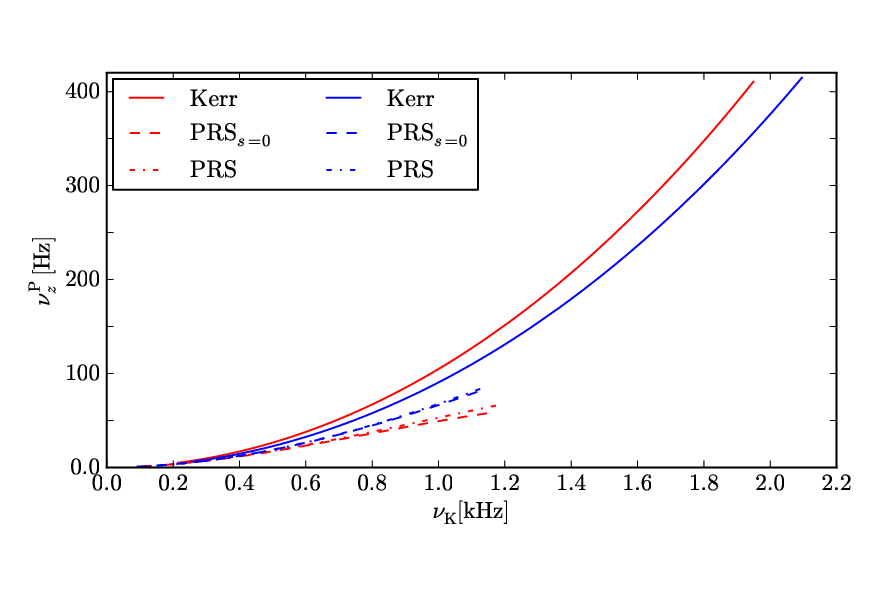
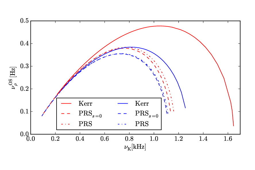
The deviations of the quadrupole and current octupole moments given by the Kerr solution from the numerical values of Pappas and Apostolatos (2012) can be used to show the low accuracy of the Kerr solution to describe fast rotating NSs. The accuracy of the PRS solution in describing the ISCO radii of these two models has been shown in Table 1 of Section III.
In Figs. 4 and 5 we can see the differences of the – and – relations between the Kerr and PRS solutions for realistic NS models. The deviations of the Kerr solution, especially at fast rotation rates, are evident because of the influence of the deformation (quadrupole ) of the star as well as, although in less proportion, of the octupole current . In general, we observe that the larger the angular momentum, the poorer the performance of the predictions of Kerr solution.
We have also shown in Figs. 4–5 the influence of the current octupole in the determination of the precession and oscillation frequencies. We found that the effect of is only appreciable for the fastest models. The minor influence, in this case, of the current octupole is expected from the small values of the parameter needed to fit the numerical values of Pappas and Apostolatos (2012). Clearly, larger values of the parameter needed to fit realistic values of will enhance as well deviations from the Kerr spacetime.
The effects of a multipolar structure that deviates from the one of the Kerr geometry on the various quantities analyzed here are relevant for instance in the RPM of the QPOs observed in LMXBs (see e.g. Stella and Vietri (1998); Morsink and Stella (1999); Stella et al. (1999); Stella and Vietri (1999) and Section VI, for details).
III.3. Dragging of Inertial Frames
It is known that a prediction of general relativity is that a rotating object makes a zero angular momentum test particle to orbit around it, namely it drags the particle into the direction of its rotation angular velocity; such an effect is called dragging of inertial frames or Lense-Thirring effect. Consequently, oblique particle orbit planes with respect to the source equatorial plane will precess around the rotation axis of the object. In stationary axially symmetric spacetimes described by the metric (1) the frame dragging precession frequency is given by (Ryan 1995, see e.g.)
| (26) |
Many efforts have been done to test the predictions of general relativity around the Earth such as the analysis of the periastron precession of the orbits of the LAser GEOdynamics Satellites, LAGEOS and LAGEOS II, (Lucchesi and Peron 2010, see e.g.) and the relativistic precession of the gyroscopes on-board the Gravity Probe B satellite (see Everitt et al. 2011, for details). The latter experiment measured a frame dragging effect within an accuracy of 19% with respect to the prediction of general relativity.
The smallness of this effect around the Earth makes such measurements quite difficult and has represented a multi year challenge for Astronomy. The frame dragging precession increases with the increasing of the angular momentum of the rotating object and therefore a major hypothetical arena for the searching of more appreciable Lense-Thirring precession is the spacetime around compact objects such as BHs and NSs. The much stronger gravitational field of these objects with respect to the Earth one allow them to attain much faster angular rotation rates and so larger angular momentum.
Stella and Vietri (1998) showed how, in the weak field slow rotation regime, the vertical precession frequency (orbital plane precession frequency) can be divided into one contribution due to the Lense-Thirring precession and another one due to the deformation (non-zero quadrupole moment) of the rotating object, both of them comparable from the quantitative point of view. These frequencies could be in principle related to the motion of the matter in the accretion disks around BHs and NSs and thus particularly applicable to LMXBs. For fast rotating NSs and BHs the frequency at which the orbital plane, and so the frame dragging precession frequency, can reach values of the order of tens of Hz (see e.g. Stella and Vietri (1998) and Figs. 3 and 4).
Thus, it is clear that an observational confirmation of the relativistic precession of matter around either a NS or a BH will lead to an outstanding test of the general relativity in the strong field regime and, at the same time, an indirect check of the large effects of the frame dragging in the exterior spacetime of compact objects (see e.g. Morsink and Stella 1999, for details).
Although making independent measurements of the frame dragging effect around BHs and NSs is a very complicate task, it is important to know the numerical values of the precession frequency due to the frame dragging with respect to other relativistic precession effects, e.g. geodetic precession. In addition, it is important to know the sensitivity of the precession frequency to the object parameters such as mass, angular momentum, quadrupole, and octupole moment.
In the upper panel of Fig. 6 we plotted contours of constant frame dragging frequency for the PRS solution, at the ISCO radius, as a function of the the angular momentum per unit mass and the quadruple moment , for a compact object mass . Correspondingly, in the lower panel of Fig. 6, we show the differences between the frame dragging precession frequency as predicted by the Kerr and PRS solutions, at the ISCO radius, as a function of and the difference between the quadrupole moments, .


The influence of the quadrupole moment in the determination of the frame dragging frequency is evident; the frequency given by a NS is generally smaller than the one given by a BH as can be seen from the value of the ratio obtained for configurations with a quadrupole moment that deviates with respect to the one given by the Kerr solution, namely for , see Eq. (11).
It is also worth mentioning that frame dragging precession can be affected as well by the presence of electromagnetic fields (Herrera et al. 2006, see) and further research in this respect deserves the due attention.
IV. Accuracy of Ryan’s Analytic Formulas
Following a series expansion procedure in powers of , Ryan (1995) found that the periastron (radial) and nodal (vertical) precession frequencies, and given by Eq. (24), can be written as a function of the Keplerian frequency as
| (27) |
and
| (28) |
where , are the lowest three mass moments and, , are the lowest two current moments. For the PRS solution in the vacuum case, .
The above formulas are approximate expressions of the periastron and nodal precession frequencies in the weak field (large distances from the source) and slow rotation regimes. We should therefore expect that they become less accurate at distances close to the central object, e.g. at the ISCO radius, and for fast rotating objects. However, such formulas are an important tool to understand the role of the lowest multipole moments on the values of the relativistic precession frequencies, such as the importance of the higher multipole moments at short distances and high frequencies as can be seen from Eqs. (27–28).
At high frequencies, for instance of the order of kHz, deviations from the above scaling laws are appreciable. In Figs. 7 and 8 we compare the radial precession and vertical oscillation frequencies, and , as a function of the Keplerian frequency , as given by the full expressions (24) for the PRS solution and by the approximate formulas (27) and (28), respectively.33 3 Because the scale of the and frequencies are very similar, we decided to plot in Fig. 7 and whose scales are different allowing a more clear comparison with the PRS solution in a single figure. The lowest multipole moments , , , and of the PRS solution have been fixed to the values of two models of the Table VI of Pappas and Apostolatos (2012); Model 2 with km (), , km3 ( g cm2), km4 and Model 20 with km (), , km3 ( g cm2) and km4.


In the – relation, the blue dotted curve depicts the contribution from the angular momentum (we plot the series (28) up to ), for the blue dot-dashed curve we added the first contribution from the quadrupole moment (we cut the series at ), for the dashed blue line we added the first contribution from the octupole mass-current (series expansion up to ) and finally in the continuos blue line we consider contributions for higher multipole moments and stop the series at the order , not shown in Eqs. (28). For this case, we can see that Ryan’s expressions clearly tend, from the bottom, to the exact result (continuous black curve) obtained by using the PRS solution.
For the analysis of the – relation we followed the same procedure as described above. In this case, the Ryan’s expressions tend from the top to the exact result, the continuous black curve, represented by the PRS solution. It is interesting to see that the introduction of the octupole moment (dashed red line) makes the approximation to deviate from the exact result, however by including more terms the accuracy is enhanced. As can be seen from Figs. 7 and 8 the quantitative accuracy of the Ryan’s approximate formulas in the periastron precession frequency is less than the one obtained in the vertical oscillation frequency .
The importance of the high-order multipole moments such as the quadrupole and the octupole moments is evident in the high-frequency regime. This is in line with the results shown in Figs. 2–3 and in Figs. 4–5. We can see from Figs. 7 and 8 that the Ryan’s approximate formulas describe more accurately the Model 2 than the Model 20. The reason is that, as we mentioned above, we should expect a better accuracy of the series expansions from low to moderate moderate rotation rates and consequently the same occur for the quadrupole deformations. It is clear that there are appreciable differences both in rotation and deformation between the two selected models; we recall also that the rotation frequency of the star can be expressed as a function of the dimensionless parameter as kHz.
It is noteworthy that we have checked that the Ryan’s series expansions, Eqs. (27) and (28), fit quite accurately the exact results if taken up to order . In particular the values of the vertical oscillation and precession frequencies are fit better than the corresponding radial ones. For the Model 2 the radial oscillation frequency is well fitted by the Ryan’s expression up to Keplerian frequencies of order kHz while, for the Model 20, the approximate formulas break down at a lower value kHz. These results are of particular relevance because it makes possible the extraction of the object parameters (for instance the lowest multipoles up to ) by the fitting of the observed QPO frequencies in LMXBs, providing they are indeed related to the precession and oscillation frequencies of matter in the accretion disk (see Section VI, for details) and for Keplerian motion not exceeding a few kHz of frequency.
V. Accuracy of PRS solution
We turn now to analyze the behavior of the Kerr and PRS solutions in predicting results for the Keplerian, frame dragging, and vertical oscillation frequencies, for realistic NSs. In particular, we compare their predictions with the frequencies calculated by Morsink and Stella (1999). Since Morsink and Stella (1999) did not include the values of the octupole current moment , here we set in Eq. (10) for the PRS solution. For the sake of comparison, we choose the results derived by Morsink and Stella (1999) for the EoS L, because for this EoS the highest rotating parameter and quadrupole moment were found. In addition, the stiffness of such an EoS allows the maximum mass of the NS to be larger than the highest observed NS mass, , corresponding to the 317 Hz (3.15 milliseconds rotation period) pulsar J1614-2230 (see Demorest et al. 2010, for details).
This regime of high and in realistic models is particularly interesting to test the deviations of the Kerr solution in the description of NS signatures as well as to explore the accuracy of the PRS solution. In Table 2, we present the results for four different sets of the star spin frequency , namely Hz (M1 and M2), Hz (M3 and M4), Hz (M5 and M6) and Hz (M7 and M8).
| Model | [km] | [kHz] | [Hz] | [Hz] | |||||||||||
|---|---|---|---|---|---|---|---|---|---|---|---|---|---|---|---|
| M1 | 1.88 | 0.19 | -5.3 | 15.4 | 14.90 | 15.42 | 1.31 | 1.363 | 1.304 | 39.7 | 42.248 | 38.476 | 18.6 | 39.697 | 22.040 |
| M2 | 2.71 | 0.14 | -3.0 | 22.2 | 22.16 | 22.23 | 0.90 | 0.906 | 0.902 | 19.6 | 19.676 | 19.493 | 17.2 | 18.809 | 17.629 |
| M3 | 1.94 | 0.24 | -8.2 | 15.6 | 14.89 | 15.63 | 1.29 | 1.380 | 1.296 | 49.8 | 57.001 | 49.804 | 17.5 | 52.608 | 26.197 |
| M4 | 2.71 | 0.18 | -4.8 | 21.8 | 21.62 | 21.74 | 0.93 | 0.937 | 0.931 | 26.1 | 27.245 | 26.833 | 21.9 | 25.670 | 23.635 |
| M5 | 2.07 | 0.40 | -23.1 | 16.3 | 14.18 | 16.06 | 1.26 | 1.514 | 1.289 | 84.3 | 125.75 | 88.905 | -10.5 | 109.04 | 31.140 |
| M6 | 2.72 | 0.30 | -13.9 | 20.6 | 20.05 | 20.45 | 1.01 | 1.041 | 1.015 | 53.5 | 57.467 | 54.391 | 35.8 | 51.861 | 42.854 |
| M7 | 2.17 | 0.51 | -39.4 | 17.0 | 13.58 | 16.53 | 1.22 | 1.637 | 1.269 | 106.7 | 201.52 | 116.25 | -51.8 | 166.55 | 29.804 |
| M8 | 2.73 | 0.39 | -24.4 | 19.8 | 18.85 | 19.65 | 1.06 | 1.136 | 1.077 | 78.8 | 90.821 | 80.895 | 38.4 | 79.079 | 57.187 |
In Table 2, we clearly observe that the results predicted by the PRSs=0 solution for the Keplerian and frame-dragging frequencies are in excellent agreement with those calculated by Morsink and Stella (1999) for even highly massive, rotating and deformed models such as the model M7 with , and . We notice that Morsink and Stella (1999) reported some configurations with negative values of (see Table 2). We advance the possibility that this is due to instabilities of the numerical code that occur when the ISCO radius is located very close or inside the surface of the object. Thus, the values of the frequencies given by the analytic solution in these cases are to be considered predictions to be tested for future numerical computations. This fact can be checked within the calculations of Morsink and Stella (1999) by exploring the properties of counter-rotating orbits which produce in general ISCO radii larger than the ones of the corotating ones. In Table 3, we depicted the results in the counter-rotating case where we can notice an improvement of the accuracy of the PRS solution with respect to the co-rotating case.
| Model | [km] | [kHz] | [Hz] | [Hz] | ||||||||
|---|---|---|---|---|---|---|---|---|---|---|---|---|
| M1 | 18.8 | 18.35 | 18.73 | 0.99 | 1.023 | 0.997 | 21.7 | 22.61 | 21.39 | 29.0 | 23.88 | 29.70 |
| M2 | 25.9 | 25.82 | 25.88 | 0.73 | 0.734 | 0.732 | 12.4 | 12.43 | 12.36 | 13.6 | 12.95 | 13.46 |
| M3 | 19.9 | 19.39 | 19.89 | 0.93 | 0.960 | 0.928 | 24.0 | 25.79 | 24.04 | 32.9 | 27.61 | 34.20 |
| M4 | 26.4 | 26.33 | 26.42 | 0.71 | 0.715 | 0.712 | 14.7 | 15.08 | 14.94 | 16.4 | 15.88 | 16.57 |
| M5 | 23.3 | 22.22 | 23.24 | 0.77 | 0.816 | 0.768 | 28.2 | 32.59 | 28.78 | 41.3 | 36.31 | 44.65 |
| M6 | 28.2 | 27.94 | 28.18 | 0.65 | 0.660 | 0.652 | 20.5 | 21.19 | 20.70 | 24.1 | 23.03 | 24.51 |
| M7 | 25.9 | 24.37 | 25.78 | 0.67 | 0.731 | 0.678 | 28.9 | 34.62 | 29.64 | 43.4 | 39.56 | 47.90 |
| M8 | 29.7 | 29.18 | 29.58 | 0.61 | 0.623 | 0.611 | 23.2 | 24.40 | 23.48 | 28.4 | 27.12 | 29.22 |
In this line, we consider worth performing numerical computations of the precession and oscillation frequencies of particles around realistic NSs in a wider space of parameters and using up-to-date numerical techniques which will certainly help to establish and elucidate more clearly the accuracy of analytic models. It is also appropriate recalling the recent results of Pappas and Apostolatos (2012) on the computation of the general relativistic multipole moments in axially symmetric spacetimes.
VI. The Relativistic Precision Model
The X-ray light curves of LMXBs show a variability from which a wide variety of QPOs have been measured, expanding from relatively low Hz frequencies all the way up to high kHz frequencies (see e.g. van der Klis 1995, for details). In particular, such frequencies usually come in pairs (often called twin peaks), the lower and upper frequencies, and respectively. BHs and NSs with similar masses can show similar signatures and therefore the identification of the compact object in a LMXB is not a simple task. If the QPO phenomena observed in these systems are indeed due to relativistic motion of accretion disk matter, the knowledge of the specific behavior of the particle frequencies (e.g. rotation, oscillation, precession) in the exterior geometry of NSs and BHs becomes essential as a tool for the identification of the nature of the compact object harbored by a LMXB.
It is not the scope of this work to test a particular model for the QPO phenomenon in LMXBs but instead to show the influence of the high multipole moments on the orbital motion of test particles especially the role of the quadrupole moment which is of particular interest to differentiate a NS from a BH. There are in the literature several models that describe the QPOs in LMXBs through the frequencies of particles around the compact object, and for a recent review and comparison of the different models we refer to the recent work of Lin et al. (2011). In order to show here the main features and differences between the Kerr and the PRS solutions we shall use the Relativistic Precession Model (RPM).
The RPM model identifies the lower and higher (often called twin-peaks) kHz QPO frequencies, and , with the periastron precession and Keplerian frequencies, namely and , respectively. The so-called horizontal branch oscillations (HBOs), which belong to the low frequency QPOs observed in high luminosity Z-sources (see e.g. van der Klis 1995, for details), are related within the RPM model to the nodal precession frequency of the same orbits (Morsink and Stella 1999, see). We will use here in particular the realistic NS models of Morsink and Stella (1999) for the EoS L.
One of the salient features of the RPM model is that in the case of the HBO frequencies, the relations inferred from the first term of the expansions (27) and (28)
| (29) | |||||
| (30) |
which implies a nodal precession frequency proportional to the square of the Keplerian frequency has been observed in some sources, for instance in the LMXB 4U 1728–34 (see Ford and van der Klis 1998, for details). In addition, power law relating the nodal and periastron precession frequencies can explain (Stella et al. 1999, see) the correlation between two of the observed QPO frequencies found in the fluxes of NSs and BHs LMXBs (see Psaltis et al. 1999, for details). This fact provides, at the same time, a significant test of the Ryan’s analytic expressions.
It is interesting to analyze the level of predictability of the precession and oscillation frequencies on particular astrophysical sources. In Fig. 9 we show the – relation within the RPM model, namely versus for the models M1–M8 of Table 2. In the upper panel we show the results for the PRS solution while, in the lower panel, we present the results for the Kerr solution. We have indicated the QPO frequencies observed in the sources GX 5–1 (Wijnands et al. 1998; Jonker et al. 2002, see e.g.), 4U 1735–44 (Ford et al. 1998, see e.g.), 4U 1636–53 (Wijnands et al. 1997, see e.g.), Sco X1 (van der Klis et al. 1996, see e.g.), GX 17–2 (Homan et al. 2002, see e.g.), GX 340+0 (Jonker et al. 2000, see e.g.), Cir X1 (van der Klis et al. 1996, see e.g.), 4U 0614+091 (Ford et al. 1997, see e.g.), and 4U 1728–34 (Strohmayer et al. 1996, see e.g.).


Both the upper and lower panels of Fig. 9 have been plotted using the same frequency scales in order to aid the identification of the differences between the Kerr and the PRS solutions. One can notice that all the solid curves in the Kerr solution (lower panel of Fig. 9) are outside the range of the observed QPO frequencies exemplified, while all dashed and solid curves of the PRS are inside the QPO range. It is then clear that making a fit of the observed QPO frequencies of the selected LMXBs of Fig. 9 will necessarily require a different choice of parameters in the Kerr and PRS solutions. Therefore, conclusions for instance on the NS parameters (e.g. mass, angular momentum, quadrupole deformation) based on fitting QPOs using the Kerr geometry will deviate from the actual parameters (see e.g. Laarakkers and Poisson 1999, for details), extractable more reliably from a more complex geometry, such as the PRS one, that allows a better estimate for instance of the quadrupole moment of a compact star.
In Fig. 9 we show the relation versus for the models M1–M8 of Table 2. For the sake of comparison we show the low frequency branch observed in the LMXB 4U 1728–34 (see Ford and van der Klis 1998, for details). From the analysis of the pulsating X-ray flux it turns out that very likely the spin frequency of the NS in 4U 1728–34 is Hz (see Strohmayer et al. 1996, for details). Thus, the models M3 (, ) and M4 (, ) in Table 2 that correspond to a NS of spin frequency Hz are of particular interest for the analysis of this source. It was suggested by Stella et al. (1999); Stella and Vietri (1999) that the low frequency observed in 4U 1728–34 are likely to be due to excitations of the second harmonic of the vertical motion and therefore a better fit of the lower-higher QPO frequencies of 4U 1728–34 (and of similar sources) will be obtained for the relation -. The black curves in Fig. 10 indicate the - relation for the models M3 and M4 (solid and dashed) following the above suggestion. Although the improvement of the fit is evident, we notice that the NS parameters that correctly reproduce the features of 4U 1728–34 are likely in between the models M3 and M4.


VII. Concluding Remarks
We have done an extensive comparison of the orbital motion of neutral test particles in the PRS and Kerr spacetime geometries. In particular we have emphasized on the Keplerian and frame-dragging frequencies, as well as the precession and oscillation frequencies of the radial and vertical motions.
We have evidentiated the differences in this respect between the Kerr and PRS solution, especially in the rapid kHz rotation regime. Such differences are the manifestation of the influence of the high order multipole moments such as the quadrupole and octupole.
The analysis of the deviations between the Kerr and PRS features for given mass and angular momentum of a source studied in this work are useful to distinguish the signatures between BHs and NSs, which relevant to establish a separatrix for the identification of the compact objects harbored in X-Ray Binaries. In the case of BH candidates, these results might become important for testing the no-hair theorem of BHs (Johannsen and Psaltis 2011, see e.g.). Equally important, the application of the precession and oscillation frequencies to the explanation of QPOs in LMXBs possessing a NS, can unveil information on the NS parameters, leading to a possible identification of the behavior of the nuclear matter EoS at supranuclear densities. In this line, the identification of the rotation frequency of NSs in LMXBs from the pulsating X-ray flux , e.g. the case of 4U 1728–34 (Ford and van der Klis 1998), 4U 1916–053 (Galloway et al. 2001) and more recently the case of IGR J17191–2821 (Altamirano et al. 2010), will certainly help to constrain QPO models as well as the NS parameters. Additional information coming from the photospheric radius expansion phenomena observed in these systems (see e.g. Muno et al. 2001, for details) during their transient activity with Super-Eddington emission can become of paramount importance if combined with the QPO information.
The generalization of the present work to the electrovacuum case is important to establish the influence of the magnetic dipole and quadrupole moments on the orbital motion of particles around compact objects (Bakala et al. 2010; Sanabria-Gómez et al. 2010; Bakala et al. 2012, see e.g.).
Interesting effects on the epicyclic frequencies due to the presence of the magnetic dipole have been already pointed out recently by Bakala et al. (2010) and Bakala et al. (2012). These effects were predicted after neglecting the contribution of the electromagnetic field to the curvature, for see Bakala et al. (2010) and for Bakala et al. (2012). Bakala et al. (2010) assumed the model of the star as a dipole magnetic field superposed on a Schwarzschild black hole. In the second work, they studied the case of a magnetized slowly rotating neutron stars; to build the model they superpose an dipolar magnetic field on the Lense-Thirring geometry. The effects of the magnetic dipole on the location of the ISCO, within the PRS solution, has been investigated by Sanabria-Gómez et al. (2010).
A complete analysis of the effects due to the emergence of electromagnetic structure on the orbital motion of charged particles is therefore of interest and deserve the appropriate attention. Recent observations have shown that for stars with strong magnetic fields the quadrupole and octupole magnetic terms make significant contributions to the magnetic field (Donati et al. 2006), which indicates that arbitrary higher order multipole components might be required in a realistic model. The presence of a magnetic quadrupole demands the breaking of the reflection symmetry (see Pachón and Sanabria-Gómez 2006, for details), by means of a slightly change to the Ernst electric potential over the symmetry axis
| (31) | ||||
a quadrupolar magnetic component can be introduced to the PRS solution. Such a change generates just a redefinition of the coefficients in Eq. (15). In this way the PRS solution can be readily use to explore the effect of strong magnetic fields with non-dipolar structure.
References
- Pachón and Sanabria-Gómez (2006) L. A. Pachón and J. D. Sanabria-Gómez, Classical and Quantum Gravity 23, 3251 (2006), arXiv:gr-qc/0603081 .
- Kerr (1963) R. P. Kerr, Physical Review Letters 11, 237 (1963).
- Laarakkers and Poisson (1999) W. G. Laarakkers and E. Poisson, Astrophys. J. 512, 282 (1999).
- Manko et al. (1995) V. S. Manko, J. Martín, and E. Ruiz, Journal of Mathematical Physics 36, 3063 (1995).
- Manko et al. (2000) V. S. Manko, J. D. Sanabria-Gómez, and O. V. Manko, Phys. Rev. D 62, 044048 (2000).
- Stephani et al. (2003) H. Stephani, D. Kramer, M. MacCallum, C. Hoenselaers, and E. Herlt, Exact solutions of Einstein’s field equations, 2nd ed. by Hans Stephani, Dietrich Kramer, Malcolm MacCallum, Cornelius Hoenselaers, and Eduard Herlt. Cambridge monographs on mathematical physics. Cambridge, UK: Cambridge University Press, 2003, edited by Stephani, H., Kramer, D., MacCallum, M., Hoenselaers, C., & Herlt, E. (2003).
- Stute and Camenzind (2002) M. Stute and M. Camenzind, Mon. Not. Roy. Astr. Soc. 336, 831 (2002), arXiv:astro-ph/0301466 .
- Berti and Stergioulas (2004) E. Berti and N. Stergioulas, Mon. Not. Roy. Astr. Soc. 350, 1416 (2004), arXiv:gr-qc/0310061 .
- Pachón et al. (2006) L. A. Pachón, J. A. Rueda, and J. D. Sanabria-Gómez, Phys. Rev. D 73, 104038 (2006), arXiv:gr-qc/0606060 .
- Sibgatullin and Sunyaev (1998) N. R. Sibgatullin and R. A. Sunyaev, Astronomy Letters 24, 774 (1998), arXiv:astro-ph/9811028 .
- Cook et al. (1994) G. B. Cook, S. L. Shapiro, and S. A. Teukolsky, Astrophys. J. 424, 823 (1994).
- Tomimatsu and Sato (1972) A. Tomimatsu and H. Sato, Physical Review Letters 29, 1344 (1972).
- Dubeibe et al. (2007) F. L. Dubeibe, L. A. Pachón, and J. D. Sanabria-Gómez, Phys. Rev. D 75, 023008 (2007), arXiv:gr-qc/0701065 .
- Stella and Vietri (1998) L. Stella and M. Vietri, Astrophys. J. Lett. 492, L59+ (1998), arXiv:astro-ph/9709085 .
- Morsink and Stella (1999) S. M. Morsink and L. Stella, Astrophys. J. 513, 827 (1999), arXiv:astro-ph/9808227 .
- Stella et al. (1999) L. Stella, M. Vietri, and S. M. Morsink, Astrophys. J. Lett. 524, L63 (1999), arXiv:astro-ph/9907346 .
- Stella and Vietri (1999) L. Stella and M. Vietri, Physical Review Letters 82, 17 (1999), arXiv:astro-ph/9812124 .
- Lin et al. (2011) Y.-F. Lin, M. Boutelier, D. Barret, and S.-N. Zhang, Astrophys. J. 726, 74 (2011), arXiv:1010.6198 [astro-ph.HE] .
- Johannsen and Psaltis (2011) T. Johannsen and D. Psaltis, Astrophys. J. 726, 11 (2011), arXiv:1010.1000 [astro-ph.HE] .
- Török et al. (2010) G. Török, P. Bakala, E. Šrámková, Z. Stuchlík, and M. Urbanec, Astrophys. J. 714, 748 (2010), arXiv:1008.0088 [astro-ph.HE] .
- Ryan (1995) F. D. Ryan, Phys. Rev. D 52, 5707 (1995).
- Papapetrou (1953) A. Papapetrou, Annalen der Physik 447, 309 (1953).
- Ernst (1968a) F. J. Ernst, Physical Review 167, 1175 (1968a).
- Ernst (1968b) F. J. Ernst, Physical Review 172, 1850 (1968b).
- Sibgatullin (1991) N. R. Sibgatullin, Oscillations and Waves in Strong Gravitational and Electromagnetic Fields, XIV, 362 pp. 26 figs.. Springer-Verlag Berlin Heidelberg New York. Also Texts and Monographs in Physics (1991).
- Manko and Sibgatullin (1993) V. S. Manko and N. R. Sibgatullin, Classical and Quantum Gravity 10, 1383 (1993).
- Hoenselaers and Perjes (1990) C. Hoenselaers and Z. Perjes, Classical and Quantum Gravity 7, 1819 (1990).
- Ruiz et al. (1995) E. Ruiz, V. S. Manko, and J. Martín, Phys. Rev. D 51, 4192 (1995).
- Bretón et al. (1999) N. Bretón, V. S. Manko, and J. Aguilar Sánchez, Classical and Quantum Gravity 16, 3725 (1999).
- Bakala et al. (2010) P. Bakala, E. Šrámková, Z. Stuchlík, and G. Török, Classical and Quantum Gravity 27, 045001 (2010).
- Sanabria-Gómez et al. (2010) J. D. Sanabria-Gómez, J. L. Hernández-Pastora, and F. L. Dubeibe, Phys. Rev. D 82, 124014 (2010), arXiv:1009.0320 [gr-qc] .
- Bakala et al. (2012) P. Bakala, M. Urbanec, E. Šrámková, Z. Stuchlík, and G. Török, Classical and Quantum Gravity 29, 065012 (2012).
- Pappas and Apostolatos (2012) G. Pappas and T. A. Apostolatos, (2012), arXiv:1201.6067v1 .
- Shibata and Sasaki (1998) M. Shibata and M. Sasaki, Phys. Rev. D 58, 104011 (1998).
- Lattimer and Prakash (2004) J. M. Lattimer and M. Prakash, Science 304, 536 (2004), arXiv:astro-ph/0405262 .
- Hessels et al. (2006) J. W. T. Hessels, S. M. Ransom, I. H. Stairs, P. C. C. Freire, V. M. Kaspi, and F. Camilo, Science 311, 1901 (2006), arXiv:astro-ph/0601337 .
- Herrera et al. (2006) L. Herrera, G. A. Gonzalez, L. A. Pachón, and J. A. Rueda, Classical and Quantum Gravity 23, 2395 (2006), arXiv:gr-qc/0602040 .
- Lucchesi and Peron (2010) D. M. Lucchesi and R. Peron, Physical Review Letters 105, 231103 (2010).
- Everitt et al. (2011) C. W. F. Everitt, D. B. Debra, B. W. Parkinson, J. P. Turneaure, J. W. Conklin, M. I. Heifetz, G. M. Keiser, A. S. Silbergleit, T. Holmes, J. Kolodziejczak, M. Al-Meshari, J. C. Mester, B. Muhlfelder, V. G. Solomonik, K. Stahl, P. W. Worden, Jr., W. Bencze, S. Buchman, B. Clarke, A. Al-Jadaan, H. Al-Jibreen, J. Li, J. A. Lipa, J. M. Lockhart, B. Al-Suwaidan, M. Taber, and S. Wang, Physical Review Letters 106, 221101 (2011), arXiv:1105.3456 [gr-qc] .
- Demorest et al. (2010) P. B. Demorest, T. Pennucci, S. M. Ransom, M. S. E. Roberts, and J. W. T. Hessels, Nature 467, 1081 (2010), arXiv:1010.5788 [astro-ph.HE] .
- van der Klis (1995) M. van der Klis, in IAU Colloq. 151: Flares and Flashes, Lecture Notes in Physics, Berlin Springer Verlag, Vol. 454, edited by J. Greiner, H. W. Duerbeck, and R. E. Gershberg (1995) p. 321.
- Ford and van der Klis (1998) E. C. Ford and M. van der Klis, Astrophys. J. Lett. 506, L39 (1998), arXiv:astro-ph/9808148 .
- Psaltis et al. (1999) D. Psaltis, T. Belloni, and M. van der Klis, Astrophys. J. 520, 262 (1999), arXiv:astro-ph/9902130 .
- Wijnands et al. (1998) R. Wijnands, M. Mendez, M. van der Klis, D. Psaltis, E. Kuulkers, and F. K. Lamb, Astrophys. J. Lett. 504, L35 (1998), arXiv:astro-ph/9806050 .
- Jonker et al. (2002) P. G. Jonker, M. van der Klis, J. Homan, M. Méndez, W. H. G. Lewin, R. Wijnands, and W. Zhang, Mon. Not. Roy. Astr. Soc. 333, 665 (2002), arXiv:astro-ph/0202420 .
- Ford et al. (1998) E. C. Ford, M. van der Klis, J. van Paradijs, M. Méndez, R. Wijnands, and P. Kaaret, Astrophys. J. Lett. 508, L155 (1998), arXiv:astro-ph/9809407 .
- Wijnands et al. (1997) R. A. D. Wijnands, M. van der Klis, J. van Paradijs, W. H. G. Lewin, F. K. Lamb, B. Vaughan, and E. Kuulkers, Astrophys. J. Lett. 479, L141 (1997).
- van der Klis et al. (1996) M. van der Klis, J. H. Swank, W. Zhang, K. Jahoda, E. H. Morgan, W. H. G. Lewin, B. Vaughan, and J. van Paradijs, Astrophys. J. Lett. 469, L1 (1996), arXiv:astro-ph/9607047 .
- Homan et al. (2002) J. Homan, M. van der Klis, P. G. Jonker, R. Wijnands, E. Kuulkers, M. Méndez, and W. H. G. Lewin, Astrophys. J. 568, 878 (2002), arXiv:astro-ph/0104323 .
- Jonker et al. (2000) P. G. Jonker, M. van der Klis, R. Wijnands, J. Homan, J. van Paradijs, M. Méndez, E. C. Ford, E. Kuulkers, and F. K. Lamb, Astrophys. J. 537, 374 (2000), arXiv:astro-ph/0002022 .
- Ford et al. (1997) E. C. Ford, P. Kaaret, K. Chen, M. Tavani, D. Barret, P. Bloser, J. Grindlay, B. A. Harmon, W. S. Paciesas, and S. N. Zhang, Astrophys. J. Lett. 486, L47 (1997), arXiv:astro-ph/9706100 .
- Strohmayer et al. (1996) T. E. Strohmayer, W. Zhang, J. H. Swank, A. Smale, L. Titarchuk, C. Day, and U. Lee, Astrophys. J. Lett. 469, L9 (1996).
- Galloway et al. (2001) D. K. Galloway, D. Chakrabarty, M. P. Muno, and P. Savov, Astrophys. J. Lett. 549, L85 (2001), arXiv:astro-ph/0010072 .
- Altamirano et al. (2010) D. Altamirano, A. Watts, M. Linares, C. B. Markwardt, T. Strohmayer, and A. Patruno, Mon. Not. Roy. Astr. Soc. 409, 1136 (2010), arXiv:1005.5299 [astro-ph.HE] .
- Muno et al. (2001) M. P. Muno, D. Chakrabarty, D. K. Galloway, and P. Savov, Astrophys. J. Lett. 553, L157 (2001), arXiv:astro-ph/0105042 .
- Donati et al. (2006) J.-F. Donati, I. D. Howarth, M. M. Jardine, P. Petit, C. Catala, J. D. Landstreet, J.-C. Bouret, E. Alecian, J. R. Barnes, T. Forveille, F. Paletou, and N. Manset, Mon. Not. Roy. Astr. Soc. 370, 629 (2006), arXiv:astro-ph/0606156 .
Appendix A Metric Functions
The functions , , , , , , and used to express the metric functions (17) are given by
| (A1) | ||||
| (A2) | ||||
| (A3) | ||||
| (A4) |
with
and
being ’s the roots of the Sibgatullin equation Sibgatullin (1991); Manko and Sibgatullin (1993)
| (A5) |
Appendix B Kerr’s metric in Weyl-Papapetrou quasi-cylindrical coordinates
In order to keep comparisons in the save place, we consider useful to display the Kerr solution in the Weyl-Papapetrou quasi-cylindrical coordinates. For this case,
| (B1) |
where for our own convenience we do not present the definition of each term, but present the final combination of them, i.e.,
| (B2) | ||||
| (B3) | ||||
| (B4) | ||||
| (B5) | ||||
From here, it is clear how changing will cause only a global change in the sign of the metric function and therefore only a change in the metric component.