Muon diffusion in diluted paramagnetic systems
Abstract
Muon Spin Rotation/Relaxation (SR) is a powerful probe to study diffusion of hydrogen-like particles. One of the most common model to analyze SR signals from materials where diffusion occurs, is by using functions derived from the stochastic theory of Kubo and Toyabe along with the strong collision model. Unfortunately the current formalism can not be used to analyze data from systems where not only muons diffuse, but also the magnetic moments of the material are dynamic. In this article we introduce a new model which accounts for both dynamical effects, and use this model to analyze SR signals from .
pacs
76.75.+i, 66.30.j-I Introduction
The study of muon diffusion is a topic of interest not only for science but also for technology, since the muon can be thought of as a light proton [1, 2]. Muon diffusion is measured using the Muon Spin Rotation/Relaxation (SR) technique. In this technique polarized muons are implanted in a sample, and the positrons arising from their asymmetric decay are recorded as a function of time and direction [3]. With this information one may reconstruct the time dependent polarization signal of the muon ensemble. The analysis of this signal provides important information about the local magnetic environment and, if present, about the muon diffusion rate.
The most common model used to analyze SR signals from systems where muons diffuse is based in the probabilistic theory of R. Kubo and T. Toyabe [4] together with the strong collision approximation [4, 5, 6]. In its simplest version this model assumes that, after the muons are implanted, they sense a local static field which is random and has a Gaussian distribution. For paramagnetic systems this local magnetic field is typically originated by the nuclear magnetic moments, which are static within the SR time window. The model assumes also that the muons can hop between minima of potential with a hopping rate , and therefore the muons see instantaneous field changes with this same rate. This model, which is referred as the Dynamical Gaussian Kubo-Toyabe (DGKT) model, is suited to analyze signals from materials where the magnetic moments are densely packed. For magnetically diluted systems though, the internal field distribution is not Gaussian but Lorentzian [7, 8].
No standard model exist to analyze signals if both, muon diffusion and fluctuations of the magnetic moments of the system, are present. As we will see in the next section, in magnetically dense systems a DGKT-like model cannot disentangle muon hopping rates from fluctuations of the magnetic moments of the system. Nevertheless, this is not the case for magnetically diluted materials, and we report here a model suited to analyze signals from this type of systems. Using numerical simulations of this model we have found that magnetically diluted systems are specially well suited to study muon diffusion, since its onset produces a change on the shape of the relaxing signal (even if the hopping rate is much smaller than the fluctuation rate of the magnetic moments). After this, in Section III we present a set of phenomenological formulas derived from our simulated polarization functions, and which can be used to analyze experimental data. In Section IV we use these formulas to analyze data from ; and then in section V, we discuss the results and comment on the limits of the model.
II A model for muon diffusion with magnetic moment fluctuations
In the Gaussian Kubo-Toyabe (GKT) model [9, 3] the local field at each muon site is taken randomly from a Gaussian field distribution:
| (1) |
where:
| (2) |
In this last equation is the muon gyromagnetic ratio (2 135.54MHz/T), is the width of the field distribution, and is one of the three components of the magnetic field. Since the local field at each muon site is static, then the polarization of the muon ensemble can be analytically calculated and is given by:
| (3) |
The GKT model describes systems of Heisenberg magnetic moments which fill completely the sites of the lattice and which are static. If the field sensed by the muons changes due to fluctuations of these magnetic moments, then the strong collision model can be used to model the effect of these fluctuations on the muon polarization. In this strong collision model [9, 3] the field change is a Markovian processes with a characteristic fluctuation rate (i.e. after a time the local field changes instantaneously to other taken randomly from the field distribution in Eq. 2). The resulting dynamical model is the DGKT one mentioned in the introduction. Now, if the local magnetic moments are static but the muons are diffusing at a rate (and assuming that the field at the new site where the muon hops is uncorrelated with the previous one), then the field sensed by the muons will be effectively fluctuating with a rate , and the strong collision model can be also applied to describe the muon diffusion process. Then, in the DGKT model fluctuations of the magnetic moments are completely equivalent to a muon diffusion process; therefore, in magnetically dense systems it is not possible to distinguish one dynamic process from the other. This is not the case for magnetically diluted systems as we will show in the following.
Lets assume a static scenario again, but now most of the magnetic moments have been removed (i.e. substituted) from the lattice. In this diluted system the muons which thermalize near to a magnetic moment can sense higher fields than those which land far from a magnetic moment. This means that many magnetically inequivalent muon sites are present in a diluted system. Mathematically, this can be model by introducing a distribution of . This distribution is given by [10]:
| (4) |
where is the characteristic width of the distribution. If the field distribution in Eq. 1 is averaged with the distribution on Eq. 4, the total magnetic field distribution seen by the muon ensemble is the three dimensional generalization of the Lorentzian distribution as required for a diluted magnetic system [7, 8]:
| (5) |
where is the magnitude of the local field. The static polarization signal which arises from this field distribution is:
| (6) |
If the field at the muon site changes due to fluctuations of the magnetic moments of the material, then the dynamical behavior is introduced with the strong collision model [9, 3]. Note though, that muons which land in an specific region of the material will sense fluctuating fields with a distribution characterized by a local ; and muons which land in other regions will sense fluctuating local fields with a different local . Mathematically this amounts to making the time average (applying the strong collision model) before the spatial average (average over with Eq. 4) [9, 6]. SR signals with this Fluctuating Lorentzian Kubo-Toyabe (FLKT) model are shown in the upper panel in Fig. 1 for different fluctuation rates (). We want to notice two things. One is the strong depolarizing effect of dynamic fields (the polarization of the muon ensemble goes to zero at long times, while it is equal to 1/3 in the static case); and second, the decrease in the relaxation rate of the polarization signal at high fluctuation rates. This last effect is known as the narrowing effect, and it happens because the local field is fluctuating so fast that the muons do not have time to precess much in the instantaneous local field. An important characteristic of the signal in the narrowing limit is its square-root exponential trend[9, 3]:
| (7) |

Now, we will assume that the magnetic moments are static but muons can hop from site to site. To account for this dynamical effect we have used the strong collision model again , but now we have performed the time average after the spatial average. This means that a single muon can probe the whole distribution in Eq. 5 as it hops through the lattice (assuming again that the field from site to site is uncorrelated), and not only one specific . Then, muons are able to sense a bigger range of fields as they diffuse faster and faster. The lower panel in Fig. 1 shows several muon polarization signals using this Hopping Lorentzian Kubo Toyabe (HLKT) model. Notice that no narrowing effect is observed. Further more, at high hopping rates the signal is exponential and independent of the hopping rate [11, 10]:
| (8) |
The absence of the narrowing effect in the HLKT model is a problem of the Lorentzian field distribution, which allows for the muon to sense unphysically large magnetic fields [11]. To appreciate this, we have calculated the probability that a muon senses a field bigger than when hoping into a new site (at these fields the muons will be able to make a big precession before hoping to an other site and therefor reduce the polarization of the ensemble). At high hoping rates () this probability is . This can be used to calculate the probability that within the signal time window (typically 10 s) the muon sense a highly depolarizing field. This probability is equal to ( is the signal time window) and it is independent of . This means that as is increased more and more the signal will tend to a independent relaxation rate. This unphysical behavior of the HLKT model could be avoided by introducing a maximum field cutoff in the distribution on Eq. 5. This cutoff is system dependent and should be calculated carefully. This type of refinement of the model is outside the scope of this document. Never the less, the HLKT model is valid as long as .
We have extended the Lorentzian Kubo-Toyabe formalism to account for systems where the magnetic moments fluctuate and also muons diffuse. In this model, which we will call the Extended Lorentzian Kubo-Toyabe (ELKT) model, the dynamical behavior is also introduced by the strong collision model, but this time before and after the spatial average to account for the magnetic moment fluctuations and muon hoping respectively. We have studied this model numerically using a Monte Carlo algorithm. At time zero, this algorithm selects a for the local field distribution with a probability given by Eq. 4. Then, the local field is allowed to to fluctuate with a fluctuation rate . The local field fluctuations are carried on until a muon-hop event happens, and this occurs with a frequency given by the muon hopping rate . At this point a new is randomly chosen from the probability distribution on Eq. 4 and, again, the local field is allowed to fluctuate with a field distribution characterized by the new field width. In between all these “collisions” the muon polarization function is properly evolved, and it is recorded into an array at a discrete set of times.
Since our interest is to study the effect of muon diffusion in fast fluctuating paramagnetic materials (see Section IV), we have performed all our simulations in the narrowing limit (). Fig. 2 shows the effect of increasing the muon hopping rate on the SR signal from a diluted paramagnetic system. The signal is a root exponential in the absence of muon diffusion and equal to Eq. 7. As the muon hopping rate is increased, the signal shape changes continuously to an exponential at high diffusion rates. In the high hopping rate limit the signal is given by Eq. 8.

III Phenomenological description of the ELKT model
In order to use the numerical solutions of the ELKT model to analyze experimental data (see next section), we have fitted our simulated signals in the narrowing limit () to a stretched exponential function:
| (9) |
Fig. 3 shows the dependence of and on the muon hopping rate. Note that, as the muon hopping rate is increased from zero, the parameter grows from 0.5 to 1 as expected. We have found that the dependence of and on the field fluctuating rate, muon hopping rate and is well described by (see Fig. 3):
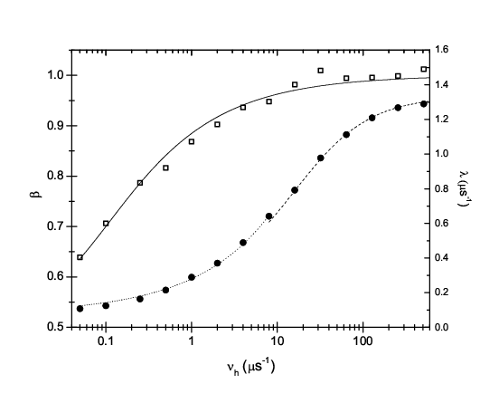
| (10) |
| (11) |
| (12) |
where and refer to different ranges where each equation apply. describes the dependence for , and for .
We want to mention that, as a log(log()) vs. log(t) plot shows, the numerical solutions of the ELKT model are close to stretched exponentials but are not equal. Nevertheless we have used this function because is commonly used in the analysis of SR signals and it will allows us to understand previous published works (see Section V). In the next section we use Eq. 10 and 11 to obtain quantitative measurements of the muon diffusion rate in .
IV Muon diffusion in
The low temperature behavior of the ionic insulator have had much attention from researchers [12]. Below 20K, the Dy3+ magnetic ions have an Ising character and they form a magnetically frustrated system due to their effectively antiferromagnetic interactions and to their arrangement in a lattice of corner shearing tetrahedra. Below 4K, the magnetic ions arrange such that two spins point inside every tetrahedra and two out. This arrangement of spins can be mapped into that of hydrogen atoms in watter ice, and therefore this ground state is often referred as spin ice. More recently, it was noticed that the spin ice state is a background for topological excitations which behave as magnetic monopoles [13, 14].
We have used SR to study the effect of magnetic dilution in this system by substituting magnetic Dy3+ ions with non magnetic Y3+. A single crystal of was grown using an optical floating zone furnace. The single crystal was aligned using a Laue camera and cut such that the muons are implanted with their spin parallel to the (110) direction. All the sample preparation was performed in the Laboratory for Developments and Methods in the Paul Scherrer Institut (PSI, Switzerland). The SR measurements were performed at the GPS instrument at PSI, and which is located in the M3 beam line. We performed temperature scans between 2K and 250K in an applied field of 100G transverse to the muon polarization. Also, we have performed complementary measurements with the field applied along the muon spin direction and in zero field.
Fig. 4 shows a SR signal from at 160K where the system is paramagnetic. Note in this picture the stretched exponential-like envelope of the signal. For this reason, we first fitted the data to a cosine function times a stretched exponential envelope. The left panel in Fig. 5 shows that the parameter increased with temperature from a value of 0.59 below 100K to 0.94 at 250K, and decreased monotonically from 21s-1 to 0.2s-1 in the same range. As we mentioned in the previous section, the ELKT model can explain the trend in in terms of an onset of muon diffusion upon warming. Nevertheless, and according to Fig. 3, an onset of muon diffusion would produce an increase of with temperature. This is in contrast with what we observe. As we will see later, the decrease of with temperature is also captured by the ELKT model, and it is due to the fact that the thermally activated fluctuations of the Dy magnetic moments are much bigger than the muon hopping rate (see Eq. 11). Then, we analyzed our data by fitting the relaxing envelop to a stretched exponential where the relaxation rate is given by Eq. 11 and the coefficient by a modified version of Eq. 10. This modification consist on substituting the 1/2 factor on the right hand side of Eq. 10 by 0.41, such that for T120K is equal to the experimentally observed value of 0.59 . This apparently ad hoc modification is justified by the fact that, even if the dilution is significant in our system, it is not in the very high dilution regime which the ELKT model assumes (20% of the DY/Y sites are occupied by magnetic ions in ). As shown by Noakes[7], as a system is magnetically diluted the relaxation function changes continuously from a Gaussian Kubo-Toyabe to a Lorentzian Kubo-Toyabe. This means that in the narrowing limit, the coefficient of the stretched exponential will change from 1 to 0.5 continuously as the system is magnetically diluted. Our system is concentrated enough, such that this coefficient is slightly above 0.5
It is well known that in the characteristic fluctuation rate of the magnetic moments in the paramagnetic state is thermally activated [15, 16], and therefor the fluctuation rate of the local field at the muon site will be given by[6]:

| (13) |
where is the energy gap between the ground state doublet and the first excited crystal field level. The reported values for this number ranges from 200K to 380K [15, 17]. In the absence of spectroscopic data, we used a value equal to 300K. In order to determine we used a longitudinal field measurement at 60K to determine the fluctuation rate of the local magnetic field at this temperature. Assuming that the muons do not diffuse at these temperature (this is indicated by a temperature independent of approximately 0.59), we have obtained a fluctuation rate of 990MHz at this temperature. Using this value in Eq. 13, we have obtained =150GHz, which is close to that found by neutron spin echo measurements (220GHz) [16]. Then, when we analyzed our data we set to the value given by Eq. 13 and extracted and from the fit at each temperature.
The fitted values for and are shown in the right panel in Fig. 5. Note the big error bars on for T80K. This only reflects the very steep grow of at low values of (see Eq. 10). Figure 5 shows that muons start to diffuse between 120K and 140K, and the diffusion rate grows until 200K and then stays constant. Below 80K, the parameter is constant and equal to 100s-1. This is close to 110s-1, value that we found at 2K where the system is almost static within our time window. As the temperature grows the value of decreases due to the different orientations that the magnetic moments can have in the higher crystal field level.

V Comments
As shown in the previous section, the ELKT model is able to explain the increase of with temperature in in terms of the onset of muon diffusion. This increase of with temperature has been observed in an other ionic insulator [18, 19], but no explanation of this effect was provided. Campbell et al. [20] observed an increase of with temperature in the canonical spin-glass AgMn at high temperature [21]. The authors mentioned that this effect could be produced by muon diffusion but no further analysis of the data was performed. This study also pointed out that the increase in was accompanied by an increase, and subsequent saturation, of the relaxation rate of the signal upon cooling. The authors interpreted this as a consequence of muon retraping near the magnetic impurities. In our case the relaxation rate of the signal decreases monotonically with temperature up to 250K. Nevertheless, the ELKT model shows a saturation of above 160K (see Fig. 5). It is not possible to know with the data taken if this saturation is due to muon retraping (the slightly different ionic radius of Y and Dy create local distortions in the lattice [22] which might favor some muon sites over others). Nevertheless, we want to note that if a muon retraping process is present in , then the ELKT model would provide only with an “averaged” muon diffusion rate since this model posses only one diffusion parameter (instead of the three dynamical parameters needed to describe diffusion with a single retraping mechanism[3]). Still, and even if muon retraping is present, the increase in from 0.59 to 0.94 remains a signature of the onset of muon diffusion since its change is produced by the muon exploring different regions of the material with different magnetic moment densities (i.e. different characteristic field widths ). This fact is confirmed by our low transverse field measurements in a sample of , where we found that the parameter is temperature independent and equal to 1 within error bars. This is expected by the theory since this sample is magnetically dense, and therefore all muon sites have approximately same local density of magnetic moments (i.e. the same field width ).
We want to finish this section by reviewing a couple of limitations of the ELKT model. One limitation is the spherical nature of the internal field distribution which the ELKT model assumes (see Eq. 1). Care should be taken when using Kubo-Toyabe models to fit single crystal data since the internal field distributions have not, in general, spherical symmetry. Nevertheless the biggest discrepancies are expected to be observed at low values of and not so much at the high fluctuation rates explored in this work [18]. An other limitation of the ELKT is that it assumes that the magnetic fluctuations are characterized by a single fluctuation rate of the local magnetic field (). Then, it should not be used to model magnetic systems with a richer dynamic response such as spin-glasses relatively close to .
VI Conclusions
We have introduced the ELKT model which is suited to analyze SR signals from diluted magnetic systems where muon diffusion is present and where the magnetic moments are dynamic. Also, we have provided a set of phenomenological formulas to extract muon diffusion rates from systems where the magnetic background fluctuates fast. We have used these formulas to analyze data from , and found that muons diffuse for T140K. Also, we have found that the diffusion rate saturates for T180K. We have shown that the increase with temperature of the parameter in a hot diluted paramagnet is produced by the onset of muon diffusion, and this is further confirmed by our observation that this parameter is temperature independent in a magnetically dense system. We believe that the use of the ELKT model can allow to study muon diffusion by introducing a small amount of strong magnetic impurities in a system where muon diffusion can not be studied otherwise (e.g. in systems with small nuclear magnetic moments).
References
- [1] V. G. Storchak and N. V. Prokof’ev, Rev. Mod. Phys. 70, 929 (1998).
- [2] G. Alefeld and J. Völkl, eds., Hydrogen in metals I, vol. 28 of Topics in applied physics (Springer-Verlag, 1978).
- [3] A. Yaouanc and P. D. de Réotier, Muon spin rotation, relaxation, and resonance: applications to condensed matter, vol. 147 of International Series of Monographs on Physics (Oxford Science Publications, 2011).
- [4] R. Kubo and T. Toyabe, in Magnetic resonance and relaxation : proceedings of the XIVth Colloque Ampère, Ljubljana, 6-11 September 1966, edited by R. Blinc (North Holand, Amsterdam, 1967), pp. 810–823.
- [5] R. S. Hayano, Y. J. Uemura, J. Imazato, N. Nishida, T. Yamazaki, and R. Kubo, Phys. Rev. B 20, 850 (1979).
- [6] Y. J. Uemura, T. Yamazaki, D. R. Harshman, M. Senba, and E. J. Ansaldo, Phys. Rev. B 31, 546 (1985).
- [7] D. R. Noakes, Phys. Rev. B 44, 5064 (1991).
- [8] R. E. Walstedt and L. R. Walker, Phys. Rev. B 9, 4857 (1974).
- [9] Y. J. Uemura, in Muon science: muons in physics, chemistry, and materials : proceedings of the fifty first Scottish Universities Summer School in Physics, St. Andrews, August 1998, edited by S. Lee, S. Kilcoyne, and R. Cywinski (Scottish Universities Summer School in Physics, 1999), Scottish universities summer school, pp. 85–114.
- [10] Y. J. Uemura, Hyperfine Interact. 8, 739 (1981).
- [11] A. Fiory, Hyperfine Interact. 8, 777 (1981).
- [12] M. Gingras, in Introduction to frustrated magnetism: materials, experiments, theory, edited by C. Lacroix, P. Mendels, and F. Mila (Springer Heidelberg Dordrecht London New York, 2011), Springer series in solid-state sciences, pp. 293–325.
- [13] C. Castelnovo, R. Moessner, and S. L. Sondhi, Nature 451, 42 (2008).
- [14] L. D. C. Jaubert and P. C. W. Holdsworth, Nat. Phys. 5, 258 (2009).
- [15] J. Snyder, J. Slusky, R. Cava, and P. Schiffer, Nature 413, 48 (2001).
- [16] G. Ehlers, A. Cornelius, M. Orendac, M. Kajnakova, T. Fennell, S. Bramwell, and J. Gardner, J. Phys.: Condens. Matter 15, L9 (2003).
- [17] S. Rosenkranz, A. Ramirez, A. Hayashi, R. Cava, R. Siddharthan, and B. Shastry, J. Appl. Phys. 87, 5914 (2000).
- [18] J. Rodriguez, Ph.D. thesis, McMaster University (2009).
- [19] R. C. Johnson, K. H. Chen, S. R. Giblin, J. S. Lord, A. Amato, C. Baines, B. Barbara, B. Z. Malkin, and M. J. Graf, Phys. Rev. B 83, 174440 (2011).
- [20] I. A. Campbell, A. Amato, F. N. Gygax, D. Herlach, A. Schenck, R. Cywinski, and S. H. Kilcoyne, Phys. Rev. Lett. 72, 1291 (1994).
- [21] The increase in explained in this document should not be confused with that observed in spin-glasses as one warms up from . This last one is produced by a broadening of the dynamic response of the system at low temperature, while that presented in this document is due to muon diffusion.
- [22] J. Snyder, B. G. Ueland, A. Mizel, J. S. Slusky, H. Karunadasa, R. J. Cava, and P. Schiffer, Phys. Rev. B 70, 184431 (2004).